Sustained Magnetorotational Turbulence in Local Simulations of Stratified Disks with Zero Net Magnetic Flux

Abstract

We examine the effects of density stratification on magnetohydrodynamic turbulence driven by the magnetorotational instability in local simulations that adopt the shearing box approximation. Our primary result is that, even in the absence of explicit dissipation, the addition of vertical gravity leads to convergence in the turbulent energy densities and stresses as the resolution increases, contrary to results for zero net flux, unstratified boxes. The ratio of total stress to midplane pressure has a mean of $\sim 0.01$, although there can be significant fluctuations on long ($\gtrsim 50$ orbit) timescales. We find that the time averaged stresses are largely insensitive to both the radial or vertical aspect ratio of our simulation domain. For simulations with explicit dissipation, we find that stratification extends the range of Reynolds and magnetic Prandtl numbers for which turbulence is sustained. Confirming the results of previous studies, we find oscillations in the large scale toroidal field with periods of $\sim 10$ orbits and describe the dynamo process that underlies these cycles.

1. Introduction

The magnetorotational instability (MRI) plays an important role in determining the angular momentum transport rate (and therefore accretion rate) in most astrophysical disks (Balbus & Hawley, 1998). Therefore it is of considerable interest to understand what determines the saturation amplitude of the MRI in the nonlinear regime. Investigations of this question generally utilize numerical methods to study the time-dependent MHD in the local, shearing box approximation.

From the first three-dimensional studies (Hawley et al., 1995), it has been known that for uniform density the saturation amplitude depends on parameters such as the net flux and geometry of the magnetic field threading the domain (Sano et al., 2004). More recently, there has been considerable interest in the effect of microscopic dissipation, such as Ohmic resistivity and Navier-Stokes viscosity, on the saturation amplitude with various initial field geometries (Fromang et al., 2007; Lesur & Longaretti, 2007; Simon & Hawley, 2009), as well as the effect of the radial extent of the domain (Bodo et al., 2008; Johansen et al., 2009; Guan et al., 2009).

One particularly important and puzzling result is that in the special case of no net magnetic flux with no explicit dissipation, the saturation amplitude of the MRI decreases with increasing resolution (Fromang & Papaloizou, 2007; Pessah et al., 2007). In this case, it appears the amplitude of the microscopic diffusivities determines the saturation amplitude of the MRI. Although this result is of considerable interest from a theoretical perspective in understanding the MRI and MHD turbulence, it is not yet obvious it has application to real disks, in which the magnetic flux is unlikely to be zero in every local patch for all time (Sorathia et al. 2009), and which are vertically stratified.

Although the saturation of the MRI has been studied in the local shearing box approximation in vertically stratified disks (Brandenburg et al., 1995; Stone et al., 1996), these early studies lacked sufficient computational resources to perform a systematic convergence study, or evolve the disk for hundreds of orbital times in order to measure accurately the saturation amplitude. In this paper, we use modern numerical methods to revisit the saturation of the MRI in vertically stratified disks with no initial net magnetic flux. Interestingly, in this case we find quite different results compared to the unstratified boxes studied by Fromang & Papaloizou (2007). In the stratified boxes studied here, the stress converges with numerical resolution even with no explicit dissipation, In fact, with explicit dissipation, we find in stratified disks there can be significant and sustained turbulence at magnetic Reynolds numbers that suppress the turbulence in unstratifed disks (Fromang et al., 2007). These results seem to be a consequence of an MHD dynamo that operates in stratified disks, and we explore the properties of this dynamo in this paper.

This paper is organized as follows. In §2 we summarize the most relevant properties of our numerical methods and describe our Fourier analysis. In §3 we report our results: the outcome of our resolution study in §3.1; the dependence on the vertical and radial aspect ratios in §3.2 and §3.3; and the effects of adding finite dissipation in §3.4. In §4 we discuss the nature of the dynamo driving the sustained turbulence, and in §5 we summarize our conclusions.

2. Method

We use Athena (Gardiner & Stone, 2005, 2008; Stone et al., 2008) for all calculations presented in this work. We perform 3d MHD simulations, adopting the local shearing box formalism and including vertical gravity. We refer the reader to Stone & Gardiner (2009) for a detailed discussion of the equations, algorithms, and boundary conditions specific to the shearing box, as well as a description of their implementation in Athena. Here we just summarize the basic equations and the most relevant features for our current work.

The local shearing box approximation adopts a frame of reference located at a fiducial radius corotating with the disk at orbital frequency $\Omega$. In this frame, the equations of ideal MHD are written in a Cartesian coordinate system $(x,y,z)$ that has unit vectors $({\hat{\mbox{\boldmath{$i$}}}},{\hat{\mbox{\boldmath{$j$}}}},{\hat{\mbox{\boldmath{$k$}}}})$ as

$$\frac{\partial\rho}{\partial t}+{\mbox{\boldmath{$\nabla$}}\cdot}[\rho{\mbox{\boldmath{$v$}}}] = 0,$$ (1)

$$\frac{\partial\rho{\mbox{\boldmath{$v$}}}}{\partial t}+{\mbox{\boldmath{$\nabla$}}\cdot}\left[\rho{\mbox{\boldmath{$v$}}v}+{\sf T}\right] = \rho\Omega^{2}(2qx{\hat{\mbox{\boldmath{$i$}}}}-z{\hat{\mbox{\boldmath{$k$}}}})-2\Omega{\hat{\mbox{\boldmath{$k$}}}}\times\rho{\mbox{\boldmath{$v$}}},$$ (2)

$$\frac{\partial{\mbox{\boldmath{$B$}}}}{\partial t}-{\mbox{\boldmath{$\nabla$}}}\times\left({\mbox{\boldmath{$v$}}}\times{\mbox{\boldmath{$B$}}}\right) = 0,$$ (3)

where ${\sf T}$ is the total stress tensor

$${\sf T}=(p+B^{2}/2){\sf I}-{\mbox{\boldmath{$B$}}^{\rm T}}{\mbox{\boldmath{$B$}}},$$ (4)

${\sf I}$ is the identity matrix, $\rho$ is the gas density, $p$ is the gas pressure, $B$ is the magnetic field, $v$ is the velocity and $B^{2}={\mbox{\boldmath{$B$}}}\cdot{\mbox{\boldmath{$B$}}}$. The shear parameter $q$ is defined as

$$q=-\frac{d{\rm ln}\Omega}{d{\rm ln}r}$$ (5)

so that for Keplerian flow $q=3/2$. We adopt an isothermal equation of state with $p=c_{\rm s}^{2}\rho$.

In §3.4 we also present simulations which include terms for constant scalar viscosity and resistivity. The viscous term is ${\mbox{\boldmath{$\nabla$}}\cdot}{\sf M}$ with

$${\sf M}_{ij}=\rho\nu\left(\frac{\partial v_{i}}{\partial x_{j}}+\frac{\partial v_{j}}{\partial x_{i}}-\frac{2}{3}\delta_{ij}{\mbox{\boldmath{$\nabla$}}\cdot v}\right),$$ (6)

and the resistive term is $-{\mbox{\boldmath{$\nabla$}}}\times(\eta{\mbox{\boldmath{$\nabla$}}}\times{\mbox{\boldmath{$B$}}})$ when added to the right-hand side of (2) and (3), respectively.

These sets of equations admit the well know solution corresponding to (linearized) uniform orbital motion

$${\mbox{\boldmath{$v$}}}_{K}=-q\Omega x{\hat{\mbox{\boldmath{$j$}}}},$$ (7)

which is used for the initial condition. The initial equilibrium density configuration is Gaussian with

$$\rho=\rho_{0}\exp\left(-\frac{z^{2}}{H^{2}}\right),$$ (8)

where $H=\sqrt{2}c_{s}/\Omega$ is the scale height of the disk. For consistency with previous work (Stone et al., 1996), we take $\Omega=10^{-3}$, $c_{s}=5\times 10^{-7}$, and $\rho_{0}=1$, yielding $p_{0}=5\times 10^{-7}$ and $H=1$. All simulations are initialized to have a weak magnetic field with a ratio of midplane gas pressure to magnetic pressure $\beta=2P_{0}/B^{2}=100$. The configuration is a vertical field with zero net magnetic flux that varies sinusoidally in the radial direction.

We adopt boundary conditions which are shearing periodic in $x$, and periodic in both $y$ and $z$. Clearly, the periodic assumption in $z$ is physically unrealistic in a stratified box. Of course, one advantage of this assumption is computational expediency, but the main motivation is to give us some level of ‘control’ over the evolution of magnetic flux in the simulation domain. Vertically periodic boundary conditions are useful in that the mean (volume averaged) toroidal field is conserved (i.e. remains zero). Outflow boundary conditions will necessarily introduce electromotive forces (EMFs) at the vertical boundary which can drive growth of non-zero $\langle B_{y}\rangle$. Such mean field evolution is plausible in real disks, but we worry about spurious growth in $\langle B_{y}\rangle$ due to the manner in which outflow boundary conditions are implemented. These considerations are important because the presence of mean azimuthal field may enhance or sustain turbulence (Hawley et al., 1995). Since one of our primary goals is to examine the robustness of MRI turbulence in stratified disks, this prescription, which prevents the grow of a (box integrated) mean field, represents a conservative approach.

All simulations make use of Athena’s orbital advection scheme (Stone & Gardiner, 2009), allowing us to consider domains with large radial extent. Orbital advection schemes (Masset, 2000; Johnson et al., 2008) take advantage of the fact that Equations (1-3) can be split into two systems, one of which corresponds to linear advection operator with velocity ${\mbox{\boldmath{$v$}}}_{K}$ and another with only involves the fluctuations $\delta{\mbox{\boldmath{$v$}}}={\mbox{\boldmath{$v$}}}-{\mbox{\boldmath{$v$}}}_{K}$. The integration of linear advection operator is very simple and not subject to a Courant-Friedrich-Lewy (CFL) condition. Since $\delta{\mbox{\boldmath{$v$}}}\ll{\mbox{\boldmath{$v$}}}_{K}$ near the boundaries, the CFL condition in the second system is much less restrictive than in standard algorithms, particularly for domains with large radial extent. It also has the advantage of removing the systematic variation of truncation error introduced by the shear, which can lead to spurious effects (Johnson et al., 2008).

2.1. Fourier Analysis

We utilize a number of diagnostic tools to analyze the simulation output, including Fourier analysis. This is straightforward in a periodic domain, but in a shearing periodic system, the basis functions are shearing waves with a time dependent wavevector. This complication can be handled with simple remappings before and after Fourier transforming, as outlined in Hawley et al. (1995).

The quantities of principal interest will be the power density spectra (PSDs) of the magnetic and kinetic energies. Although the PSD is highly anisotropic in $k$-space, we still find it useful to plot shell averaged Fourier amplitudes. For example, we define the shell averaged power spectrum of the magnetic field as

$$B^{2}_{k}\equiv 4\pi k^{2}|\tilde{B}(k)|^{2},$$ (9)

where $|\tilde{B}(k)|^{2}$ denotes the average of $|\tilde{B}({\mbox{\boldmath{$k$}}})|^{2}$ over spherical shells, and $\tilde{B}({\mbox{\boldmath{$k$}}})=\int B({\mbox{\boldmath{$x$}}})\exp{(-i{\mbox{\boldmath{$k$}}}\cdot{\mbox{\boldmath{$x$}}})}d^{3}{\mbox{\boldmath{$x$}}}$ is the Fourier transform of $B$.

Table 1Simulation Summary

Simulation	Domain	Resolution	Orbits	$\langle-B_{x}B_{y}\rangle/P_{0}$	$\langle\rho v_{x}\delta v_{y}\rangle/P_{0}$	$\langle B_{y}\rangle/\sqrt{P_{0}}$
S32R1Z4	$H\times 4H\times 4H$	$32/H$	300	0.012	0.0029	0.066
S64R1Z4	$H\times 4H\times 4H$	$64/H$	300	0.0075	0.0018	0.029
S128R1Z4	$H\times 4H\times 4H$	$128/H$	300	0.0076	0.0016	0.034
S32R1Z6	$H\times 4H\times 6H$	$32/H$	165	0.010	0.0024	0.074
S32R4Z4	$4H\times 4H\times 4H$	$32/H$	250	0.0082	0.0022	0.035
S64R4Z4	$4H\times 4H\times 4H$	$64/H$	160	0.0076	0.0019	0.040

It is also instructive to look at the Fourier transform of the induction equation. Taking Fourier transforms of the $x$ and $y$ components of (3) we find

$$\frac{1}{2}\frac{\partial|\tilde{B}_{x}({\mbox{\boldmath{$k$}}})|^{2}}{\partial t}=A_{x}+E_{z,y}+E_{y,z},$$ (10)

and

$$\frac{1}{2}\frac{\partial|\tilde{B}_{y}({\mbox{\boldmath{$k$}}})|^{2}}{\partial t}=S+A_{y}+E_{z,x}+E_{x,z}.$$ (11)

We will focus on these two components as they appear to be the most important for understanding the disk dynamo.

The definitions of the terms on the right-hand sides of (10) and (11) are

$$S({\mbox{\boldmath{$k$}}})=Re\left[\tilde{B}^{\ast}_{y}({\mbox{\boldmath{$k$}}})\cdot\int B_{x}\frac{\partial V_{\rm sh}}{\partial x}\exp{(-i{\mbox{\boldmath{$k$}}}\cdot{\mbox{\boldmath{$x$}}})}d^{3}{\mbox{\boldmath{$x$}}}\right],$$ (12)

$$A_{i}({\mbox{\boldmath{$k$}}})=-Re\left[\tilde{B}^{\ast}_{i}({\mbox{\boldmath{$k$}}})\cdot\int V_{\rm sh}\frac{\partial B_{i}}{\partial y}\exp{(-i{\mbox{\boldmath{$k$}}}\cdot{\mbox{\boldmath{$x$}}})}d^{3}{\mbox{\boldmath{$x$}}}\right],$$ (13)

$$E_{z,y}({\mbox{\boldmath{$k$}}})=Re\left[\tilde{B}_{x}^{\ast}({\mbox{\boldmath{$k$}}})\cdot\int\frac{\partial{\mathcal{E}_{z}}}{\partial y}\exp{(-i{\mbox{\boldmath{$k$}}}\cdot{\mbox{\boldmath{$x$}}})}d^{3}{\mbox{\boldmath{$x$}}}\right],$$ (14)

$$E_{y,z}({\mbox{\boldmath{$k$}}})=-Re\left[\tilde{B}_{x}^{\ast}({\mbox{\boldmath{$k$}}})\cdot\int\frac{\partial{\mathcal{E}_{y}}}{\partial z}\exp{(-i{\mbox{\boldmath{$k$}}}\cdot{\mbox{\boldmath{$x$}}})}d^{3}{\mbox{\boldmath{$x$}}}\right],$$ (15)

$$E_{z,x}({\mbox{\boldmath{$k$}}})=-Re\left[\tilde{B}_{y}^{\ast}({\mbox{\boldmath{$k$}}})\cdot\int\frac{\partial{\mathcal{E}_{z}}}{\partial x}\exp{(-i{\mbox{\boldmath{$k$}}}\cdot{\mbox{\boldmath{$x$}}})}d^{3}{\mbox{\boldmath{$x$}}}\right],$$ (16)

and

$$E_{x,z}({\mbox{\boldmath{$k$}}})=Re\left[\tilde{B}_{y}^{\ast}({\mbox{\boldmath{$k$}}})\cdot\int\frac{\partial{\mathcal{E}_{x}}}{\partial y}\exp{(-i{\mbox{\boldmath{$k$}}}\cdot{\mbox{\boldmath{$x$}}})}d^{3}{\mbox{\boldmath{$x$}}}\right],$$ (17)

where subscript $i$ in $A_{i}$ refers to either the $x$ or $y$ coordinate. The EMFs are defined as ${\mbox{\boldmath{$\mathcal{E}$}}}={\mbox{\boldmath{$v$}}_{t}}\times{\bf B}$, with ${\mbox{\boldmath{$v$}}_{t}}={\mbox{\boldmath{$v$}}}-{\mbox{\boldmath{$v$}}_{\rm sh}}$ and

$${\mbox{\boldmath{$v$}}}_{\rm sh}=\frac{\hat{\mbox{\boldmath{$j$}}}}{L_{y}L_{z}}\int\int v_{y}{\rm d}y{\rm d}z,$$ (18)

where $L_{y}$ and $L_{z}$ the size of the computational domain in the $y-$ and $z-$directions. The $A_{x}$ and $A_{y}$ terms are included for completeness, but they are generally much smaller than the other terms so we will not discuss them further.

These relations are similar to the transfer functions used in Fromang & Papaloizou (2007) and Simon et al. (2009). In fact, our definition of $S$ is identical and if we sum $A_{i}$ over all three spatial dimensions, it would equivalent to their definition of $A$. These authors expand

$${\mbox{\boldmath{$\nabla$}}}\times({\mbox{\boldmath{$v$}}_{t}}\times{\mbox{\boldmath{$B$}}})=({\mbox{\boldmath{$B$}}\cdot\nabla}){\mbox{\boldmath{$v$}}_{t}}-({\mbox{\boldmath{$v$}}_{t}\cdot\nabla}){\mbox{\boldmath{$B$}}}-({\nabla\cdot\mbox{\boldmath{$v$}}_{t}}){\mbox{\boldmath{$B$}}},$$

and perform similar Fourier analysis on the three right-hand side terms individually, labeling them $T_{bv}$, $T_{bb}$, and $T_{\rm div}$, respectively. One drawback of this expansion is that terms such as $B_{x}\partial v_{x}/\partial x$ are present, even though they do not contribute to the evolution of $B$, because they appear with opposites signs in both $T_{\rm div}$ and $T_{bv}$. Such terms can be quite large, complicating the interpretation of $T_{bv}$, $T_{bb}$, and $T_{\rm div}$. We prefer to leave the right hand sides in terms of the EMFs.

For plotting purposes, we find it useful to normalize the quantities on the right hand side of (10) and (11) with the power spectrum. To differentiate them from the unnormalized quantities, we will use lower case letters. For example, $e_{y,z}(k)\equiv 2E_{y,z}(k)/(|\tilde{B}_{x}(k)|^{2}\Omega)$. This then constitutes the Fourier amplitude of the normalized rate of field production of $B_{x}$ due to the vertical variation of $\mathcal{E}_{y}$ The factor $\Omega$ has been introduced to make the quantities dimensionless rates.

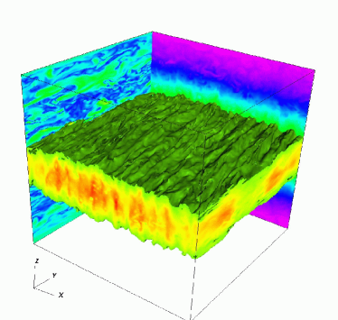
Figure 1.— Isosurface (at $\rho=0.75$) and slices of the density at 250 orbits in a domain of size $4H\times 4H\times 4H$ (S64Z4R4). On the left face of the domain a slice of the magnitude of the magnetic field is shown.

3. Results

3.1. Resolution Study

Our primary goal is to test the robustness of sustained turbulence and angular momentum transport in stratified shearing boxes with zero net flux, and in addition, to characterize the properties of the turbulence in this case. Figure 1 is an image showing the three-dimensional structure of the density at late time (250 orbits) in a typical simulation, computed with a resolution of 64 grid zones per scale height in an $4H\times 4H\times 4H$ domain. Spiral density waves characteristic of all simulations of the MRI in shearing boxes are evident in the density isosurfaces.

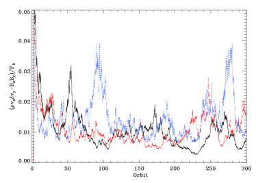
Figure 2.— Sum of integrated Reynolds and Maxwell stresses as a function of time in $H\times 4H\times 4H$ stratified shearing boxes. The curves represent the $128/H$ (black, solid), $64/H$ (red, dashed), and $32/H$ (blue, dotted) resolutions.

To investigate the convergence of the stress with numerical resolution, we have performed a resolution study at 32, 64 and 128 grid zones per scale height in an $H\times 4H\times 4H$ domain (hereafter S32R1Z4, S64R1Z4, and S128R1Z4, respectively). Since interest in MRI turbulence is driven primarily by its role in angular momentum transport, we first focus on stress as a diagnostic. Table 1 and Figure 2 summarize the behavior of the stress as we vary the resolution.

The MRI turbulence contributes to the stress through the Maxwell stress $-B_{x}B_{y}$ and the Reynolds stress $\rho v_{x}\delta v_{y}$, where $\delta v_{y}$ is the $y-$component of the velocity with background shear removed. The domain and time average of these quantities are listed in Table 1. We have normalized them by the initial midplane pressure $P_{0}$. Since the initial condition is in hydrostatic equilibrium and magnetic pressure is always significantly lower than gas pressure at the midplane (see e.g. Figure 6), this value of the midplane pressure does not evolve significantly. With this normalization they are roughly equivalent to the $\alpha$ parameter of Shakura & Sunyaev (1973). The time average is carried out from 50-300 orbits to exclude the transient period of enhanced turbulence during and immediately after the linear growth phase of the MRI.

Both contributions to the stress decrease as we increase resolution, but the changes are much smaller when going from $64/H$ to $128/H$ than from $32/H$ to $64/H$, indicating convergence. This should be compared with the behavior observed in unstratified boxes (e.g. Sano et al., 2004; Fromang & Papaloizou, 2007; Pessah et al., 2007) in which total stress decreases by factors of $\sim 2$ as resolution is increased by a factor of $2$. The normalized total stress in the S128R1Z4 run is $0.0095$, comparable to previous results for stratified domains with zero net flux (Brandenburg et al., 1995; Stone et al., 1996; Johansen et al., 2009; Suzuki & Inutsuka, 2009). The Maxwell stress is 4-5 times greater than Reynolds stress, which is slightly higher than, but roughly consistent with previous results for stratified domains (e.g. Stone et al., 1996). Similar values are also observed in unstratified runs, where the result appears to be independent of field geometry or flux, and depend mainly on the rate of shear (Pessah et al., 2006).

Table 1 also includes the rms toroidal field, volume averaged over the central two scale heights and time averaged from 50 orbits onward. The rms field strengths are relatively weak, with $\langle B_{y}\rangle^{2}\sim 0.01\langle B_{y}^{2}\rangle$, but may still be dynamically important since the presence mean toroidal field in unstratified simulations has been shown to enhance turbulence stresses and energy densities (Hawley et al., 1995). In fact, the rms toroidal field strength correlates well with the stress, although this may be the by-product of stronger turbulence rather than a cause.

Figure 3.— Comparison of magnetic energy density power spectra for $32/H$ (solid), $64/H$ (dotted), and $128/H$ (dashed) resolutions in $H\times 4H\times 4H$ stratified shearing boxes. Power spectra have been averaged over spherical shells of constant $k\equiv|{\mbox{\boldmath{$k$}}}|$ The $k^{3}$ normalization then makes the y ordinate proportional to the fractional contribution to the total power per logarithmic interval in $k$. The power spectra are time averaged from 50-300 orbits.

Figure 2 shows the temporal variation of the total stress. There is considerable variability, with relatively long-lived ($\gtrsim 50$ orbit) departures from the mean. In the S32R1Z4 run, the $\sim 50$ orbit periods of enhanced stress contribute almost as much to the average as the longer periods of ‘quiescent’ stress. There are similar long-term fluctuations in the higher resolution runs, but these are generally smaller in amplitude and less important for determining the overall mean. Nevertheless, it is clear that one must average over relatively long baselines to obtain a representative value, making higher resolutions prohibitively expensive.

A power spectral analysis of the magnetic field also indicates convergence, at least for the large scales where most of the power resides. Figure 3 shows the averaged PSD for the S32R1Z4, S64R1Z4, and S128R1Z4 simulations. We average over spherical shells in $k$-space (see §2.1) and in time, excluding the first 50 orbits to avoid the initial transients. There is a significant drop in power in going from the $32/H$ to $64/H$ resolution runs, combined with a shift in the peak of PSD to larger $k$. However, when going from $64/H$ to $128/H$, there is significantly smaller drop in amplitude at most scales and a much smaller shift in the peak wave number, also indicating convergence.

Figure 4.— Comparison of magnetic (solid) and kinetic (doted) energy density power spectra in the $128/H$ resolution, $H\times 4H\times 4H$ stratified shearing box.

Although we focus on the magnetic energy density, a similar convergence is observed in the PSD of the kinetic energy density. We show a comparison of the kinetic and magnetic energy density PSDs for run S128R1Z4 in Figure 4. It is notable that power in the magnetic field fluctuations exceeds that of the kinetic energy at all scales. This is in contrast to unstratified runs which typical show greater power in the kinetic energy at the lowest $k$, with magnetic energy dominating the power at higher $k$. It also differs from simulations of helically driven turbulence where the kinetic and magnetic energy have comparable amplitude at all but the lowest $k$ where magnetic energy dominates (Brandenburg, 2001).

The convergent behavior of the stratified runs should be contrasted with that of the unstratified simulations shown in Figure 5. This plot shows the PSD for four unstratified runs with resolutions of $32/H$, $64/H$, $128/H$, and $256/H$ in $H\times 4H\times H$ shearing boxes. Each factor of two increase in resolution results in a decrease by nearly a factor of two in the integrated power. There is also a shift in the peak wavenumber to larger $k$ as resolution increases. This lack of convergence is almost identical to the that found by previous authors (Fromang & Papaloizou, 2007; Guan et al., 2009; Simon et al., 2009). It seems that both the power and characteristic scale of the turbulence are set by the domain resolution. Adding stratification appears to fundamentally change the dynamics and provides a characteristic scale and amplitude of the turbulence which is independent of the resolution. This could be related to the different mechanisms that lead to the saturation of the MRI in the presence of stratification, perhaps associated with the development, and subsequent buoyant rise, of large scale magnetic fields (Pessah et al., 2007).

In Figure 6 we show spacetime diagrams for several variables associated with the magnetic field. For the sake of brevity, we focus on magnetic quantities, which appear to play the dominant role, as suggested by the PSD analysis above. The spacetime plots are generated by averaging over the $x$ and $y$ coordinates at each height in the domain every quarter of an orbit. The top panel of Figure 6 shows $\beta=2\langle P\rangle/\langle B^{2}\rangle$, where the angle brackets denote horizontal averages. As noted previously, magnetic pressure remains relatively weak near the midplane, but dominates in the surface regions ($|z|\gtrsim 1.5H$).

Figure 5.— Comparison of magnetic energy density power spectra for $32/H$ (solid), $64/H$ (dotted), $128/H$ (dashed), and $256/H$ (dot-dashed) resolutions in $H\times 4H\times H$ unstratified shearing boxes. Power spectra are time averaged from 60-100 orbits. The spectra peak at $kH/(2\pi)=$ 4, 7, 14, and 17, for the $32/H$, $64/H$, $128/H$, and $256/H$ runs respectively. This roughly consistent with a scaling $k_{\rm max}\simeq 2\pi(H\Delta)^{-1/2}$, where $\Delta$ is the spacing between grid zones.

The middle panels show the normalized $x$ and $y$ components of the magnetic field. The $B_{y}$ component is considerably larger than $B_{x}$ and they are negatively correlated. The symmetry of the boundary conditions and the initial conditions require the vertical average of these quantities to be zero. Nevertheless, there are localized regions of net field that, under the effects of buoyancy, trace out curved trajectories in the spacetime plot. This is similar to other ‘butterfly diagrams’ seen in previous shearing box calculations of stratified domains (Brandenburg et al., 1995; Stone et al., 1996; Turner, 2004; Johansen et al., 2009; Suzuki & Inutsuka, 2009). Consistent with previous simulations, the polarity is usually even about the midplane and, at fixed height, oscillates quasiperiodically on time scales of $\lesssim 10$ orbits.

Within the inner three scale heights, the horizontally averaged net field is a sum over a fluctuating $B$ field so that $\langle B_{y}\rangle^{2}$ is much less than $\langle B_{y}^{2}\rangle$ and similarly for $B_{x}$. As these regions of net field buoyantly rise, the ratio of $\langle B_{y}\rangle^{2}/\langle B_{y}^{2}\rangle$ increases. Near the vertical boundaries magnetic dominated regions of rather uniform ${\mbox{\boldmath{$B$}}}\sim B_{y}{\hat{\mbox{\boldmath{$j$}}}}$ develop. Their presence is very likely related to our assumption of periodicity in the vertical boundary condition, so they are likely not physically relevant to real accretion flows. The degree to which these regions affect the dynamics is discussed further in §3.2.

The bottom panel of Figure 6 shows the Maxwell stress. In addition to the temporal fluctuations, there is also considerable variation with height. The middle three scale heights dominate and regions of greatest stress tend to be found off the midplane. The stress is weakest in the magnetically dominated regions very near the boundary, and is even slightly negative in some places (although the colorbar only goes to zero). A striking result is the correlation of regions of stronger than average $\langle B_{y}\rangle$ with regions of larger than average stress. This lends support to the idea that the presence of a mean toroidal field leads to enhanced turbulent stresses and energy densities. Although not shown, we note that the spacetime plot of the Reynolds stress is very similar to the Maxwell stress and the two are well correlated in both $z$ and time.

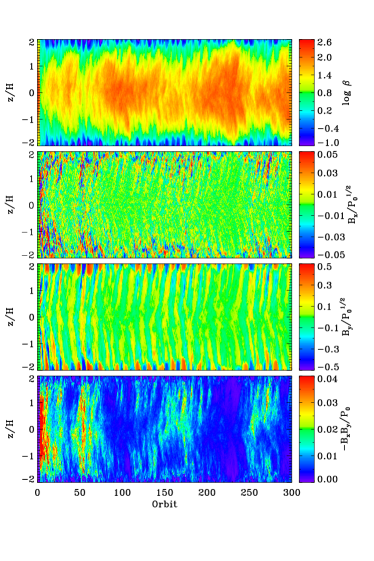
Figure 6.— Spacetime plot for the $128/H$ resolution run in a $H\times 4H\times 4H$ stratified shearing box. From top-to-bottom the panels show the horizontally averages of plasma $\beta$, the normalized radial and toroidal components of the magnetic field (respectively), and the Maxwell stress as a function of height above the midplane.

Figure 6 shows there is clearly a significant amount of large scale and long timescale structure in space and time coordinates, respectively. To better understand and quantify this structure, we perform a complimentary Fourier analysis in both space and time. Since we are interested in the structure of the horizontally averaged box, we focus on vertical $k$-vectors with ${\mbox{\boldmath{$k$}}}=k_{z}\hat{\mbox{\boldmath{$z$}}}$. Every one-quarter of an orbit, we compute the discrete Fourier transform $B^{2}(k_{z})\equiv 4\pi k_{z}^{2}|\tilde{B}(k_{z})|^{2}$, which is analogous to the $B^{2}_{k}$ defined in §2.1, but with $k_{z}$ replacing $k$. Note that the two quantities can differ significantly since the Fourier amplitudes are far from isotropic in $k$-space. For each $k_{z}$, we Fourier transform in time to obtain $B^{2}(k_{z},f)$ where $f$ is the time domain frequency. We divide the data into five 50 orbit time series (between 50 and 300 orbits), Fourier transform each separately, and then average. Although we lose access to the longest timescales, the averaging reduces the variance in the resulting power spectra, which are plotted in Figure 7.

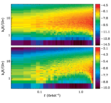
Figure 7.— Magnetic energy power spectra as function of both $k_{z}$ and $f$, where $f$ is the frequency in the time domain. The top and bottom panels correspond to the amplitudes of the $B_{x}$ and $B_{y}$ contributions the magnetic energy density, respectively. A detailed description is provided in the text (§3.1).

We plot both $\log[fk_{z}B^{2}_{x}(k_{z},f)/(2P_{0})]$ (top panel) and $\log[fk_{z}B^{2}_{y}(k_{z},f)/(2P_{0})]$ (bottom panel). Note that the horizontal average $\langle B_{z}\rangle$ is conserved (at zero) to round-off error, so there is no physical information in the $z$ component for vertical wavevectors. We have multiplied by both $k_{z}$ and $f$ before taking the logarithm. Since we use a logarithmic scale for both the $k_{z}$ and $f$ axes, this weights each pixel so that its color scales linearly with it contribution to the overall power (i.e. in the same sense that $\nu F_{\nu}$ is commonly used in astrophysics).

There are significant differences in the morphologies of the $B_{x}$ and $B_{y}$ power spectra. For large spatial scales (small $k_{z}$), both $B_{x}$ and $B_{y}$ show a double peaked profile with significant power at large ($\sim 10$ orbit) and small ($\lesssim 1$ orbit) timescales, although the small scales are subject to aliasing. The dip at intermediate scales is somewhat more pronounced and persists to somewhat larger $k_{z}$ for $B_{y}$ than for $B_{x}$. As we shift to larger $k_{z}$, the peak in $B_{x}$ broadens significantly and the dip goes away entirely. For $B_{y}$ there is a locus of maximum power which shifts to higher $k_{z}$ as $f$ increases from about 0.1 to 1 cycles per orbit.

3.2. Vertically Extended Domains

Due to the low densities and high magnetic field strengths near the vertical boundary that arise from stratification, increasing the vertical extent of the domain is particularly computationally expensive. Therefore, we performed our resolutions study in boxes with four vertical scale heights, which seemed suitable to get a separation between the midplane dynamics and the vertical boundary. In order to confirm that our results are not strongly dependent on this choice, we have repeated our $32/H$ resolution run with six vertical scale heights (hereafter S32R1Z6). As one can see in Table 1, the resulting volume average of the stress in the two $32/H$ simulations is in reasonable agreement, although slightly smaller in the S32R1Z6 run.

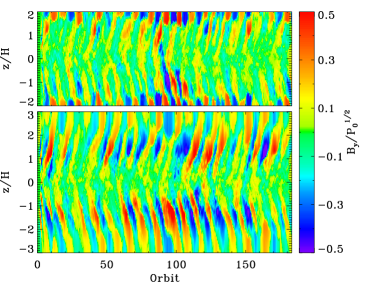
Figure 8.— Spacetime plot comparing the toroidal component of the magnetic field in stratified shearing boxes with $32/H$ resolution. The top and bottom panels show simulations with four and six scale height vertical extent (respectively).

One downside to choosing vertically periodic boundary conditions, is the buildup of strongly magnetized regions with uniform $B_{y}$ near the boundaries. Although these regions don’t contribute significantly to the angular momentum transport, they are likely unphysical so one might worry that they feedback on the dynamics closer to the midplane. In order to get a better sense of their effect on the flow, we have plotted spacetime diagrams comparing the S32R1Z4 and S32R1Z6 simulations in Figures 8 and 9.

Figure 8 shows the $y$ component of the magnetic field. In a larger domain, there are still regions of rather uniform $B_{y}$ near the vertical boundaries. They are somewhat more extended in height but with a slightly weaker net field. The regions of net $B_{y}$ generated near the midplane can buoyantly rise to larger heights before interacting with the boundary region. Since the horizontally averaged field tends to increase as the fluid rises, this lead to further enhancement of the field strength over those found in the smaller domain.

Figure 9 shows the Maxwell stress in the two runs. In the central four scale heights the two plots look very similar, suggesting that the four scale height runs are yielding a fairly robust estimate for the angular momentum transport. Regions of enhanced Maxwell stress are again correlated with regions of strong net $B_{y}$. Similarly, the Maxwell stress is generally larger in the inner four scale heights than in the S32R1Z4 run. Note that the volume weighted average stresses in Table 1 are lower for S32R1Z6 than for S32R1Z4 because we are averaging over the whole box, including the regions of weak stress near the boundaries. If we restrict the averaging to the inner two scale heights for both the S32R1Z6 and S32R1Z4 runs, the time averaged Maxwell stress in the S32R1Z6 simulation is greater by about 10%.

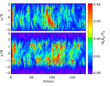
Figure 9.— Spacetime plot comparing the Maxwell stress in stratified shearing boxes with $32/H$ resolution. The top and bottom panels show simulations with four and six scale height vertical extent (respectively).

3.3. Radially Extended Domains

For the sake of computational expediency, we have performed our resolution study on domains with only one scale height in the radial direction. This has traditionally been the box size employed in most shearing box computations, mostly due to CFL constraints on the timestep which are imposed by the background shear. Using Athena’s orbital advection scheme (discussed in §2), we can consider larger domains to examine the effect of this choice on our results. We have computed shearing boxes with $4H\times 4H\times 4H$ domains at $32/H$ and $64/H$ resolution (hereafter S32R4Z4 and S64R4Z4, respectively).

We plot the evolution of the total stress in these two simulations in Figure 10 and the normalized, time and volume averaged stresses are listed in Table 1. The mean values of the stress are very similar to each other and also to those found at higher resolutions runs in the smaller boxes (S64R1Z4 and S128R1Z4). This suggest that convergence is occurring at even lower resolution than in the smaller domain computations. The time evolution differs from that seen in Figure 2 in that the amplitude of fluctuations is much lower.

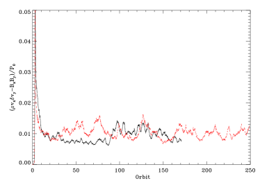
Figure 10.— Sum of box integrated Reynolds and Maxwell stresses as a function of time in $4H\times 4H\times 4H$ stratified shearing boxes. The curves represent the $64/H$ (black, solid) and $32/H$ (red, dashed) resolutions.

In Figure 11 we compare the PSDs from simulations with different radial extent but the same resolution (S64R1Z4 and S64R4Z4). The PSDs are very similar at all but the lowest $k$. At low $k$ the differences are accounted for in part by our shell averaging scheme. Since the larger box is a $4H$ cube, we can isotropically average shells all the way to $k=\pi/(2H)$. Since we can not do this average isotropically with smaller box, some of this low $k<2\pi/H$ power is included in the $k=2\pi/H$ bin. Overall, the PSDs seem to be rather independent of the aspect ratio, consistent with nearly identical values for the the box integrated stresses.

Figure 12 shows the spacetime diagram for the S64R4Z4 run. Overall, it is rather similar to S128R1Z4 spacetime diagram in Figure 6. There are long timescale ($\gtrsim 50$ orbit) fluctuations in the Maxwell stress, as well as $\sim 10$ orbit quasi-periodic variations in $B_{y}$ and Maxwell stress which are qualitatively similar to those in Figure 6. However, the amplitude of fluctuations is generally smaller in the larger box, consistent with the lower amplitude fluctuations in the total stress found in Figure 10.

Figure 11.— Comparison of magnetic energy density power spectra in stratified shearing boxes with $64/H$ resolution for domains with $L_{x}=4H$ (solid) and $L_{x}=H$ (dotted). The larger radial extent in the former allows one to isotropically average shell to lower $k$.

In order to better understand the lower fluctuation amplitudes, we have split the larger domain into four sub-domains of one scale height each in the radial direction. We find that the volume averaged stresses in each subdomain are highly correlated with each other. Therefore, the lower amplitude is not simply the result of “averaging” over several independent boxes, but appears to be a global property of a correlated domain. This behavior is somewhat surprising in light of the results of Guan et al. (2009), which show that the turbulence decorrelates on scales $\gtrsim H$ in unstratified boxes.

To investigate the correlation in stratified boxes, we have followed Guan et al. (2009) and calculated the trace of the two-point correlation of the magnetic field

$$\xi_{B}=\langle\delta B_{i}({\mbox{\boldmath{$x$}}})\delta B_{i}({\mbox{\boldmath{$x$}}}+\Delta{\mbox{\boldmath{$x$}}})\rangle$$ (19)

where $\delta B_{i}=B_{i}-\langle B_{i}\rangle$ and there is an implied summation over $i$. We computed the average in two ways: using the full domain and using only the innermost two scale heights. The two different procedures give different results for the correlations in the $x-y$ plane at large separations, since full domain average is dominated by the magnetically dominated regions near the vertical boundary. Since these are likely unphysical, we report only the two scale height average.

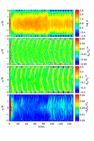
Figure 12.— Spacetime plot for the $64/H$ resolution run in a $4H\times 4H\times 4H$ stratified shearing box. From top-to-bottom the panels show the horizontally averages of plasma $\beta$, the normalized radial and toroidal components of the magnetic field (respectively), and the Maxwell stress as a function of height above the midplane.

We compute the correlation for 21 and 18 evenly spaced snapshots for for the S64R1Z4 (50-300 orbits) and S64R4Z4 (50-150 orbits) simulations, respectively. Although correlation at small separations is relatively consistent from snapshot to snapshot, there is significant variation at larger scales. Therefore, we average over all snapshots to get a mean correlation for each run. We plot the results of the two scale height average for the $x-y$ plane in Figure 13. For both simulations we normalize $\xi_{B}$ by their maximum values, $\xi_{0}$, which agree to within 10%. Our results are qualitatively consistent with those of Guan et al. (2009) in that we find comparable tilt angles $\theta_{t}$, which is the angle between the major axis of the correlation and the azimuthal axis. The correlation is very similar in both simulations, although the tilt angle from the S64R4Z4 calculation is slightly smaller ($\theta_{t}\sim 15^{\circ}$ rather than $18^{\circ}$).

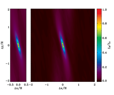
Figure 13.— Two-point correlation functions for the magnetic field in the $x-y$ plane. The axis labels $x$ and $y$ refer to the $\Delta x$ and $\Delta y$ implicit in (19). We have normalized the $\xi_{B}$ by it’s maximum value which occurs at $\Delta x=\Delta y=0$. The left and right panels correspond to the S64R1Z4 and S64R4Z4 calculations, respectively.

We also plot the correlation along the minor axis (defined by $\hat{\mbox{\boldmath{$x$}}}\cos\theta_{t}+\hat{\mbox{\boldmath{$y$}}}\sin\theta_{t}$) in Figure 14. Again, the core of the correlation at small separations is nearly identical in the two simulations and consistent with the results of Guan et al. (2009). Near $\Delta l\sim 0.1H$ the slope of the curve from the S64R1Z4 run flattens and the large scale correlation plateaus at a value of $\xi_{B}\simeq 0.04\xi_{0}$. The S64R4Z4 curve declines further, also flattens with $\xi_{B}\simeq 0.01\xi_{0}$ until $\Delta l\sim 1.3H$ where it drops nearly to zero.

As equation (19) requires, we have subtracted the mean field which is generally non-zero when only the inner two scale heights are considered (see Table 1), but is identically zero when using the whole domain. These mean fields can be substantial and would dominate the large scale correlation if included. It seems that these fields are sufficient to enforce relative uniformity in the magnetic energy and Maxwell stress throughout the four scale height domain. This uniformity may disappear for sufficiently large domains, and we see some suggestion of this in a calculations at $32/H$ resolution where we have compared $8H\times 8H\times 4H$ and $4H\times 4H\times 4H$ domains. Although we find that in both cases the Maxwell stress and magnetic energy density in one scale height wide subdomains remain correlated, they show greater variance in the the eight subdomains of the large box than in the four subdomains of the smaller box.

Figure 14.— Magnetic field correlation along the minor axis in the $x-y$ plane, plotted for S64R4Z4 (solid) and S64R1Z4 (dotted). For the horizontal axis, $\Delta l$ is the displacement from $\Delta x=\Delta y=0$ along the minor axis of the correlation.

3.4. Domains with Finite Dissipation

It has been shown that the behavior of MRI turbulence in unstratified shearing boxes depends on the nature of the dissipation (Sano et al., 1998; Fleming et al., 2000; Fromang et al., 2007; Lesur & Longaretti, 2007; Simon & Hawley, 2009). Simulations with explicit dissipation yield different results than those with only numerical dissipation, and the strength and evolution of the turbulence depends on both the viscosity $\nu$ and resistivity $\eta$, or equivalently the the Reynolds number $Re\equiv c_{s}H/\nu$ and the magnetic Reynodls number $Rm\equiv c_{s}H/\eta$. Specifically, it has been shown that $Re$ and $Rm$, or alternatively the magnetic Prandtl number $Pm=Rm/Re$, determine whether turbulence is sustained in zero net flux, unstratified simulations (Fromang et al., 2007; Simon & Hawley, 2009).

To see if these results hold in stratified domains, we perform three simulations with differing values of viscosity and resistivity: Re=800 with Pm=4 (hereafter Re800Pm4), Re=800 with Pm=2 (Re800Pm2), and Re=1600 with Pm=2 (Re1600Pm2). Examination of Figure 11 of Fromang et al. (2007) or Table 1 of Simon & Hawley (2009) show that none of these would sustain turbulence in an unstratified domains with no net field, regardless of whether Zeus or Athena is used for the simulations. We have confirmed these results for unstratified domains with our own Athena calculations.

Figure 15 shows the stress as a function of time for the three simulations with a logarithmic vertical scale. The behavior of Re800Pm4 and Re1600Pm2 is rather different from the unstratified domains where the simulations decay rapidly to zero on timescales of 10-20 orbits after the initial linear growth of the MRI. Even Re800Pm2, which drops rapidly to a dimensionless stress of $\sim 10^{-3}$ and then $\sim 10^{-4}$ in the stratified domain, decays much more rapidly and continues to even lower values in the unstratified domain. The behavior of the stratified domains is also considerably more complicated. Turbulence never decays away completely, but vigorous turbulence is not sustained in any of the calculations for longer than 100 orbits. The amplitude of variability is large, and turbulence decays slowly on timescales of hundreds of orbits. The Re1600Pm2 and Re800Pm2 runs both show a recovery nearly to peak values after spending over 100 orbital periods in stagnation or slow decay!

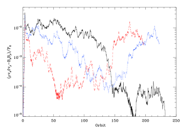
Figure 15.— Sum of box integrated Reynolds and Maxwell stresses as a function of time in stratified shearing boxes with explicit dissipation. The curves represent computations with Re=800, Pm=4 (black, solid); Re=1600, Pm=2 (blue, dotted) Re=800, Pm=2 (red, dashed).

Using the criteria of Fromang et al. (2007), we would probably have labeled the Re800Pm4 run as having sustained turbulence (over the first 100 orbits, which is the baseline used there), the Re1600Pm2 run as marginal, and the Re800Pm4 as either marginal or not having sustained turbulence, although the complex variability of the stratified runs makes this somewhat subjective. Figure 11 of Fromang & Papaloizou (2007) maps out a locus of sustained turbulence in Re – Pm space, and it’s notable that Re800Pm4 and Re1600Pm2 simulations are on the cusp of showing sustained turbulence while Re800Pm2 more firmly in the non-turbulent regime. Therefore, it would seem that stratification slightly increases the parameter space for which sustained turbulence is possible, but does not qualitatively alter the conclusion that turbulence dies out for sufficiently low Pm or sufficiently high Re.

It is suggestive that all three sets of dissipation terms show sustained turbulence in unstratified boxes once a net toroidal field is imposed (Simon & Hawley, 2009). As noted previously, it is conceivable that main impact of stratification is the production of toroidal field, which then lead to enhanced turbulence. The turbulence in the stratified runs is significantly less vigorous, but this may be consistent with the rms field strengths in the stratified simulations being much weaker than the toroidal fields considered by Simon & Hawley (2009),

In Figure 16 we plot the time average power spectra of the magnetic energy density from Re800Pm4 and Re1600Pm2, including S64R1Z4 for comparison. Since the magnetic energy in the Re1600Pm2 drops rapidly to a low amplitude, we have elected to exclude it. Of course, the amplitude of the power spectrum depends on the interval used in the time average, which is 25-100 orbits. The Re800Pm4 and Re1600Pm2 power spectra are similar in shape, falling off somewhat more rapidly than S64R1Z4 as $k$ increases.

The power in Re800Pm4 in exceeds that in Re1600Pm2 at all $k$. Note that these two calculations have the same resistivity but Re800Pm4 has a higher viscosity, so it has higher amplitude despite having larger overall dissipation (although this conclusion depends on the interval used for the comparison). Similar behavior is also observed in two-dimensional simulations of MRI driven turbulence with a vertical magnetic field and non-zero viscosity described in Masada & Sano (2008). In some of their runs saturation is not achieved since the turbulent stresses increase with time until the end of the runs. The fact that the magnetic field generated by the MRI can reach high amplitudes could be due to the viscous quenching of Kelvin-Helmholtz parasitic modes (Goodman & Xu, 1994; Pessah & Goodman, 2009). Although plausible, it is less obvious that this process is responsible for the similar behavior observed in the simulations with stratification and non-mean magnetic flux presented here.

Figure 16.— Comparison of magnetic energy density power spectra for computations with (solid, dotted) and without (dashed) explicit dissipation. The explicit dissipation curves correspond to computations with Re=1600, Pm=2 (solid) and Re=800, Pm=4 (dotted). Power spectra are time averaged from 25-100 orbits (with dissipation) or from 50-300 orbits (without dissipation).

4. Discussion

The numerical experiments presented here motivate two related questions: Why do the stratified simulations converge when the unstratified calculations clearly do not? What is the source of the dynamo cycles observed in the large scale fields? Answering the former requires detailed comparison with unstratified simulations, and will be the focus of future work. For the moment, we focus primarily on describing the large scale dynamo.

First, we compare with the discussion of Brandenburg et al. (1995), who noted the similarities of their stratified results with an $\alpha-\Omega$ dynamo model. They showed that the azimuthal EMF $\mathcal{E}_{y}=(\delta{\mbox{\boldmath{$v$}}}\times{\mbox{\boldmath{$B$}}})_{y}$ was correlated with the azimuthal field $B_{y}$ in a manner that leads to growth in the radial $B_{x}$. Coupled to the shear, which regenerates $B_{y}$ from $B_{x}$, this describes a simple dynamo.

Our results are in good agreement with their Equation (21). For the S128R1Z4 simulation, we find

$$\langle\mathcal{E}_{y}\rangle\simeq(-3,5)\times 10^{-3}\langle B_{y}\rangle\langle{\delta v}^{2}\rangle^{1/2},$$ (20)

where the values in parentheses correspond to volume averages one scale height above and below the midplane, respectively. They also report a correlation of $\langle\mathcal{E}_{x}\rangle$ with $\langle B_{y}\rangle$ in their Equation (22). Again, our results are qualitatively similar to theirs with

$$\langle\mathcal{E}_{x}\rangle\simeq(-1,1)\times 10^{-2}\langle B_{y}\rangle\langle{\delta v}^{2}\rangle^{1/2},$$ (21)

above and below the midplane. The first correlation confirms that there is a mechanism for regenerating the poloidal field from a toroidal field. The second relation suggests that $\langle\mathcal{E}_{x}\rangle$ generally acts to reduce the magnitude of $\langle B_{y}\rangle$ at the midplane, and is (at least partially) the result of buoyancy, as Brandenburg et al. (1995) discuss.

Figure 17.— Power spectra (top) and normalized EMFs (bottom) for a single oscillation period of S128R1Z4. The top panel shows PSDs $k|\tilde{B}_{x}(k_{0})|^{2}/(2P_{0})$ (solid) and $k|\tilde{B}_{y}(k_{0})|^{2}/(2P_{0})$ (dotted), where the former has been multiplied by a factor of 400 for plotting convenience. The bottom panel shows $e_{y,z}(k_{0})$ (solid), $e_{x,z}(k_{0})$ (dotted), and $s(k_{0})$ (dashed), which are defined in §2.1.

It’s instructive to examine this further with the Fourier analysis methods described in §2.1. We focus on the large scale field and consider the smallest vertically oriented vector ${\mbox{\boldmath{$k$}}}=k_{0}\hat{\mbox{\boldmath{$z$}}}=2\pi/L_{z}\hat{\mbox{\boldmath{$z$}}}$. Since, $k_{x}=k_{y}=0$, this term represents the Fourier amplitude of “horizontally averaged” quantities on the largest vertical scale. In Figure 17 we plot time variation of magnetic fields and EMFs over a single dynamo cycle for this choice of $k$. The top panel shows the Fourier amplitudes of magnetic energy densities $|\tilde{B}_{x}(k_{0})|^{2}$ (solid) and $|\tilde{B}_{y}(k_{0})|^{2}$ (dotted) for this wave vector. We have multiplied $|\tilde{B}_{x}(k_{0})|^{2}$ by a factor of 400 to plot both on the same scale. There is considerable variation from cycle to cycle, and Figure 7 shows that these oscillations are only quasiperiodic with a broad range of power for periods near 10 orbits, depending somewhat on the wavenumber used for the analysis. Nevertheless, this example is typical in that the curves are out of phase with a more uniform variation in $|\tilde{B}_{y}(k_{0})|^{2}$ than in $|\tilde{B}_{x}(k_{0})|^{2}$.

The bottom panel shows the corresponding right hand side quantities in (10) and (11), which, along with numerical dissipation, drive the evolution of the Fourier amplitudes. We normalize these quantities with the power spectra as described in §2.1, e.g. $e_{y,z}(k_{0})=2E_{y,z}(k_{0})/(|\tilde{B}_{x}(k_{0})|^{2}\Omega)$. We plot $e_{y,z}$ (solid), $e_{y,z}$ (dotted), and $s$ (dashed). Note that $e_{z,y}(k_{0})$ and $e_{z,x}(k_{0})$ are zero for $k_{0}$ because of the periodic boundaries. The shear term $s$ primarily drives the variation of $|\tilde{B}_{y}(k_{0})|^{2}$, flipping sign as $|\tilde{B}_{x}(k_{0})|^{2}$ goes to zero. In contrast, $e_{x,z}$ is generally negative, acting as turbulent resistivity. The $e_{y,z}(k_{0})$ term is more erratic, frequently flipping sign over a single cycle, but the net effect is an overall oscillation of $|\tilde{B}_{x}(k_{0})|^{2}$ over $\sim 7$ orbital periods.

In many respects, the behavior we see in the stratified simulations is similar to that observed in the unstratified, zero-net flux calculations of Lesur & Ogilvie (2008). Using an incompressible spectral code, they find dynamo cycles with a $\sim 5$ orbit periodicity. This is similar to the oscillations in our stratified runs where rms power on large scales is broadly distributed on times scales $\sim 6-10$ orbits (see Figure 7). The normalized quantities plotted in Figure 17 are equivalent to their Equation (16). Comparison of Figure 17 with Figs. 4 and 5 in their paper, show that the behavior of the EMFs during oscillations are also quite similar, suggesting that a common (or, at least, related) mechanism may be responsible for these oscillations. This motivates a more detailed comparison between unstratified and stratified runs in future work.

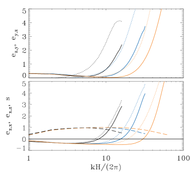
Figure 18.— Time averaged and normalized EMFs for $x$ (top panel) and $y$ (bottom panel) components of the induction equation. The curves correspond to the S32R1Z4 (black), S64R1Z4 (blue), and S128R1Z4 (red) calculations. In the top panel we plot $e_{z,y}(k)$ (solid) and $e_{y,z}(k)$ (dotted). The curves in the bottom panel are $e_{z,x}(k)$ (solid), $e_{x,z}(k)$ (dotted), and $s$ (dashed). With this normalization, curves for different simulations lie nearly on top of each other at low $k$. All quantities have been averaged from 50 to 300 orbits.

Although it is useful to focus on the vertical wave vectors when trying to understand properties of large scale fields, an understanding of the overall power spectrum benefits from an analysis of the shell integrated quantities. We plot the time and shell average EMFs terms in Figure 18 for S32R1Z4 (black) S64R1Z4 (blue), and S128R1Z4 (red). As in Figure 17, these quantities are normalized by the shell integrated power spectra. Each normalized term is then time averaged from 50-300 orbits. Since the amplitudes of the magnetic energy densities seem to be in statistical steady states over this period, we presume the left hand sides of (10) and (11) are nearly zero. Therefore the sum of the terms in each panel must be balanced by numerical dissipation terms, as discussed in previous work (Fromang & Papaloizou, 2007; Simon et al., 2009).

In the top panel we plot the terms $e_{z,y}(k)$ (solid) and $e_{y,z}(k)$ (dotted) which contribute to evolution of $B_{x}$. At the large scales, we find that the $e_{z,y}$ term is more important for field generation and its normalized amplitude is nearly independent of resolution. The $e_{y,z}$ term is smaller in amplitude and slightly negative as large scales. Even though $e_{y,z}$ tends to oscillates about zero over an individual dynamo cycle while $e_{z,y}$ usually remains positive, the amplitude of $e_{z,y}$ is generally larger, so the dominance of $e_{z,y}$ at large scales is not simply the result of time averaging. As one moves to smaller scales, $e_{y,z}$ rises and eventually dominates the generation of $B_{x}$. The characteristic wavenumber at which the crossing occurs shifts to higher values as the resolution increases.

The bottom panel shows $e_{z,x}(k)$ (solid), $e_{x,z}(k)$ (dotted) and $s$ (dashed), the terms which contribute growth in $B_{y}$. At large scales growth of $B_{y}$ is dominated by the shear term, while both $e_{z,x}$ and $e_{x,z}$ are of comparable magnitude and negative. At small scales, $e_{z,x}$ and $e_{x,z}$ both grow, becoming positive and dominating over the shear term. Again, the wavenumber of the crossover increases with resolution.

Authors have often focused on horizontally average properties of the flow or (equivalently) the power spectral variation only along vertical wave vectors (e.g Fromang & Papaloizou, 2007; Lesur & Ogilvie, 2008, which were discussed above). We note that the behavior of $e_{y,z}$ and $e_{z,y}$ we have described differs significantly from what one would infer if only vertical wavevectors were considered. As previously mentioned, the symmetries of the periodic box force $e_{z,y}(k_{z})$ to be zero, and only $e_{y,z}(k_{z})$ contributes. However, it is clear from Figure 18 that the vertical EMF and its toroidal variation is also essential for understanding the mechanism which sustains turbulence in these simulations.

The question remains as to why the addition of stratification leads to convergence in the turbulent stresses and energy densities. One possibility is that development of local toroidal field is key to sustaining turbulence in both stratified and unstratified domains. It is possible that the strength of toroidal field is entirely set by the resolution in unstratified domains, while stratified domains offer a characteristic scale which is independent of resolution, due to the action of the large scale dynamo. Indeed, it has already been demonstrated (e.g. Hawley et al., 1995; Simon & Hawley, 2009) that a global net toroidal field leads to enhanced turbulent energy densities and stresses, and leads to convergence in the stress as resolution increses (Guan et al., 2009). Furthermore, our simulations show a correlation between the stress and the strength of the mean toroidal field, both globally in the two scale height averages (Table 1) and locally in the spacetime plots (Figures 6 and 12). This hypothesis will be addressed further in future research, comparing in detail the results presented here with those from unstratified runs both with and without mean fields.

Due to our choice of periodic vertical boundaries, and our use of simplified thermodynamics, we have largely avoided detailed discussion of observational implications. Such questions are generally better addressed by studies which include more physically realistic vertical boundary conditions (e.g. Miller & Stone, 2000) or more realistic thermodynamics, including the treatment of radiation (e.g. Turner, 2004; Hirose et al., 2006). However, it is worth briefly noting that our work confirms some important results of earlier studies (see e.g. Brandenburg et al., 1995; Stone et al., 1996; Miller & Stone, 2000). Figures 3 and 6 show that a significant fraction of the magnetic energy in these simulations resides in large scale magnetic fields that rise buoyantly to the low density regions above the disk midplane. Blackman & Pessah (2009) argue that the magnetic field structures that power accretion disk coronae must be associated with characteristic lengths that are large compared to the typical turbulent eddies. If this were not the case, the timescales associated with turbulent diffusion would be smaller than the corresponding buoyant rise time, making it difficult to transport significant magnetic energy to the coronae. In other words, if the corona is a consequence of magnetic field structures that originate within the turbulent disk via the MRI (or other magnetic instabilities), but that dissipate above the disk midplane, then these structures must be of large enough scale to survive the buoyant rise without being shredded by the turbulence within the disk. Thus, the results presented in this paper provide support to the prevailing paradigm for X-ray emission in accreting systems which involves an optically thin, hot corona powered by the dissipation of magnetic fields (e.g. Haardt & Maraschi, 1993; Field & Rogers, 1993).

5. Conclusions

We have used Athena to examine the effects of stratification on magnetohydrodynamic turbulence driven by the magnetorotational instability. We have shown that stratified simulations converge as resolution increases, even in domains with zero-net-flux and no explicit dissipation. This is contrary to our own calculations of zero-net-flux unstratified domains, which do not converge, confirming previous results (Fromang & Papaloizou, 2007; Guan et al., 2009; Simon et al., 2009). We have also considered calculations with explicit dissipation, and confirmed previous results that the maintenance of sustained turbulence is magnetic Prandtl number dependent. Stratification appears to extend the range for which sustained turbulence develops, and may allow sustained turbulence at slightly lower Prandtl number for a given Reynolds number. However, the behavior is rather complex with larger variations and evolution on long timescales (greater than 100 orbits).

At the highest resolutions considered ($64/H$ and $128/H$) the ratio of total stress to midplane pressure has a mean value of $\alpha\sim 0.01$, but with considerable fluctuation about this mean on long ($\gtrsim 50$ orbit) timescales. Since real astrophysical systems are stratified, this somewhat alleviates concerns that magnetorotational turbulence might be unable to provide the required angular momentum transport in accretion disks, although values a factor of ten higher have been inferred in some astrophysical sources (King et al., 2007). Similarly, it partially alleviates concerns that explicit dissipation may be required in global disk simulations at high resolution, as stratification and net toroidal fields arise naturally in such calculations.

We have shown that these conclusions do not depend sensitively on the vertical or radial dimensions of the box. Domains with radial extents of one and four scale heights give the same time averaged values for $\alpha$ and have nearly identical power spectral densities for the magnetic energy. Stresses are somewhat more sensitive to variations in the vertical height of the domain, although this may be related to our assumptions of vertical periodicity. Increasing the vertical extent from four to six scale heights results in only a slight increase in the time and spatially averaged stresses, as long as the spatial average is carried out over the same volume (about 10% when using the inner two scale heights).

Our results generally reproduce the qualitative features found by previous authors for stratified systems (e.g. Brandenburg et al., 1995; Stone et al., 1996). This includes oscillations with a periods of $\lesssim 10$ orbits in which the horizontally averaged radial and toroidal fields alternate sign. Coupled with buoyancy this leads to a characteristic butterfly diagram in horizontally averaged space-time plots. A comparison of our results with those of Lesur & Ogilvie (2008) suggest the mechanisms for generating the large scale field oscillations in the stratified and unstratified domains may be related.

References

- Balbus & Hawley (1998) Balbus, S. A., & Hawley, J. F. 1998, Reviews of Modern Physics, 70, 1
- Blackman & Pessah (2009) Blackman, E. G., & Pessah, M. E. 2009, ArXiv: 0907.2068
- Bodo et al. (2008) Bodo, G., Mignone, A., Cattaneo, F., Rossi, P., & Ferrari, A. 2008, A&A, 487, 1
- Brandenburg (2001) Brandenburg, A. 2001, ApJ, 550, 824
- Brandenburg et al. (1995) Brandenburg, A., Nordlund, A., Stein, R. F., & Torkelsson, U. 1995, ApJ, 446, 741
- Field & Rogers (1993) Field, G. B., & Rogers, R. D. 1993, ApJ, 403, 94
- Fleming et al. (2000) Fleming, T. P., Stone, J. M., & Hawley, J. F. 2000, ApJ, 530, 464
- Fromang & Papaloizou (2007) Fromang, S., & Papaloizou, J. 2007, A&A, 476, 1113
- Fromang et al. (2007) Fromang, S., Papaloizou, J., Lesur, G., & Heinemann, T. 2007, A&A, 476, 1123
- Gardiner & Stone (2005) Gardiner, T. A., & Stone, J. M. 2005, Journal of Computational Physics, 205, 509
- Gardiner & Stone (2008) —. 2008, Journal of Computational Physics, 227, 4123
- Goodman & Xu (1994) Goodman, J., & Xu, G. 1994, ApJ, 432, 213
- Guan et al. (2009) Guan, X., Gammie, C. F., Simon, J. B., & Johnson, B. M. 2009, ApJ, 694, 1010
- Haardt & Maraschi (1993) Haardt, F., & Maraschi, L. 1993, ApJ, 413, 507
- Hawley et al. (1995) Hawley, J. F., Gammie, C. F., & Balbus, S. A. 1995, ApJ, 440, 742
- Hirose et al. (2006) Hirose, S., Krolik, J. H., & Stone, J. M. 2006, ApJ, 640, 901
- Johansen et al. (2009) Johansen, A., Youdin, A., & Klahr, H. 2009, ApJ, 697, 1269
- Johnson et al. (2008) Johnson, B. M., Guan, X., & Gammie, C. F. 2008, ApJS, 177, 373
- King et al. (2007) King, A. R., Pringle, J. E., & Livio, M. 2007, MNRAS, 376, 1740
- Lesur & Longaretti (2007) Lesur, G., & Longaretti, P.-Y. 2007, MNRAS, 378, 1471
- Lesur & Ogilvie (2008) Lesur, G., & Ogilvie, G. I. 2008, A&A, 488, 451
- Masada & Sano (2008) Masada, Y., & Sano, T. 2008, ApJ, 689, 1234
- Masset (2000) Masset, F. 2000, A&AS, 141, 165
- Miller & Stone (2000) Miller, K. A., & Stone, J. M. 2000, ApJ, 534, 398
- Pessah et al. (2006) Pessah, M. E., Chan, C.-K., & Psaltis, D. 2006, MNRAS, 372, 183
- Pessah et al. (2007) Pessah, M. E., Chan, C.-k., & Psaltis, D. 2007, ApJ, 668, L51
- Pessah & Goodman (2009) Pessah, M. E., & Goodman, J. 2009, ApJ, 698, L72
- Sano et al. (1998) Sano, T., Inutsuka, S.-I., & Miyama, S. M. 1998, ApJ, 506, L57
- Sano et al. (2004) Sano, T., Inutsuka, S.-i., Turner, N. J., & Stone, J. M. 2004, ApJ, 605, 321
- Shakura & Sunyaev (1973) Shakura, N. I., & Sunyaev, R. A. 1973, A&A, 24, 337
- Simon & Hawley (2009) Simon, J. B., & Hawley, J. F. 2009, ArXiv: 0906.5352
- Simon et al. (2009) Simon, J. B., Hawley, J. F., & Beckwith, K. 2009, ApJ, 690, 974
- Sorathia et al. (2009) Sorathia, K., Reynolds, C. S., & Armitage, P. J. 2009, ApJ, submitted
- Stone & Gardiner (2009) Stone, J. M. & Gardiner, T. A. 2009, ApJ, submitted
- Stone et al. (2008) Stone, J. M., Gardiner, T. A., Teuben, P., Hawley, J. F., & Simon, J. B. 2008, ApJS, 178, 137
- Stone et al. (1996) Stone, J. M., Hawley, J. F., Gammie, C. F., & Balbus, S. A. 1996, ApJ, 463, 656
- Suzuki & Inutsuka (2009) Suzuki, T. K., & Inutsuka, S.-i. 2009, ApJ, 691, L49
- Turner (2004) Turner, N. J. 2004, ApJ, 605, L45