Fullerenes, Zero-modes, and Self-adjoint Extensions

Abstract

We consider the low-energy electronic properties of graphene cones in the presence of a global Fries-Kekulé Peierls distortion. Such cones occur in fullerenes as the geometric response to the disclination associated with pentagon rings. It is well known that the long-range effect of the disclination deficit-angle can be modelled in the continuum Dirac-equation approximation by a spin connection and a non-abelian gauge field. We show here that to understand the bound states localized in the vicinity of a pair of pentagons one must, in addition to the long-range topological effects of the curvature and gauge flux, consider the effect the short-range lattice disruption near the defect. In particular, the radial Dirac equation for the lowest angular-momentum channel sees the defect as a singular endpoint at the origin, and the resulting operator possesses deficiency indices $(2,2)$. The radial equation therefore admits a four-parameter set of self-adjoint boundary conditions. The values of the four parameters depend on how the pentagons are distributed and determine whether or not there are zero modes or other bound states.

I Introduction

The essential features of the valance and conduction bands of planar graphene [1] can be modelled as a pair of 2+1 dimensional Dirac fermions, one for each of the conical band touchings that occur at the points ${\bf k}={\bf K}$ and ${\bf k}={\bf K}^{\prime}$ in the Brillouin zone [2]. A Fries [3] (or equivalently Clar [4]) Kekulé-structure distortion of the hexagonal graphene lattice will couple the two Dirac points and introduce a mass gap. If the phase of the ${\bf K}$-${\bf K}^{\prime}$ coupling can vary with position, there may exist topologically stable vortex textures that are associated with zero modes and charge fractionalization [5, 6, 7].

A complex-valued ${\bf K}$-${\bf K}^{\prime}$ coupling is unlikely to occur spontaneously as a result of a simple Peierls distortion – although it might be artificially engineered through proximity-effect coupling to vortices in a superconducting substrate [7, 8]. An alternative and naturally occurring form of vortex may be provided by local curvature-inducing geometric defects such as pentagons and heptagons [9, 10, 11, 12]. A spherical fullerene such as C₆₀ possesses twelve pentagonal defects and, even in the absence of Kekulé distortion, its energy spectrum contains six delocalized low-energy levels. These near-zero-energy levels have long been understood as the lattice relicts of six exactly zero-energy modes of the continuum Dirac hamiltonian [13, 14]. The continuum zero-modes are those predicted by the index theorem for 2+1 dimensional Dirac fermions moving in a fictitious monopole magnetic field that mimics the effect of the defects. One quarter of a Dirac unit of monopole flux threads through each of the twelve pentagons, and for C₆₀ this discretely-lumped field is sufficiently spread out that the resulting energy spectrum is well approximated by a spatially uniform field [13, 14]. There are three units of flux altogether, and so the index theorem predicts three zero modes apiece for the two Dirac fermion species of planar graphene.

The fictitious flux through the closed surface of the fullerene molecule means that when the discrete lattice hamiltonian is approximated by two continuous-space Dirac hamiltonians, the continuum wavefunctions must be regarded as sections of a twisted line bundle, the twist being characterized by a Chern number of $\pm 3$. When a purely real Kekulé field is introduced on the fullerene, the threefold twist, when coupled with a natural choice of how we introduce the gauge holonomy, allows the real ${\bf K}$-${\bf K}^{\prime}$ coupling matrix elements to be perceived by the continuum approximation as being associated with a charge-$2$ complex Higgs field possessing a net winding number of six. Each pair of pentagons is then effectively a single vortex, and each such vortex should, by the Jackiw-Rossi-Weinberg index theorem [15, 16], contain at least one zero mode. The six low-lying “zero modes” should therefore survive the introduction of the Kekulé induced mass gap, and, in theory, its principal effect should be to localize the previously extended states in the vicinity of the pentagonal defects.

In practice, numerical investigation of the lattice spectrum [11] shows that although the “zero modes” are not immediately destroyed by the introduction of the Kekulé Higgs field, their energy is affected. Indeed as the ratio $h$ of the double bond to single bond hopping evolves from zero to large values the “zero-modes” cross the finite-size gap from the negative to the positive part of the spectrum. What was not obvious from the plots in [11] is that at the same time the zero-mode wavefunctions evolve from being tightly localized around the defects to being antilocalized. Thus these modes, while still topologically interesting, are not acting as expected from the continuum Jackiw-Rossi-Weinberg index theorem. This theorem predicts that the energy of the zero modes will be unaltered by the introduction of the Higgs field, and that they will be localized for any sign of the mass.

In this paper we will explore what feature of the continuum approximation to the lattice hamiltonian is responsible for this behaviour. We will focus on isolated pentagons and isolated pairs of pentagons. These disinclination defects roll the sheet of graphene into a cone. Away from the tip of the cone the geometry is locally flat and a continuum twisted Dirac hamiltonian approximation should be reliable. Near the tip, the exact form of the lattice becomes important. The lattice effects can be accounted for, however, by imposing a boundary condition on the continuum wavefunction at the tip of the cone. The result is the introduction of a four-parameter family of self-adjoint extensions to the Dirac operator. General values of the extension parameters explicitly break the symmetry required for the index theorem, and suitable choices of the parameters reproduce the numerically observed phenomena.

II Planar graphene and the Dirac equation

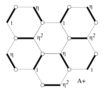
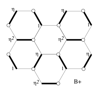
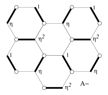
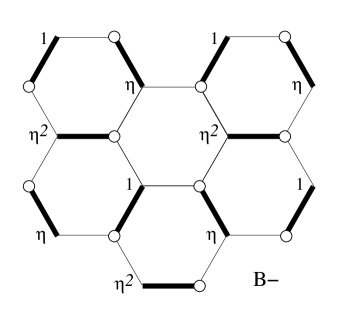
Figure 1: The zero-energy reference states ${|A+\rangle}$, ${|B+\rangle}$, ${|A-\rangle}$ and ${|B-\rangle}$. The empty circles indicate that the wavefunction is zero at those sites. The symbols $\eta$ and $\eta^{2}$ indicate that the wavefunction takes the values $\eta=\exp(2\pi i/3)$ and $\eta^{2}=\bar{\eta}=\exp(-2\pi i/3)$ at that site. The heavy lines indicate a Fries stucture of “double” bonds, whose hopping will increase from $t$ to $t+\delta t$ when a Peierls distortion occurs.

In order to establish our notation, we begin with a quick review of how the tight-binding (Hückel) approximation [13] for planar graphene leads to a massive Dirac hamiltonian. In this approximation the $\pi$ electrons hop on a two-dimensional honeycomb lattice with lattice constant $a$. The honeycomb lattice is bipartite with the property that nearest-neighbour hopping takes an electron from sublattice A to sublattice B, and vice versa. We denote the hopping amplitude between nearest neighbour sites in undeformed graphene by $t$. A Kekulé structure is an assignment to the lattice edges of a pattern of single and double bonds such that each carbon atom partakes of two single bonds and one double bond. There are in general many such assignments, but patterns that lead to a maximum number of benzene-like hexagons are known as Fries structures. Fullerenes that possess a globally defect-free Fries structure (the so-called leapfrog fullerenes [17]) are typically the most chemically stable. This is because a spontaneous Peierls distortion that shortens the Fries-structure double bonds and increases their hopping amplitude from $t$ to $t+\delta t$ will open a gap between the highest occupied molecular orbital (HOMO) and the lowest unoccupied molecular orbital (LUMO), lower the energy of the system, and give the molecule the property of having a “closed shell.” Such a spontaneous distortion occurs in C₆₀ where the double bonds have length $\sim$ 0.1388 nm while the single bonds have length $\sim$ 0.1432 nm [18].

The hopping hamiltonian for the undistorted infinite lattice has four linearly independent zero-energy eigenstates which are displayed in figure 1. The labels A and B indicate that the non-zero amplitudes are supported on sublattice A or B respectively, and the “+” and ‘$-$” configurations have opposite handedness in the way that their complex phases evolve as we circle the zero sites. Both “+” configurations have the same lattice momentum ${\bf k}={\bf K}$ and both “$-$” configurations have lattice momentum ${\bf K}^{\prime}$. Any low energy eigenfunction will be a slowly varying linear combination

$$\Psi({\bf r})=f_{A+}({\bf r}){\langle{\bf r}|A_{+}\rangle}+f_{B+}({\bf r}){\langle{\bf r}|B_{+}\rangle}+f_{A-}({\bf r}){\langle{\bf r}|A_{-}\rangle}+f_{B-}({\bf r}){\langle{\bf r}|B-\rangle}$$ (1)

of these reference wavefunctions. Here ${\bf r}$ labels discrete lattice points, but since the $f({\bf r})$ are to be slowly varying on the scale of the lattice they can be regarded as being smooth continuum functions ${\mathbb{R}}^{2}\to{\mathbb{C}}$.

The hamiltonian acts on the array of slowly varying functions $f$ as

$$H\left(\matrix{f_{A+}\cr f_{B+}\cr f_{B-}\cr f_{A-}}\right)={3at\over 2}\left(\matrix{0&-2\partial_{z}&0&0\cr 2\partial_{{\bar{z}}}&0&0&0\cr 0&0&0&2\partial_{z}\cr 0&0&-2\partial_{{\bar{z}}}&0}\right)\left(\matrix{f_{A+}\cr f_{B+}\cr f_{B-}\cr f_{A-}}\right),$$ (2)

where

$$\partial_{z}\equiv{\partial\over\partial z}={1\over 2}\left({\partial\over\partial x}-i{\partial\over\partial y}\right),\quad\partial_{\bar{z}}\equiv{\partial\over\partial{\bar{z}}}={1\over 2}\left({\partial\over\partial x}+i{\partial\over\partial y}\right).$$ (3)

When the hopping is modified by the Fries-Kekulé structure shown in figure 1, the reference states are no longer exactly zero-energy eigenfunctions. Instead $H{|A+\rangle}=\delta t{|B-\rangle}$ and $H{|A-\rangle}=\delta t{|B+\rangle}$. Non-zero matrix elements therefore appear coupling the ${\bf K}$ Dirac point to the ${\bf K}^{\prime}$ point:

$$H(\Phi)\left(\matrix{f_{A+}\cr f_{B+}\cr f_{B-}\cr f_{A-}}\right)={3at\over 2}\left(\matrix{0&-2\partial_{z}&\Phi&0\cr 2\partial_{{\bar{z}}}&0&0&\Phi\cr\Phi&0&0&2\partial_{z}\cr 0&\Phi&-2\partial_{{\bar{z}}}&0}\right)\left(\matrix{f_{A+}\cr f_{B+}\cr f_{B-}\cr f_{A-}}\right),$$ (4)

where $\Phi=(2/3at)\delta t$. The derivative blocks can be written as

$$\left(\matrix{0&-2\partial_{z}\cr 2\partial_{\bar{z}}&0}\right)=-i\sigma_{2}{\partial\over\partial x}+i\sigma_{1}{\partial\over\partial y}=\tilde{\mbox{\boldmath$\sigma$}}\cdot{\bf p},$$ (5)

where $\tilde{\mbox{\boldmath$\sigma$}}\equiv(\sigma_{2},-\sigma_{1})$ is a 90^∘ rotated version of the ${\mbox{\boldmath$\sigma$}}=(\sigma_{1},\sigma_{2})$ spin vector.

We can if, we prefer, write

$$H(\Phi)\left(\matrix{if_{A+}\cr f_{B+}\cr if_{B-}\cr f_{A-}}\right)={3at\over 2}\left(\matrix{0&-2i\partial_{z}&\Phi&0\cr-2i\partial_{{\bar{z}}}&0&0&\Phi\cr\Phi&0&0&2i\partial_{z}\cr 0&\Phi&2i\partial_{{\bar{z}}}&0}\right)\left(\matrix{if_{A+}\cr f_{B+}\cr if_{B-}\cr f_{A-}}\right),$$ (6)

in which case the derivative blocks involve the more familiar form

$$\left(\matrix{0&-2i\partial_{z}\cr-2i\partial_{\bar{z}}&0}\right)=-i\sigma_{1}{\partial\over\partial x}-i\sigma_{2}{\partial\over\partial y}={\mbox{\boldmath$\sigma$}}\cdot{\bf p}.$$ (7)

We thus reduce the hamiltonian to an unimportant constant times

$$H_{\rm Dirac}=\left(\matrix{{\mbox{\boldmath$\sigma$}}\cdot{\bf p}&\Phi\cr\Phi&-{\mbox{\boldmath$\sigma$}}\cdot{\bf p}}\right).$$ (8)

This is a two-dimensional reduction of the mass $m=|\Phi|$, three-dimensional Dirac hamiltonian. We notice that the matrix

$$\Gamma=\left(\matrix{\sigma_{3}&0\cr 0&-\sigma_{3}}\right)$$ (9)

anti-commutes with $H_{\rm Dirac}$. This reflects the fact that acting on a wavefunction by $\Gamma$ inverts the sign of the wavefunction on one of the two sublattices whilst leaving the other sublattice alone, and that this involution takes an eigenfunction of energy $E$ to one of $-E$. Zero energy states can be chosen so that they are eigenvectors of $\Gamma$, and the number of $+1$ eigenvalues minus the number of $-1$ eigenvalues is related to topological data by the Jackiw-Rossi-Weinberg index theorem.

III Geometric defects and their gauge field

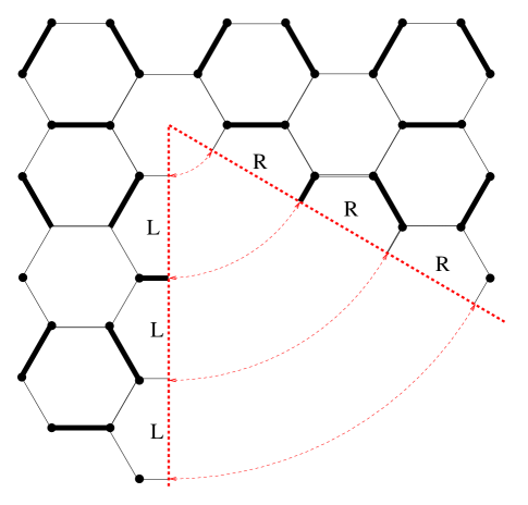
Figure 2: Cutting out a $60^{\circ}$ wedge and reconnecting the severed bonds leaves a pentagon disclination. When the apex of the wedge lies in a hexagon with no double bonds, single bonds reconnect to single bonds and double bonds to double bonds, leaving a globally consistent Fries-Kekulé structure.

We insert a pentagon disclination into the lattice by cutting out a $60^{\circ}$ wedge and rejoining the severed bonds. We wish to preserve the global Fries-Kekulé pattern, so the apex of the removed wedge must lie in a hexagon with no double bonds (see figure 2). In order for the lattice wavefunction to join smoothly across the seam of new bonds, the coefficient functions on the original lattice must obey the boundary conditions [9, 10]

$$\left(\matrix{f_{A+}\cr f_{B+}\cr f_{B-}\cr f_{A-}}\right)_{\rm R}=\left(\matrix{0&0&\bar{\eta}&0\cr 0&0&0&\eta\cr\bar{\eta}&0&0&0\cr 0&\eta&0&0}\right)\left(\matrix{f_{A+}\cr f_{B+}\cr f_{B-}\cr f_{A-}}\right)_{\rm L}.$$ (10)

Here the subscript R means the value to the right of the cut, and L to the left. In order to deal with this transformation it is convenient to change basis so that $\Psi=(f_{A+},f_{B+},f_{B-},-f_{A-})^{T}.$ This makes $\pm$ kinetic energy blocks become identical

$$H\left(\matrix{f_{A+}\cr f_{B+}\cr f_{B-}\cr-f_{A-}}\right)=\left(\matrix{0&-2\partial_{z}&\Phi&0\cr 2\partial_{{\bar{z}}}&0&0&-\Phi\cr\Phi&0&0&-2\partial_{z}\cr 0&-\Phi&+2\partial_{{\bar{z}}}&0}\right)\left(\matrix{f_{A+}\cr f_{B+}\cr f_{B-}\cr-f_{A-}}\right)$$ (11)

at the expense of complicating the mass terms. We can write the Hamiltonian matrix compactly as

$$H=({\mathbb{I}}\otimes\tilde{\mbox{\boldmath$\sigma$}})\cdot{\bf p}+\Phi\,\tau_{1}\otimes\sigma_{3},$$ (12)

where the $\mathbb{I}$ and $\tau_{1}$ matrices act on the two-by-two blocks (i.e. in the ${\bf K}$-${\bf K}^{\prime}$ space) and the $\sigma$ matrices act between the $A$ and $B$ sublattices within each ${\bf K}$, ${\bf K}^{\prime}$ block . (In the sequel we will omit $\mathbb{I}$ matrices when no ambiguity results.)

In the new basis, the operator $\Gamma$ that anti-commutes with $H$ remains

$$\Gamma=\tau_{3}\otimes\sigma_{3}\equiv\left(\matrix{\sigma_{3}&0\cr 0&-\sigma_{3}}\right).$$

The boundary condition, however, becomes

$$\left(\matrix{f_{A+}\cr f_{B+}\cr f_{B-}\cr-f_{A-}}\right)_{\rm R}=\left(\matrix{0&0&\bar{\eta}&0\cr 0&0&0&-\eta\cr\bar{\eta}&0&0&0\cr 0&-\eta&0&0}\right)\left(\matrix{f_{A+}\cr f_{B+}\cr f_{B-}\cr-f_{A-}}\right)_{\rm L}.$$ (13)

This can be factored as

$$\Psi_{\rm R} = -i\tau_{1}\otimes\exp\{-i\pi\sigma_{3}/6\}\Psi_{\rm L}$$ (14)

$$= \exp\{-i\pi\tau_{1}/2\}\otimes\exp\{-i\pi\sigma_{3}/6\}\Psi_{\rm L}.$$

As before, the $\tau_{1}$ matrix acts on the $\pm$ valley-degeneracy “flavour” indices and the $\sigma$ matrices on the $A,B$ “spin” indices.

Similarly, cutting out a 120^∘ wedge turns a hexagon into a square, and requires

$$\left(\matrix{f_{A+}\cr f_{B+}\cr f_{B-}\cr-f_{A-}}\right)_{\rm R}=\left(\matrix{\eta&0&0&0\cr 0&\bar{\eta}&0&0\cr 0&0&\eta&0\cr 0&0&0&\bar{\eta}}\right)\left(\matrix{f_{A+}\cr f_{B+}\cr f_{B-}\cr-f_{A-}}\right)_{\rm L}$$ (15)

which can be factored as

$$\Psi_{\rm R} = -{\mathbb{I}}\otimes\exp\{-i\pi\sigma_{3}/3\}\Psi_{\rm L}$$ (16)

$$= \exp\{-i\pi\tau_{1}\}\otimes\exp\{-i\pi\sigma_{3}/3\}\Psi_{\rm L}.$$

In this last line, the $\tau_{1}$ matrix in the exponent can be replaced by $\tau_{2}$, $\tau_{3}$, or even by $\mathbb{I}$, without altering the lattice boundary condition. The authors of [11] elected to take this matrix to be $\tau_{3}$ as this choice leads to a continuum hamiltonian for which the symmetry required by the Jackiw-Rossi-Weinberg index theorem appears manifest.

We can remove the discontinuity across the 60^∘ wedge by writing

$$\Psi(r,\theta)=\exp\left\{i{\pi\over 2}\tau_{1}\left({3\theta\over 5\pi}\right)\right\}\otimes\exp\left\{i{\pi\over 6}\sigma_{3}\left({3\theta\over 5\pi}\right)\right\}\tilde{\Psi}(r,\theta),$$ (17)

and across the 120^∘ wedge by writing

$$\Psi(r,\theta)=\exp\left\{i\pi\tau_{1}\left({3\theta\over 4\pi}\right)\right\}\otimes\exp\left\{i{\pi\over 3}\sigma_{3}\left({3\theta\over 4\pi}\right)\right\}\tilde{\Psi}(r,\theta).$$ (18)

Again, in the second case, we may replace the $\tau_{1}$ matrix by $\tau_{2}$, $\tau_{3}$ or ${\mathbb{I}}$. In all cases, the new field $\tilde{\Psi}(r,\theta)$ is continuous across the reconnected seam. In the first case the angle $\theta$ is restricted to the range $-\pi/6<\theta<3\pi/2$, with the limiting values representing the same point on the graphene cone, and in the second $\pi/6<\theta<3\pi/2$.

We wish to write the eigenvalue problem in polar coordinates whose origin is at the tip of the cone. To do this we use the identity

$$H = \tilde{\mbox{\boldmath$\sigma$}}\cdot{\bf p}+\Phi\,\tau_{1}\otimes\sigma_{3}$$ (19)

$$= -i\{\tilde{\sigma}_{1}\cos\theta+\tilde{\sigma}_{2}\sin\theta\}{\partial\over\partial r}-i\{-\tilde{\sigma}_{1}\sin\theta+\tilde{\sigma}_{2}\cos\theta\}{1\over r}{\partial\over\partial\theta}+\Phi\,\tau_{1}\otimes\sigma_{3}$$

$$= e^{-{i\over 2}\sigma_{3}\theta}\left(-i\tilde{\sigma}_{1}{\partial\over\partial r}-i\tilde{\sigma}_{2}{1\over r}\left({\partial\over\partial\theta}-{i\over 2}\sigma_{3}\right)+\Phi\,\tau_{1}\otimes\sigma_{3}\right)e^{{i\over 2}\sigma_{3}\theta}.$$

The coefficients of the derivatives $\sigma_{r,\theta}\equiv\tilde{\sigma}_{1,2}$ are now matrix-valued constants, but they pay for their constancy by being attached to a moving zweibein frame ${\bf e}_{r}$, ${\bf e}_{\theta}$. The $-i\sigma_{3}/2$ spin connection is therefore required to cancel the effect of taking the frame-rotation matrix $\exp\left\{i\sigma_{3}\theta/2\right\}$ through the $\theta$ derivative.

For planar graphene we would now define a new field $\chi(r,\theta)=e^{{i\over 2}\sigma_{3}\theta}\Psi(r,\theta)$ and find that it is antiperiodic under $\theta\to\theta+2\pi$. Because of the deleted wedge, however, we have to define

$$\chi(r,\theta)=\exp\left\{i\sigma_{3}\left({1\over 2}+{1\over 10}\right)\theta\right\}\tilde{\Psi}(r,\theta),$$ (20)

which is antiperiodic under $\theta\to\theta+2\pi\,(5/6)$. Taking into account eq. (17), the eigenvalue problem $H\Psi=E\Psi$ for the 60^∘ wedge can now be written

$$\left(-i\tilde{\sigma}_{1}{\partial\over\partial r}-i\tilde{\sigma}_{2}{1\over r}\left({\partial\over\partial\theta}-{i\over 2}\sigma_{3}+{3i\over 10}\tau_{1}\right)+\Phi\,\tau_{1}\sigma_{3}\right)\chi(r,\theta)=E\chi(r,\theta).$$ (21)

Here the $i\tau_{1}(3/10)$ gauge connection comes from taking the $\exp\left\{i\tau_{1}(3/10)\theta\right\}$ matrix appearing in equation (17) through the $\theta$ derivative. For the 120^∘ wedge we must set,

$$\chi(r,\theta)=\exp\left\{i\sigma_{3}\left({1\over 2}+{1\over 4}\right)\theta\right\}\tilde{\Psi}(r,\theta),$$ (22)

which is antiperiodic under $\theta\to\theta+2\pi\,(2/3)$. The corresponding eignevalue problem becomes

$$\left(-i\tilde{\sigma}_{1}{\partial\over\partial r}-i\tilde{\sigma}_{2}{1\over r}\left({\partial\over\partial\theta}-{i\over 2}\sigma_{3}+{3i\over 4}\tau_{1}\right)+\Phi\,\tau_{1}\sigma_{3}\right)\chi(r,\theta)=E\chi(r,\theta).$$ (23)

From now on, for purely cosmetic reasons, we will make the rotation introduced in (6) that removes the tildes from the $\sigma_{1,2}$ matrices. This does not affect the gauge fields, as they act in the valley degeneracy “flavour” space and the redefinition acts in the A-B “spin” space.

We define a new angle $\phi=(6/5)\theta$, or $\phi=(3/2)\theta$ that has the usual $2\pi$ periodicity. ($\phi$ is the polar angle seen when looking along the axis of the 60^∘ or 120^∘ cones from above their apex.) Using $\phi$ we can then separate the radial and angular part of the wavefunction as

$$\chi(r,\phi)=e^{ij\phi}\chi(r)$$ (24)

where $j$ takes half-integer values

$$j=\ldots,-{3\over 2},-{1\over 2},+{1\over 2},+{3\over 2}\ldots.$$ (25)

Note that the hermiticity of the radial part of the differential operator with respect to the inner product

$${\langle\Psi_{1}|\Psi_{2}\rangle}\stackrel{{\scriptstyle\rm def}}{{=}}\int_{0}^{2\pi}\!\!\!\!\int_{0}^{\infty}\Psi^{\dagger}_{1}\Psi_{2}\,rdrd\phi$$ (26)

requires a contribution from the spin-connection term $-i\sigma_{3}/2$ that occurs in the angular covariant derivative part:

$$-i\sigma_{2}{1\over r}\left({\partial\over\partial\theta}-{i\over 2}\sigma_{3}\right)=-i\sigma_{2}{1\over r}{\partial\over\partial\theta}-{i\over 2r}\sigma_{1}.$$ (27)

The $i\sigma_{1}/2r$ ensures that

$$\left(-i\sigma_{1}{\partial\over\partial r}-{i\over 2}\sigma_{1}\right)^{\dagger} = -i\sigma_{1}{1\over r}{\partial\over\partial r}r+{i\over 2}\sigma_{1}$$ (28)

$$= -i\sigma_{1}{\partial\over\partial r}-{i\over 2}\sigma_{1}.$$

Because $\tau_{1}$ commutes with $H$, we can find solutions to (21) and (23) (without the tilde’s) of the form

$$\chi_{+}(r,\phi)=\left(\matrix{u(r)\cr v(r)\cr u(r)\cr v(r)}\right)e^{ij\phi},\quad\chi_{-}(r,\phi)=\left(\matrix{u(r)\cr v(v)\cr-u(r)\cr-v(r)}\right)e^{ij\phi},$$ (29)

which are eigenvectors of $\tau_{1}$ with eigenvalue $\pm 1$. The functions $u(r),v(r)$ then satisfy

$$-i\left({d\over dr}+{1\over 2r}+{1\over r}{(j\pm n/4)\over 1-n/6)}\right)v+\tau\Phi u = Eu,$$

$$-i\left({d\over dr}+{1\over 2r}-{1\over r}{(j\pm n/4)\over 1-n/6)}\right)u-\tau\Phi v = Ev.$$ (30)

Here $n=1$ for the 60^∘ cone and $n=2$ for the 120^∘ cone. The number $\tau=\pm 1$ denotes the eigenvalue of $\tau_{1}$. Set

$$\nu={j+\tau n/4\over 1-n/6}.$$ (31)

We have continuous-spectrum eigenfunctions with $u,v$ of the form

$$\left(\matrix{u(r)\cr v(r)}\right) = \left(\matrix{(\epsilon+\tau\Phi)J_{\nu-1/2}(kr)\cr ikJ_{\nu+1/2}(kr)}\right),\quad E=\epsilon\equiv+\sqrt{k^{2}+\Phi^{2}},$$

$$\left(\matrix{u(r)\cr v(r)}\right) = \left(\matrix{ikJ_{\nu-1/2}(kr)\cr(\epsilon+\tau\Phi)J_{\nu+1/2}(kr)}\right),\quad E=-\epsilon,$$ (32)

and also

$$\left(\matrix{u(r)\cr v(r)}\right) = \left(\matrix{(\epsilon+\tau\Phi)J_{-(\nu-1/2)}(kr)\cr-ikJ_{-(\nu+1/2)}(kr)}\right),\quad E=\epsilon\equiv+\sqrt{k^{2}+\Phi^{2}},$$

$$\left(\matrix{u(r)\cr v(r)}\right) = \left(\matrix{-ikJ_{-(\nu-1/2)}(kr)\cr(\epsilon+\tau\Phi)J_{-(\nu+1/2)}(kr)}\right),\quad E=-\epsilon.$$ (33)

The first set of solutions is finite at the origin when $j>1/2$ and the second is finite at the origin when $j<-1/2$. For $j=1/2$ and $\tau$ negative, the upper component of the first set of solutions diverges at the origin, but no faster than $r^{-1/2}$, so it is normalizable there. Similarly the second set is locally normalizable for $j=-1/2$.

For most values of $j$ and $\tau$, demanding nomalizability is sufficient to select the physically allowed solutions. When $n=2$, however, and for $j=1/2$, $\tau=-1$, we have $\nu=0$. We also have $\nu=0$ when $j=-1/2$, $\tau=+1$. In these cases, the eigenvalue equation becomes

$$-i\left({d\over dr}+{1\over 2r}\right)v+\Phi\tau u = Eu$$

$$-i\left({d\over dr}+{1\over 2r}\right)u-\Phi\tau v = Ev.$$ (34)

The scattering solutions with $E=\pm\sqrt{k^{2}+\Phi^{2}}$ contain the Bessel function $J_{1/2}(kr)=\sqrt{2\pi/kr}\sin kr$ and $J_{-1/2}(kr)=\sqrt{2\pi/kr}\cos kr$, both of which are normalizable near the singular point at the origin. The equation is therefore in Weyl’s limit-circle class there, and some additional boundary condition must be imposed to select a complete, linearly independent, set of solutions [19].

One reason for the $n=2$, 120^∘ wedge differing from the $n=1$, 60^∘ wedge is that that the cutting and sewing of the graphene sheet in the former case preserves the A-B bipartite structure of the lattice. There should therefore be a some operator that anti-commutes with the Hamiltonian. This property is not easy to see in eq (23), but becomes clearer if we elect to replace the gauge field term with $\tau_{3}$. Then equation (18) defining the single-valued field $\tilde{\Psi}(r,\theta)$ becomes

$$\Psi(r,\theta)=\exp\left\{i\pi\tau_{3}\left({3\theta\over 4\pi}\right)\right\}\otimes\exp\left\{i{\pi\over 3}\sigma_{3}\left({3\theta\over 4\pi}\right)\right\}\tilde{\Psi}(r,\theta),$$ (35)

and the eigenvalue equation (23) is replaced by

$$\left(-i\sigma_{1}\left({\partial\over\partial r}+{1\over 2r}\right)-i\sigma_{2}{1\over r}\left({3\over 2}{\partial\over\partial\phi}+{3i\over 4}\tau_{3}\right)+\Phi\,\sigma_{3}(\tau_{1}\cos\phi+\tau_{2}\sin\phi)\right)\chi(r,\theta)=E\chi(r,\theta),$$ (36)

with antiperiodic $\chi(r,\theta)$. This is the equation with a unit-winding-number vortex in the mass term that was considered in [11]. It is formally of the form to which the Jackiw-Rossi-Weinberg index theorem applies: the matrix-valued differential operator manifestly anti-commutes with $\Gamma=\tau_{3}\otimes\sigma_{3}$, and the index is the Hilbert-space trace of $\Gamma$.

Eq (36) posseses zero energy solutions of the form

$$\chi(r,\phi)=\left(\matrix{e^{-i\phi/2}u(r)\cr 0\cr 0\cr e^{i\phi/2}v(r)}\right),\quad\chi(r,\phi)=\left(\matrix{0\cr e^{-i\phi/2}v(r)\cr e^{i\phi/2}u(r)\cr 0}\right),$$ (37)

which are eigenvectors of $\Gamma$ with eigenvalues $+1$ and $-1$ respectively. Ignoring any constraints imposed by boundary conditions they are

$$\Psi_{0+-}=\left(\matrix{e^{-i\phi/2}\cr 0\cr 0\cr ie^{i\phi/2}}\right){1\over\sqrt{r}}e^{-\Phi r},\quad\Psi_{0--}=\left(\matrix{0\cr ie^{-i\phi/2}\cr e^{i\phi/2}\cr 0}\right){1\over\sqrt{r}}e^{-\Phi r},$$ (38)

and

$$\Psi_{0++}=\left(\matrix{ie^{-i\phi/2}\cr 0\cr 0\cr e^{i\phi/2}}\right){1\over\sqrt{r}}e^{+\Phi r},\quad\Psi_{0-+}=\left(\matrix{0\cr e^{-i\phi/2}\cr ie^{i\phi/2}\cr 0}\right){1\over\sqrt{r}}e^{+\Phi r},$$ (39)

Only one pair will be normalizable, depending on the sign of $\Phi$.

Eq (36) also posses more general bound-state solutions for any value of $E$ in the range $-|\Phi|<E<|\Phi|$. These are

$$\Psi_{E,1}=\left(\matrix{(E+\Phi)e^{i\phi/2}\cr i\kappa e^{i\phi_{2}}&\cr(E+\Phi)e^{-i\phi/2}\cr i\kappa e^{-i\phi}}\right){1\over\sqrt{r}}e^{-\kappa r},\quad\Psi_{E,2}=\left(\matrix{(E-\Phi)e^{i\phi}\cr i\kappa e^{i\phi/2}\cr(\Phi-E)e^{-i\phi/2}\cr-i\kappa e^{-i\phi/2}}\right){1\over\sqrt{r}}e^{-\kappa r}$$ (40)

and

$$\Psi_{E,3}=\left(\matrix{(E+\Phi)e^{i\phi/2}\cr-i\kappa e^{i\phi/2}\cr(E+\Phi)e^{-i\phi/2}\cr-i\kappa e^{-\phi/2}}\right){1\over\sqrt{r}}e^{+\kappa r},\quad\Psi_{E,4}=\left(\matrix{(E-\Phi)e^{i\phi/2}\cr-i\kappa e^{i\phi/2}\cr(\Phi-E)e^{-i\phi/2}\cr i\kappa e^{-i\phi/2}}\right){1\over\sqrt{r}}e^{+\kappa r}.$$ (41)

Here $\kappa=\sqrt{\Phi^{2}-E^{2}}$. These solutions are not eigenfunctions of $\Gamma$. Instead $\Gamma$ acts on them to give a solution with energy $-E$.

Both the $E=0$ and the more general $-|\Phi|<E<|\Phi|$ solutions are square integrable in the neighbourhood of $r=0$. The same is true of the scattering state solutions with $|E|>|\Phi|$. We need to impose some boundary condition at $r=0$ to select from these solutions a complete linearly-independent set. As a guide to the form of this boundary condition we apply the Weyl-von-Neumann theory [20]. The matrix-valued differential operator determining the radial part of all these solutions is

$$H=-i\sigma_{1}\left({d\over dr}+{1\over 2r}\right)+\Phi\,\tau_{1}\otimes\sigma_{3},\quad r\in[0,\infty).$$ (42)

If we restrict it an initial domain that contains only functions that vanish at $r=0$, the resulting linear operator has deficiency indices $(2,2)$. The restricted operator therefore admits a four-parameter family of self-adjoint extensions. To determine the corresponding boundary conditions, we evaluate ${\langle\Psi|HX\rangle}-{\langle H\Psi|X\rangle}$ on functions $\Psi=(\psi_{1},\psi_{2},\psi_{3},\psi_{4})^{T}$ and $X=(\chi_{1},\chi_{2},\chi_{3},\chi_{4})^{T}$ that are square integrable on $[0,\infty)$ with the measure $r\,dr$. We find that

$${\langle\Psi|HX\rangle}-{\langle H\Psi|X\rangle}=[-ir(\psi_{1}^{*}\chi_{2}+\psi_{2}^{*}\chi_{1}+\psi_{3}^{*}\chi_{4}+\psi_{4}^{*}\chi_{3})]_{0}^{\infty}.$$ (43)

Since $\Psi(r)$ and $X(r)$ are allowed to diverge as $r^{-1/2}$ near the origin but must tend to zero faster than $r^{-2}$ at infinity, the vanishing of the integrated-out part requires that the expression in parentheses tend to zero at $r=0$. If we impose boundary conditions

$$\left(\matrix{\psi_{1}\cr\psi_{3}}\right)=\left(\matrix{a&b\cr c&d}\right)\left(\matrix{\psi_{2}\cr\psi_{4}}\right),\quad r\to 0$$ (44)

on $\Psi(r)$, the adjoint boundary conditions on $X(r)$ are determined by requiring that

$$\lim_{r\to 0}[\psi_{2}^{*}(a^{*}\chi_{2}+c^{*}\chi_{4}+\chi_{1})+\psi_{4}^{*}(b^{*}\chi_{2}+\chi_{3}+d^{*}\chi_{4})]=0$$ (45)

for any $\psi_{2}$, $\psi_{4}$. Thus the adjoint boundary conditions are

$$\left(\matrix{\chi_{1}\cr\chi_{3}}\right)=\left(\matrix{-a^{*}&-c^{*}\cr-b^{*}&-d^{*}}\right)\left(\matrix{\chi_{2}\cr\chi_{4}}\right),\quad r\to 0.$$ (46)

For $H$ to be self-adjoint, these boundary conditions must coincide with the boundary conditions imposed on $\psi$. We there have that, as $r\to 0$,

$$\left(\matrix{\psi_{1}\cr\psi_{3}}\right)=\left(\matrix{iA&B+iC\cr-B+iC&iD}\right)\left(\matrix{\psi_{2}\cr\psi_{4}}\right).$$ (47)

for real (possiby infinite) numbers $A$, $B$, $C$ and $D$. This relation contains the four real parameters required by the Weyl-von Neumann count, and so is the most general possible self-adjoint boundary condition.

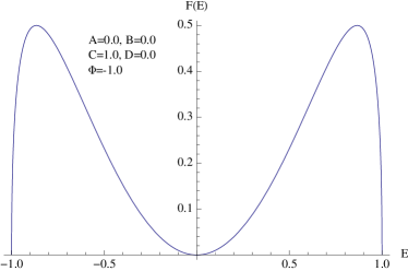
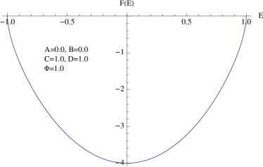
Figure 3: The left-hand plot shows $F(E)$ for boundary-condition parameters $A=B=D=0$, $C=1$, and $\Phi=-1$ which possesses two degenerate zero modes. The right-hand plot shows $F(E)$ for the same boundary parameters, but with $\Phi$ having changed sign from negative (reduced hopping in the double bonds) to positive (enhanced hopping on the double bonds). There are now no bound states.

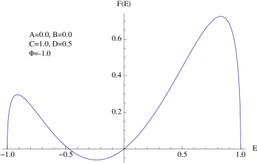
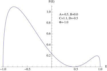
Figure 4: The left-hand figure shows $F(E)$ for $A=B=0$, $C=1$, $D=.5$ and $\Phi$ negative. There is a zero mode and a bound state with $E\approx-0.5|\Phi|$. In the right-hand figure we have $A=D=-1.0$, $B=0$, $D=\sqrt{2}$, and $\Phi$ negative. There are two degenerate bound states at $E=|\Phi|/\sqrt{2}$. In both cases, the bound states cease to exist as soon as $\Phi$ changes sign from negative to positive.

The numerical solution of the 120^∘ wedge-cut lattice show that there are two exact zero modes that are localized when $\Phi<0$ and become delocalized when $\Phi>0$. These modes can be identified with $\Psi_{0++}$ and $\Psi_{0-+}$, and are allowed if we impose the boundary condition

$$\left(\matrix{\psi_{1}\cr\psi_{3}}\right)=\left(\matrix{0&i\cr i&0}\right)\left(\matrix{\psi_{2}\cr\psi_{4}}\right)$$ (48)

at $r=0$. The other potential zero modes $\Psi_{0+-}$ and $\Psi_{0--}$ do not satisfy this condition.

For general values of $A$, $B$, $C$ and $D$, we can seek bound-state solutions of the form

$$\Psi=\alpha\Psi_{E,1}+\beta\Psi_{E,2}.$$

Imposing the boundary condition (47) at $r=0$ leads to a pair of homogeneous equations

$$(\alpha+\beta)E+(\alpha-\beta)\Phi = -A\kappa(\alpha+\beta)-(C-iB)\kappa(\alpha-\beta),$$

$$(\alpha-\beta)E+(\alpha+\beta)\Phi = -D\kappa(\alpha-\beta)-(C+iB)\kappa(\alpha+\beta),$$ (49)

for $\alpha$ and $\beta$, and hence to the condition $F(E)=0$, where

$$F(E)=\left|\matrix{E+A\kappa&\Phi+(C-iB)\kappa\cr\Phi+(C+iB)\kappa&E+D\kappa}\right|.$$ (50)

The function $F(E)$ is real in the range $-|\Phi|\leq E\leq|\Phi|$, and always has two zeros at $E=\pm|\Phi|$ corresponding to the edges of the upper and lower continuum respectively. Additional zeros in the range $-|\Phi|<E<|\Phi|$ correspond to the energies of bound states. Example plots of $F(E)$ for different values of $A$, $C$, $D$ and $\Phi$ are shown in figures 3 and 4. Of particular interest is the left hand plot in figure 3 which exhibits the pair of $E=0$ zero modes for the boundary conditions in (48), and the right-hand plot in figure 4 which exhibits a pair of degenerate levels at a non-zero value of $E$. The plots in figure 4 correspond to non-zero values for one or both of the parameters $A$ and $D$. These parameters control the boundary coupling of the A and B lattices to themselves, and non-zero values violate the bipartite lattice structure that leads to the $E\leftrightarrow-E$ spectral symmetry possessed by the bulk differential equation.

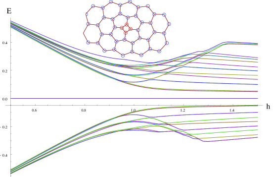
Figure 5: The low-lying part of the energy spectrum plotted versus $h$ (the ratio of double bond hopping to single bond hopping) for a square defect created by excising a 120^∘ wedge. The horizontal axis has been displaced vertically so as to uncover the doubly-degenerate exact zero mode. The “within-gap” modes peeling off from the upper and lower continua for $h>1$ (i.e. $\Phi>0$) are “anti-localized” edge states, whose exact form depends on how we truncate the lattice on its outer boundary.

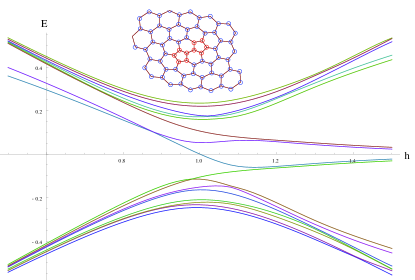
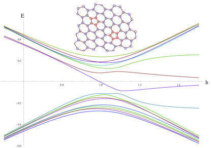
Figure 6: The low-lying energy spectrum plotted versus $h$ for a pair of nearby pentagons. The left-hand figure is for an $(n.m)=(1,1)$ cone in the languge of ref [9], and the right-hand figure is for an $(n,m)=(0,3)$ cone. In both cases the 60^∘ wedges have their apices in single-bond hexagons so as to preserve the global Kekulé structure. For $h<1$ there is a pair of nearly degenerate bound states lying just below the upper continuum. The “below gap” modes at $h>1$ are uninteresting edge states localized at the outer boundary.

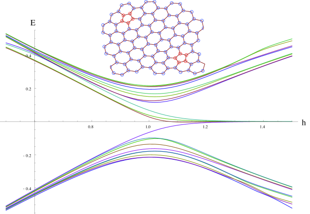
Figure 7: The low-lying energy spectrum plotted versus $h$ for a pair of pentagons forming a $(n,m)=(0,6)$ cone.

Figures 5, 6 and 7 show some numerical plots of the low-lying energy states as a function of $h=(t+\delta t)/t$, where $\delta t$ is the change in hopping parameter on the double bonds (recall that $\Phi=(2/3at)\delta t$.). In all four lattices, the wedges have their apices in single-bond hexagons, so that the global Kekulé structure is preserved. In the language of [9] they all have $n=m\,\hbox{\rm mod\,}3$, ensuring that the asymptotic gauge field is the same in all four cases. The spectra differ, however, because the boundary conditions seen by the continuum wave functions at the tip of the cone are different. In the case of figure 5, the global bipartite structure is preserved, the boundary conditions are those of eq. (48) and so the spectrum is manifestly $E\leftrightarrow-E$ symmetric. In lattices of figures 6 and 7 the bipartite structure is scrambled in the region between the pentagons and so the $E\leftrightarrow-E$ symmetry is violated. All of the two-pentagon cases display a pair of almost degenerate bound states just below the positive continuum, and are therefore similar to the spectrum associated with the boundary conditions of the right-hand plot of figure 4. As $h$ approaches unity, and $\Phi$ approaches zero, the wave functions begin to spread out and see the outer boundary of our large-but-finite lattices (2644 vertices in case of the square and 1158 vertices for the pair of pentagons). The effects of this can be seen in the figures in the splitting of the bound-state energies as $h$ approaches unity from below.

IV Conclusions

The continuum Dirac hamiltonian provides a good account of the low-energy, long-wavelength, eigenstates of the tight-binding hamiltonian on an infinite sheet of graphene. The continuum model is also a useful approximation for cones tipped by curvature singularities induced by pentagon defects — but it must be supplemented by non-trivial boundary conditions at the tip of the cone. Although the low-lying eigenfunctions have too long a wavelength to resolve the fine details of lattice disruption at the tip, they there experience phase shifts and mode mixing that have a significant effect on the eigenstates. For two separated pentagons, the scrambling of the A-B bipartite lattice structure along a seam joining the pentagons sufficiently violates the $E\leftrightarrow-E$ spectral symmetry as to allow bound states at non-zero $E$. In the case of two coincident pentagons (i.e. a square) the $E\leftrightarrow-E$ symmetry is preserved, but (in contrast to the quarter-unit flux through a pentagon) the resultant half-unit of flux through the square plaquette is too large to be approximated by a spread-out gauge field. A continuum gauge field with this flux would have bound a single state whose eigenvalue of $\Gamma$ is determined by the sign of the flux. The lattice spectrum must be unchanged, however, by the insertion of an integer flux-quantum through the square. Such an insertion can reverse the sign of the flux and so no particular sign of $\Gamma$ can be favoured. The lattice hamiltonian compromises by producing two bound states, one with each sign of $\Gamma$. All these effects can be reproduced in the continuum model by suitable choices of the parameters in the self-adjoint boundary conditions. However, the predictions [11] of the continuum Jackiw-Rossi-Weinberg theorem do not survive in a simple form. It will be interesting to see if the theorem can be modified to include the effects of the singular endpoint.

V Acknowledgements

This work was supported by the National Science Foundadation under grant DMR-06-03528. Some of the work was carried at the KITP in Santa Barbara, and so supported in part by the National Science Foundation under grant PHY05-51164. We would like to thank Jiannis Pachos for many discussions, and Jeremy Oon for his assistance with the numerical work at the beginning of this project.

References

- [1] A. K. Geim and K.S. Novoselov, Nature Materials 6, 183-191 (2007).
- [2] P. R. Wallace, Phys. Rev. 71 622-634 (1949).
- [3] K. Fries, Justus Liebigs Annalen der Chemie 454 121-324 (1927); K. Fries, R. Walter, K. Schilling, Justus Liebigs Annalen der Chemie 516 248-285 (1935).
- [4] E. Clar, The Aromatic Sextet, John Wiley & Sons, New York (1972).
- [5] C.-Y. Hou, C. Chamon, and C. Mudry, Phys. Rev. Lett. 98, 186809 (2007).
- [6] C. Chamon, C.-Y. Hou, R. Jackiw, C. Mudry, S.-Y. Pi, G. Semenoff. Phys. Rev. B77 235431 (2008).
- [7] P. Ghaemi and F. Wilczek, arXiv:07092626 (2007).
- [8] P. Ghaemi, S. Ryu, D-H. Lee, arXiv:0903.1662 (2009).
- [9] P. E. Lammert, and V. H. Crespi, Phys. Rev. Lett. 85, 5190 (2000); Phys. Rev. B 69, 035406 (2004).
- [10] D. V. Kolesnikov and V. A. Osipov, Eur. Phys. J. B 49, 465 (2006); V. A. Osipov, E. A. Kochetov, JEPT 73, 631 (2001).
- [11] J. Pachos, M. Stone, K, Temme, Phys. Rev. Lett. 100 156806 (2008).
- [12] J K. Pachos, Contempory Phys. 50, 375 (2009).
- [13] J. Gonzalez, F. Guinea, M. A. H.Vozmediano, Phys. Rev. Lett. 69 172-175 (1992).
- [14] J. Gonzalez, F. Guinea, M. A. H.Vozmediano, Nucl. Phs. B406 [FS5] 771-794 (1993).
- [15] R. Jackiw , P. Rossi, Nucl. Phys. B 190, 681 (1981).
- [16] E. Weinberg, Phys. Rev. D 24 2669 (1981).
- [17] P. W. Fowler, M. Fujita, M. Yoshida, J. Chem. Soc. Faraday Trans. 92 3763-3675 (1996).
- [18] K. M. Rogers, P. W. Fowler, J. Chem. Soc. Perkin Trans. 2 18-22 (2001).
- [19] H. Yamagishi, Phys. Rev. D27 2383 (1983).
- [20] See for example: R. D. Richtmyer Principles of Advanced Mathematical Physics (Springer Verlag 1978) Vol I, §8.6.