Hidden Noise Structure and Random Matrix Models of Stock Correlations

Abstract

We find a novel correlation structure in the residual noise of stock market returns that is remarkably linked to the composition and stability of the top few significant factors driving the returns, and moreover indicates that the noise band is composed of multiple subbands that do not fully mix. Our findings allow us to construct effective generalized random matrix theory market models LalouxEtal00_RMT ; PlerouEtal_PRE02 that are closely related to correlation and eigenvector clustering Mantegna_HierarchicalClust ; GopiEtal_ClustSectors . We show how to use these models in a simulation that incorporates heavy tails. Finally, we demonstrate how a subtle purely stationary risk estimation bias can arise in the conventional cleaning prescription LalouxEtal00_RMT .

Introduction:

Originally started in the context of nuclear physics Mehta_RMTbook , random matrix theory (RMT) has thereafter found numerous applications in a variety of fields such as number theory, disordered systems, neural networks, and signal processing Mehta_RMTbook ; SenguptaMitra99 . Recently the pioneering work of Laloux et al LalouxEtal00_RMT , as well as much subsequent research PlerouEtal_PRE02 ; RMT_other , have shown that RMT can also be a valuable tool for analyzing stock market correlations, where noise can account for more than 2/3 of the eigenvalue spectrum, and a typical large portfolio has size comparable to the measurement time frame. Thus, much of the empirical eigenvalues are spurious and represent measurement noise and biases. The remarkable insight provided by Laloux et al was to show that a suitable fit to RMT can clean these spurious contributions, and moreover identify the statistically significant signal, or common market risk factors that drive the individual stock returns. The most prominent such non-idiosyncratic factor is the nearly equal-weight top eigenvector, whose eigenvalue is more than 20 times bigger than the average spectrum. Secondary factors, are long-short portfolios of certain liquidity LalouxEtal00_RMT and industry structure GopiEtal_ClustSectors ; AvellanedaLee_StatArb , but their contribution is typically an order of magnitude smaller. Most of the rest of the eigenvectors are unstable in time, appear random, and their spectral contribution can be fitted to the Marcenko-Pasteur (MP) distribution MarcenkoPasteur derived in the context of Gaussian RMT (GRMT). The noisy eigenvalue correlations PlerouEtal_PRE02 also agree with theory Mehta_RMTbook . These results have been verified over many stock selections, as well as return frequencies LalouxEtal00_RMT ; PlerouEtal_PRE02 ; RMT_other .

Despite the apparent success of the theory, subsequent research suggests several empirical aspects that the original RMT cleaning may not account for properly. (1) Tails and their correlations have non-trivial effects, and are known to both broaden the spectrum above the upper noise-band edge, as well sharpen it near the lower edge PlerouEtal_PRE02 ; BouchaudEtal_FatTailsRMT ; RMT_fatTailsOther , thus making the fit to the MP distribution problematic. The above redistribution of spectral weight appears in conjunction with an enhancement of the inverse participation ratios around both ends of the noise spectrum, the so-called localization effect PlerouEtal_PRE02 , unlike GRMT where the participations are flat Mehta_RMTbook . (2) In addition to being partially localized, the band itself may be split due to the same separation of correlation scales LilloMantegna that is thought to give rise to clustering of stocks between industries Mantegna_HierarchicalClust . So far this effect has not been observed, however, due to the large amount of mixing that depletes the stability of all the noisy eigenvectors. It is important to empirically distinguish between the single and multiple band cases. (3) Non-stationarity effects are insufficiently understood. They are suggested LalouxEtal00_RMT ; PlerouEtal_PRE02 to be the source of a residual bias in the risk estimates obtained after RMT cleaning. However, in light of the abovementioned considerations, it is not clear that the original cleaning procedures are unbiased to begin with.

In this work, we consider both $N=484$ $2$ minute S&P500 TAQ midquote returns between June 20 - Sep 20, 2007, as well as $N=451$ daily S&P500 returns between Jan 2001-Dec 2007 Foot_AutocorrRemoval . (1) We reveal a novel correlation structure of the residuals that is linked to the structure and stability of the top few empirical factors. Mainly, we find that the inverse participations of the localized edge-eigenmodes of the band are dominated by the outlier stocks in the composition of the top few factors, thus indicating that most of the noise there is due to these stocks. The upper edge fluctuations are mainly due to weakly correlated stocks with the smallest relative weight in the market portfolio while lower edge fluctuations are due to strongly correlated stocks identified as the outliers in the secondary factors. The groups in the lower edge belong to major industrial sectors PlerouEtal_PRE02 ; Mantegna_HierarchicalClust , while the upper edge contains a large diversified portfolio of medium to small liquidity stocks. Moreover, because we find these groups to be disjoint, we conclude that as long as the top few factors are stable and distinct, the noise band is composed of multiple subbands that do not fully mix. (2) We pinpoint the effective positive-definite cleaned matrices that exhibit the multi-residual and factor structure above to be the hierarchical RMT models LilloMantegna , which are closely related to coarse-grained “real space” models of market clustering Mantegna_HierarchicalClust , and fundamentally arise out of correlation scale separation. (3) We use these effective models to perform a one-factor stochastic volatility BouchaudEtal_FatTailsRMT simulation in order to take into account the effect of tails and their correlations. (4) We show how conventional cleaning can give rise to a subtle purely stationary risk-estimation bias.

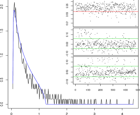
Figure 1: Main: A fit of the MP distribution to $2$ min data for $N=484,$ stocks in the S&P 500 with $T=3N$ yields $Q_{eff}=2.25$, and $\sigma_{eff}=0.67$. The top three eigenvalues, $\lambda_{1}=152.9$, $\lambda_{2}=8.2$, $\lambda_{3}=7.6$, $\lambda_{4}=5.3$, $\lambda_{5}=5.2$ were omitted from the plot due to their scale. Inset: The top three eigenvectors, $e_{ki},$ $k=1,2,3$, with their entries $i$ sorted by decreasing liquidity (from left to right). Note the significant outliers in each $e_{k}$ as emphasized by the horizontal lines.

Empirical Results:

Given our set of $N$ stock series $S_{i}(t)$, $t=1,\ldots,T$, from their log returns $x_{t,i}=\log(S_{t,i}/S_{t-1,i})$ we calculate the empirical correlation $C_{E}=(\langle x_{i}x_{j}\rangle-\langle x_{i}\rangle\langle x_{j}\rangle)/\sigma_{i}\sigma_{j}$ where $\sigma_{i}=\sqrt{\langle x_{i}^{2}\rangle-\langle x_{i}\rangle^{2}}$. According to RMT Mehta_RMTbook ; SenguptaMitra99 ; LalouxEtal00_RMT , if $C_{E}$ were obtained from a purely random signal of bounded variance $\sigma$ whose marginal tails are not too heavy BouchaudEtal_FatTailsRMT , then in the limit $N\rightarrow\infty$ with $Q\equiv N/T$ fixed, the correlations will self-average and will have an asymptotically deterministic eigenvalue spectrum given by the MP distribution MarcenkoPasteur :

$$p_{MP}(\lambda)=\frac{Q}{2\pi\sigma^{2}}\frac{\sqrt{(\lambda_{+}-\lambda)(\lambda-\lambda_{-})}}{\lambda}.$$ (1)

In the above, the eigenvalues $\lambda$ are restricted to lie within the hard-edge spectral band, $\lambda\in[\lambda_{-},\lambda_{+}],$ with $\lambda_{\pm}=\lambda_{\pm}(Q,\sigma)=\sigma^{2}(1\pm\sqrt{1/Q})^{2}$. One can interpret (1) as the the finite $T/N$ noise-induced broadening and bias away from the underlying trivial spectrum $p_{clean}(\lambda)=\delta(\lambda-1)$ that $p_{MP}(\lambda)$ reduces to in the limit $Q\rightarrow\infty$.

Of course, stock market correlations are not purely random, so a fit for $\sigma$ and $Q$ is necessary in (3) if one wants to identify the trully residual part of the spectrum LalouxEtal00_RMT ; PlerouEtal_PRE02 . In Fig. 1 we show such a fit to the noisy region of the $2$ min data that yields $\sigma_{eff}=0.67,$ $Q_{eff}=2.25.$ Note that much of the spectrum lies outside the MP band. In the inset of Fig 1 we plot the composition, of the top three eigenvectors $\{e_{k}\}$, $k=1,2,3$ sorted by decreasing liquidity. Unlike the prediction of GRMT where $e_{k}$ should be a mean-zero unit Gaussian, there are clear deviations from such behavior in all three eigenvectors, as emphasized in the inset. In fact, $e_{1}$ has non-zero mean, $\langle e_{1i}\rangle_{i}=0.044\simeq N^{-1/2}$, representing a long-only market portfolio, while $e_{2}$ and $e_{3}$ represent long-short portfolios. All three $e_{k}$ can be interpreted as significant common factors. Furthermore, as is clear from the plot, the outliers in the factor composition have certain liquidity structure. In the case of $e_{2}$ and $e_{3}$ in of Fig 1, these outliers can be identified with major sectors such as financials, oil, and utilities, whose correlations are relatively stable in time GopiEtal_ClustSectors ; AvellanedaLee_StatArb ; Mantegna_HierarchicalClust .

Despite the appearance of factors, one expects the random residual spectral contribution to be well fitted to RMT. However, there are important issues with the fit to $p_{MP}$ that one needs to address. Heavy tails in the multivariate distribution of $x_{t,i}$ have non-trivial effects. They are known to broaden the spectral weight above the upper edge, as well as sharpen it near the lower edge PlerouEtal_PRE02 ; BouchaudEtal_FatTailsRMT ; RMT_fatTailsOther , both features readily noticeable in Fig. 1 as well as in daily data LalouxEtal00_RMT . Moreover, such tails tend to induce outliers in the composition of the principal components near the band edge BouchaudEtal_FatTailsRMT causing deviations from the standard Gaussian distribution of the composition expected by GRMT and inducing localization. Indeed, just as in daily data PlerouEtal_PRE02 we see in the $2$ min returns that the eigenvectors are localized at both ends of the noise spectrum by computing the inverse participation ratio PlerouEtal_PRE02 , $I_{k}=\sum_{i=1}^{N}[e_{ki}]^{4}$ for each eigenvector $e_{k}$. Intuitively, the participation $P_{k}\equiv 1/I_{k}$ scales as the number of non-trivial entries in a normalized $e_{k}$: $P_{k}=N$ for equal weight vectors, while $P_{k}=1$ for a single non-trivial weight. As evident in Fig 2 (a), the participation is strongly localized near the band edges indicating that the eigenvectors there are dominated by outliers.

A nice trick that avoids estimating the effects of tails is to clean the noisy eigenvalues $\Lambda_{E}=diag(\lambda_{1},\ldots,\lambda_{K};\{\lambda_{noise}\})$ of $C_{E}=S_{E}\Lambda_{E}S_{E}^{\prime}$ with a flat band with scale proportional to $\sigma_{eff}$ while working in the original eigenvector basis $S_{E}=(e_{1},\ldots,e_{N})$ LalouxEtal00_RMT , thus obtaining a “filtered” matrix PlerouEtal_PRE02 . In fact, unless the empirically measured tail fluctuations significantly break the rotational invariance implied by cleaning with a flat band, $\sigma_{eff}$ can be thought of as the overall scale of the residual noise that one can tune even without fitting to the Gaussian formula. The feasibility of this “filtering” procedure can also be justified with the resulting significant improvement of the portfolio risk estimates that one obtains with cleaning LalouxEtal00_RMT ; GopiEtal_ClustSectors .

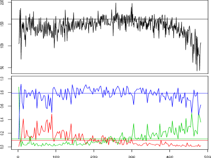
Figure 2: Top: The participation $P_{k}$ of the eigenvectors $e_{k}$, $k\geq 2$ for the data in Fig 1 exhibits localization. Flat horizontal line represents $P_{k}^{GMRT}=N/3.$ Mehta_RMTbook . Bottom: Relative inverse participation $R_{k}^{(G)}$ for the groups $G_{1}$ (red), $G_{23}$ (green) and $G^{\perp}$ (blue) defined in the text. Flat lines represent $R_{k,RMT}^{(G)}$.

We will now show, however, that because of a novel structure of the eigenvectors, cleaning with a flat band $\sigma_{eff}$ is inconsistent with their symmetry. Suppose we look at the following group of stocks, $\{G_{1},G_{k}^{\pm},G^{\perp}\},$ $k=2,3$ selected so that $G_{k}^{\pm}$ contains the top/bottom outliers $|e_{ki}|>\tilde{e}_{k}$ of $e_{k}$ above/below a certain threshold $\tilde{e}_{k}$ (see Fig 1 inset), $G_{1}$ are the outliers of smallest absolute weight in $e_{1}$, and $G^{\perp}$ are all the other stocks. We find that for reasonable threshold values, $\tilde{e}_{k}\simeq 1.5\sigma_{e_{k}}$, $G_{1}$ is disjoint from $G_{23}\equiv\bigcup G_{k}^{\pm}.$ Moreover, the relative contribution of each group G to the inverse participation,

$$R_{k}^{(G)}=\frac{\sum_{i\in G}[e_{ki}]^{4}}{I_{k}}\equiv\frac{I_{k}^{(G)}}{I_{k}},$$ (2)

is inhomogeneously distributed across the noise band as shown in Fig 2 (b), so that $G_{1}$ contributes mostly to the upper edge while $G_{23}$ contributes mostly to the lower edge. Because this behavior is inconsistent with homogeneous cleaning, we interpret it as an indication that the noise band is composed of multiple subbands that do not mix. In particular, the three groups above form a partition of all the stocks, where the number of assets in each subgroup, or the group degeneracies, for the data in Fig 1 are $\{D_{1},D_{23},D^{\perp}\}=\{46,61,377\}$.

Constructing Coarse-Grained Effective Models:

The partition above is reminiscent of partitions previously obtained by “real space” hierarchical clustering of stocks into industries Mantegna_HierarchicalClust , which can be thought of as arising from a coarse-grained separation of correlation scales, also known to give rise to multiple subbands in the spectrum LilloMantegna . Moreover, it has been observed GopiEtal_ClustSectors that clustering of significant eigenvector components results in the same industries as those obtained from the real space procedure, and arises out of a mean-field duality relation between the two approaches DimovShiber_unpublished . Therefore, we interpret the multiple subband structure above as arising from a particular type of underlying separation of correlation scales apparent at the time scales of measurement of $C_{E}$. We have observed the above multiple band structure in both $2$ min and daily data.

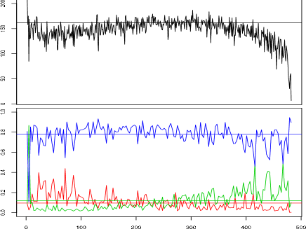
Figure 3: The same quantities as in Fig 2, except all the data was simulated from the effective model (3) by taking into account tail effects in the multivariate distribution via the one-factor stochastic volatility model BouchaudEtal_FatTailsRMT with tail index $\nu=3$.

Let us gain insight into the details of this correlation structure for the case of the data in Fig 1. By clustering analysis Mantegna_HierarchicalClust we find that $G_{23}$ separates further, $G_{23}=\{G_{23}^{+},G_{23}^{-}\}$, into two nearly-equally large groups of distinctly higher/lower mean average correlation with degeneracies $\{D_{23}^{+},D_{23}^{-}\}=\{29,32\}$ respectively. For this sample, we find that $G_{23}^{+}$ contains Electric Utilities, as well as Oil & Gas Drilling & Exploration stocks, while $G_{23}^{-}$ contains Oil & Gas Exploration, as well as some Financial stocks. From the average correlation between all four groups, we thus construct the following “minimal” coarse-grained effective model:

$$C_{eff}^{N\times N}=\left(\begin{array}[]{cccc}C_{23+}^{D_{23}^{+}\times D_{23}^{+}}&0.36&0.35&0.22\\ 0.36&C_{23-}^{D_{23}^{-}\times D_{23}^{-}}&0.33&0.20\\ 0.35&0.33&C_{\perp}^{D^{\perp}\times D^{\perp}}&0.20\\ 0.22&0.20&0.20&C_{1}^{D_{1}\times D_{1}}\end{array}\right)$$ (3)

which can be readily checked to be positive definite. The entries of each $D\times D$ diagonal block above are $C^{D\times D}=(1-\rho_{G})I_{D}+\rho_{G}^{D\times D},$ with $\{\rho_{23}^{+},\rho_{23}^{-},\rho_{\perp},\rho_{1}\}=\{0.59,0.48,0.32,0.13\}$ respectively being the average correlation of each of the four groups $G$ and $\rho_{G}^{D\times D}$ is a block whose entries are $\rho_{G}$. One can check that (3) also gives rise to $4$ distinct factors and $4$ distinct subbands.

Note that unlike the strongly correlated ones in $G_{23}$, the stocks in $G_{1}$ are typically not easily detectable with conventional hierarchical clustering approaches Mantegna_HierarchicalClust , although they are distinctly visible if one looks at the top factor (see Fig 1 inset). Indeed, being weakly correlated between each other as well as with the rest of the market, these stocks will not appear in localized real-space clusters but instead will group with other stocks in later stages of the hierarchy. At the same time, both the degeneracy $D_{1}$ and overal risk contribution of $G_{1}$ are comparable to those of the localized sectors, as also directly suggested by Fig 2 (b). To properly account for the separation of correlation scales in markets, one must also include the contribution of the weakly correlated stocks.

Simulating with tails:

A check of the validity of the effective model (3) is ultimately provided if one can reproduce the empirical spectrum and participations through simulation. To do so, one must properly take into account heavy tailed behavior of actual returns. It is known that such tails can be induced by heteroskedasticities of the underlying stock volatilities BouchaudPotters_book , although the details of the correlations of such volatility dynamics are not well understood. We thus use the simplest multivariate conditional Gaussian model with one-factor variance-gamma volatilities, which is known to produce a Student-t type of series BouchaudEtal_FatTailsRMT for the joint returns. We use an inverse-gamma tail index of $\nu\simeq 3$. The resulting spectrum BouchaudEtal_FatTailsRMT ; RMT_fatTailsOther agrees well with the empirical one. Moreover, comparing Figs 2 and 3, we see that the inverse participations are also in good agreement.

A Subtle Stationary Bias:

The discussion so far suggests that even for stationary data, RMT cleaning could produce biased risk estimates. Let us demonstrate this for the simplest case of multivariate Gaussian returns simulated with the effective model (3). Without loss of generality we normalize the returns to mean zero unit variance. Using the notation in PlerouEtal_PRE02 , the predicted risk of a portfolio $w=(w_{1},\ldots,w_{N})$ is $\Omega_{p}^{2}=w\cdot C_{clean}\cdot w^{T}$. The portfolios we look at are equal-weight average representatives of different subbands $K$, $w_{K}=\sum_{k\in K}e_{k}$, where $\{e_{k}\}$ are the eigenvectors of the effective model (3). Moreover, instead of a “budget constraint” PlerouEtal_PRE02 , we impose a “risk constraint” by normalizing $w_{K}$ to unit norm. We then compute at every forecasting period the relative difference between realized and predicted risk, $\delta r=(\Omega_{r}^{2}-\Omega_{p}^{2})/\Omega_{p}^{2}.$ For the subbands $\{K_{1},K^{\perp},K_{23}\}$ corresponding to the groups of stocks that enter in Fig 2 (b), we find respective biases $\delta r_{i}=\{26\pm 4\%,2\pm 4\%,-17\pm 2\%\}.$ Note that although $\delta r_{1}$ and $\delta r_{23}$ are significant, they are of opposite sign. Indeed, we have checked that all three contributions nearly cancel when one looks at the relative realized versus predicted risk of the entire noise band, $\delta r_{all}=2\pm 3\%$. Finally, we also observe significant biases $\delta r_{1}$ and $\delta r_{23}$ in the actual data. However, in this case, there are subtleties in disentangling the effects of multiple bands, tails, and non-stationarity. We postpone discussing these effects, as well as multi-residual generalizations of the RMT cleaning procedure to later work DimovShiber_unpublished .

Summary:

In conclusion, we have found strong evidence that instead of homogeneous, the stock market correlation residuals are composed of multiple subbands that do not fully mix. This structure is manifested through an asymmetry in the relative inverse participations of the eigenvectors within the noise band, which is inconsistent with purely symmetric cleaning that doesn’t distinguish between different parts of the noise spectrum. The multi-residual picture above natrually emerges from market models with multiple correlation scales, that we have identified and simulated. As a direct consequence, the scale separation within the noise band also produces inhomogeneities in the effective residual risk that in turn induce purely stationary biases of the original RMT cleaning.

- (1) M. L. Mehta, Random Matrices (Academic Press, Boston, 1991).
- (2) A. M. Sengupta and P. P. Mitra, Phys. Rev. E 60, 3389 (1999).
- (3) L. Laloux et al., Phys. Rev. Lett. 83, 1467 (1999).
- (4) V. Plerou et al., Phys. Rev. Lett. 83, 1471 (1999); V. Plerou et al., Phys. Rev. E 65, 066126 (2002).
- (5) A. Utsugi et al., Phys. Rev. E 70, 026110 (2004); V. Kulkarni and N. Deo, Europhys. J. B, 60, 101 (2007); R. Pan and S. Sinha, Phys. Rev. E 76, 046116 (2007); J. Shen and B. Zheng, Europhys. Lett. 86, 28005 (2009).
- (6) P. Gopikrishnan et al., arXiv:cond-mat/0011145 (2000).
- (7) M. Avellaneda and J-H Lee, Working Paper Series. Available at SSRN: http://ssrn.com/abstract=1153505.
- (8) V. Marčenko and L. Pastur, Math. USSR-Sbornik 1, 457 (1967).
- (9) G. Biroli et al., Europhys. Lett. 78 (No. 1), (2007); G. Biroli et al., Acta Phys. Pol. B 38 (13), 4009 (2007).
- (10) Z. Burda et al., Phys. Rev. E 71, 026111 (2005); Burda et al., Phys. Rev. E 74, 041129 (2006).
- (11) F. Lillo and R. N. Mantegna, Phys. Rev. E 72, 016219 (2005).
- (12) R. N. Mantegna, Europhys. J. B. 11 (No. 1), 193 (1999).
- (13) We have performed all the necessary tests BouchaudPotters_book to ensure that the marginal min midquote returns have no residual autocorrelations.
- (14) J.-P. Bouchaud and M. Potters, Theory of Financial Risk and Derivative Pricing (Cambridge Univ. Press, Cambridge, 2003).
- (15) After fitting for and one typically normalizes so as to preserve the conservation of the trace of correlations LalouxEtal00_RMT ; PlerouEtal_PRE02 .
- (16) M. Potters et al., Acta Phys. Pol. B 36 (9), 2767 (2005).
- (17) I. Dimov, D. Shiber, P. Kolm, L. Maclin in preparation.