From quasiperiodicity to high-dimensional chaos
without intermediate low-dimensional chaos

Abstract

We study and characterize a direct route to high-dimensional chaos (i.e. not implying an intermediate low-dimensional attractor) of a system composed out of three coupled Lorenz oscillators. A geometric analysis of this medium-dimensional dynamical system is carried out through a variety of numerical quantitative and qualitative techniques, that ultimately lead to the reconstruction of the route. The main finding is that the transition is organized by a heteroclinic explosion. The observed scenario resembles the classical route to chaos via homoclinic explosion of the Lorenz model.

Low-dimensional dissipative continuous systems, namely described by a d=3 phase space, may exhibit chaotic behavior, that may arise through a number of well characterized scenarios, including the route from quasiperiodicity to chaos and routes involving global bifurcations, like the route to chaos exhibited by the Lorenz system. Things become more complicated when the dimensionality of the phase space is increased. Interestingly, the limit in which one has an infinite-dimensional phase space, and the system exhibits the so-called spatio-temporal chaotic behavior, is well characterized through the ergodic theory of dynamical systems, through quantifiers like dimension, entropy, and Lyapunov exponents (a Lyapunov density in continuous systems). Less explored is the case in which one has a phase space that has an intermediate dimension between these two limits. In this case, one may have high-dimensional chaotic behavior, and an obvious possible route is a cascade in which the dimensionality of the high-dimensional attractor increases sequentially. Still, other possibilities may take place, like the scenario discussed in the present work, in which quasiperiodic attractors participate, though in a manner different to the classical quasiperiodic route to chaos. Instead, a high-dimensional chaotic attractor is created in a global bifurcation. Interestingly, the route exhibits a regime in which a three-dimensional quasiperiodic attractor is stable, in apparent contradiction to common wisdom interpretation of Ruelle-Takens-Newhouse Theorem.

I Introduction

Nonlinear dynamics was considerably boosted by the recognition of chaos as an ubiquitous phenomenon out of the linear realm. Chaos theory succeeded to identify the universal routes through which regular motion may become chaotic. In dissipative dynamical systems, chaos appears through a few well characterized routes (or scenarios) Eckmann (1981) like the following: (a) the period-doubling cascade Feigenbaum (1978); (b) the intermittency route Pomeau and Manneville (1980); (c) the route involving quasiperiodic tori Newhouse et al. (1978); Curry and Yorke (1977); (d) the crisis route Grebogi et al. (1983); (see also Bergé et al. (1986); Ott (1993) for a survey). Another possibility is that chaos sets in through a global connection to a fixed point, as is the case Sparrow (1982) of the Lorenz system, and of Shilnikov chaos Afraimovich et al. (1993); nat (1993).

More recently, some studies have been devoted to the study of high-dimensional chaos, that here we shall define as chaotic motion inside an attractor of typical dimension $d>3$ (as a typical one we may take the information dimension $D_{1}$). An obvious possibility to transit to high-dimensional chaos is to take as starting point a low-dimensional chaotic attractor. This possibility has been often considered in the context of desynchronization between coupled chaotic oscillators. A possible scenario, and probably the most studied one Harrison and Lai (1999); Kapitaniak et al. (2000) involves generating a hyperchaotic attractor—an attractor with two or more positive Lyapunov Exponents (LEs)—from a low-dimensional chaotic attractor. Another class of high-dimensional chaotic attractors exhibits two (at least very approximately) null Lyapunov exponents. As shown in Matías et al. (1997a); Sánchez et al. (2000); Yang (2000) one may encounter this situation in rings of asymmetrically (e.g. unidirectionally) coupled chaotic systems in which a symmetric Hopf bifurcation renders unstable the synchronized state Matías et al. (1997b); Matías and Güémez (1998).

Less obvious is the possibility of a direct transition to high-dimensional chaos without an intermediate low-dimensional chaotic attractor. Restricting to autonomous ordinary differential equations, the transition to high-dimensional chaos has been found to be associated to quasiperiodicity. Thus, the works by Feudel et al. Feudel et al. (1993) and Yang Yang (2000) report a transition from two- and/or three-frequency quasiperiodicity to high-dimensional chaos. A more geometrical view is in the work by Moon Moon (1997), that describes a route (to high-dimensional chaos) from a two-dimensional torus, through a global bifurcation that comprises a double homoclinic connection to a limit cycle (this structure amounts to adding one dimension to each building block of the homoclinic route to chaos in the Lorenz model). Recently Pazó and Matías (2005), we reported a route to chaos whose most novel aspect is that it implies the sudden creation (i.e. with no mediating low-dimensional chaos) of a high-dimensional chaotic attractor with $D_{1}>4$. In summary, in this route first a high-dimensional chaotic (nonattracting) set is created in a global bifurcation. Then, this set is rendered stable, becoming a high-dimensional chaotic attractor , in a boundary crisis.

The purpose of this paper is to explain in more detail our findings in Ref. Pazó and Matías (2005). In Sec. II the system is described and an overall picture of the route to high-dimensional chaos is presented. Then, Sec. III discusses at some detail the appearance and the robustness of the two- and three-frequency quasiperiodic attractors found in the system. Later, Sec. IV presents the numerical evidences that have been used to understand the complex route to chaotic behavior presented by the system. Section V presents a characterization of the route to high-dimensional chaos through a return map similar to that of the Lorenz system. The goal of Section VI is to present and discuss at some length the route to chaos exhibited by the system. Finally, Secs. VII and VIII present the final remarks on this work and the conclusions, respectively.

II System and overall picture

The system studied in the present work is a $9$-dimensional dynamical system considered here is formed by three Lorenz Lorenz (1963) oscillators coupled according to the partial replacement coupling method of Ref. Güémez and Matías (1995). The oscillators are unidirectionally coupled in a ring geometry such that,

$$\left.\begin{array}[]{rcl}\dot{x_{j}}&=&\sigma(y_{j}-x_{j})\\ \dot{y_{j}}&=&R\,\underline{x_{j}}-y_{j}-x_{j}\,z_{j}\\ \dot{z_{j}}&=&x_{j}\,y_{j}-b\,\,z_{j}\end{array}\right\}\quad j=1,\ldots,N=3\ ,$$ (4)

where $\underline{x_{j}}=x_{j-1}$ for $j\neq 1$, define the coupling, and $\underline{x_{1}}=x_{3}$ the ring geometry of the system. In our study two of the parameters are fixed as in Pazó et al. (2001); Pazó and Matías (2005)): $\sigma=20$, $b=3$, while $29<R<40$. The study of this system has been suggested by the results of the experimental study of rotating waves for three coupled Lorenz oscillators corresponding to these parameters Sánchez and Matías (1999); Sánchez et al. (2006).

A useful representation in the study and characterization of discrete rotating waves are the (discrete) Fourier spatial modes Heagy et al. (1994); Matías et al. (1997b). These modes are defined as,

$${\bf X}_{k}={1\over N}\sum_{j=1}^{N}{\bf x}_{j}\exp\left[{{2\pi i(j-1)k}\over N}\right]\ ,$$ (5)

where $N=3$ (as already indicated) and $i$ is the imaginary unit. In terms of these modes (${\bf X}_{0}\in\mathbb{R}^{3},{\bf X}_{1}\in\mathbb{C}^{3}$), the evolution equations are,

$$\left.\begin{array}[]{rcl}\dot{X_{0}}&=&\sigma(Y_{0}-X_{0})\\ \dot{Y_{0}}&=&R\,X_{0}-Y_{0}-X_{0}\,Z_{0}-X_{1}\,Z_{1}^{*}-X_{1}^{*}\,Z_{1}\\ \dot{Z_{0}}&=&X_{0}\,Y_{0}-b\,\,Z_{0}+X_{1}\,Y_{1}^{*}+X_{1}^{*}\,Y_{1}\\ \dot{X_{1}}&=&\sigma(Y_{1}-X_{1})\\ \dot{Y_{1}}&=&{\tilde{R}}\,X_{1}-Y_{1}-X_{0}\,Z_{1}-X_{1}\,Z_{0}-X_{1}^{*}\,Z_{1}^{*}\\ \dot{Z_{1}}&=&X_{0}\,Y_{1}+X_{1}\,Y_{0}-b\,\,Z_{1}+X_{1}^{*}\,Y_{1}^{*}\end{array}\right\}\$$ (12)

with ${\tilde{R}}=R\exp(2\pi i/3)$, and where $X_{1}^{*}$ denotes the complex conjugate of $X_{1}$.

The qualitative description of the behaviors exhibited by the system in this range of parameters is as follows. The three Lorenz oscillators exhibit chaotic synchronization for $R<R_{sc}\approx 32.82$. At $R_{sc}$ the system exhibits a Hopf bifurcation directly from a chaotic state, yielding a behavior, that was first found in rings of unidirectionally coupled Chua’s oscillators and called a Chaotic Rotating Wave (CRW) Matías et al. (1997a). The Hopf bifurcation exhibited by the system is called symmetric Golubitsky and Stewart (1985); Collins and Stewart (1994), as it originates from the cyclic ($\mathbf{Z}_{3}$) symmetry of the ring. Close to the bifurcation the CRW is the combination of the chaotic dynamics in a Lorenz attractor and a superimposed oscillation created by the Hopf bifurcation, that occurs in the subspace transverse to the synchronization manifold ($k=1$ mode). The oscillation created in the symmetric Hopf bifurcation is characterized by a phase difference of $2\pi/3$ ($2\pi/N$ in the general $N$-oscillator case) between neighbor oscillators, and this behavior is the discrete analog of a traveling rotating wave Aronson et al. (1991). This picture is valid close to onset, $R\gtrsim R_{sc}$, and when increasing $R$ one observes that this behavior changes. For $R>35.26$ the behavior of the system becomes periodic, with a waveform characteristic of the $k=1$ Fourier mode. Actually, two mirror limit-cycle attractors, called Periodic Rotating Wave (PRW) in Ref. Matías et al. (1997b); Sánchez and Matías (1998), are found in the range $R\in[35.26,39.25]$ (approximately). At $R=R_{pitch}\approx 39.25$ both solutions merge giving rise, through a pitchfork bifurcation, to a centered stable symmetric periodic behavior.

We shall not describe here the transition from synchronous chaos to CRW; instead, we shall focus on the transitions from PRW to CRW, i.e. we go ‘from order to chaos’ decreasing $R$. The reader should notice that by CRW we refer to a high-dimensional chaotic attractor characterized by a oscillation with a $2\pi/3$ phase shift between neighboring oscillators superimposed to an underlying chaotic behavior. The temporal series for the different behaviors studied in this work are shown in Fig. 1. Note that the third frequency, that appears as the $\mathbb{T}^{3}$ is born, manifests as a very slow modulation on the size of the former $\mathbb{T}^{2}$ (the time scale has been broadened in Fig. 1(c) in order to allow the observation of this slow scale).

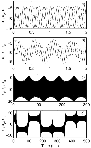
Figure 1: Time series of the system Eq. (4): (a) $R=35.5$, Periodic Rotating Wave; (b) $R=35.2$, $\mathbb{T}^{2}$; (b) $R=35.095$, $\mathbb{T}^{3}$; (d) $R=35.093$, Chaotic Rotating Wave. Note the different time scale for each panel.

A view of the parameter region that will be considered in this work can be found in Fig. 2, in which the Lyapunov spectrum corresponding to the four largest Lyapunov exponents is presented. From right to left, the two symmetry-related limit-cycle attractors exhibit a (supercritical) Hopf bifurcation when $R$ is decreased, namely at $R=R_{h1}\approx 35.26$, yielding two symmetry-related two-frequency quasiperiodic attractors (with two null LEs). Lowering $R$ further the system exhibits another (supercritical) Hopf bifurcation, at $R=R_{h2}\approx 35.0955$, that yields two mirror three-frequency quasiperiodic attractors (three vanishing LEs). Lowering $R$ furthermore the system exhibits a boundary crisis, at $R=R_{bc}\approx 35.09384$, in which the chaotic attractor is born (or destroyed seen from the opposite side). The chaotic attractor is characterized by two vanishing (at least, very approximately) Lyapunov exponents, and a single positive LE that is larger than the absolute value of the fourth LE. This implies, according to the Kaplan-Yorke conjecture, that the information dimension $D_{1}>4$. As we shall see below (see Sec. IV.4) this dimension is genuine.

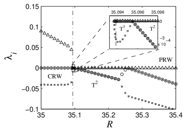
Figure 2: The four largest Lyapunov exponents ($\lambda_{i=1,...,4}$) as a function of the parameter $R$. Four regions can be distinguished according to their different Lyapunov spectra. Note that for the high-dimensional chaos we obtain $\lambda_{2}=\lambda_{3}=0$ and $\lambda_{1}\gtrsim|\lambda_{4}|$ which implies, according to the Kaplan-Yorke conjecture, an information dimension $D_{1}\gtrsim 4$. The dash-dotted line indicates the value of $R$ where the chaotic attractor is born.

The presence of 2-D and 3-D quasiperiodic attractors may lead to think that chaos appears through a quasiperiodicity transition to chaos (see Sec. III). However, it will be shown below that the chaotic attractor is created at a boundary crisis, and coexists with the two $\mathbb{T}^{3}$ attractors until the latter are destroyed as each of them collides with a twin unstable $\mathbb{T}^{3}$, at $R=R_{sn}=35.09367$. We shall show (from Sec. IV) that, indeed, the system exhibits a global bifurcation —analogous to what happens for the Lorenz system Sparrow (1982)— that implies, in first approximation, the sudden creation of an infinite number of unstable 3-D tori.

A schematic diagram of the whole set of bifurcations linking the PRW and synchronous chaos is shown in Fig. 3. As mentioned above, in the interval of $R$ where the CRW is found, the shape of the attractor changes. Anyway, in this paper we are not interested in the transitions between different types of chaotic rotating wave (see Sánchez et al. (2006) for such a study).

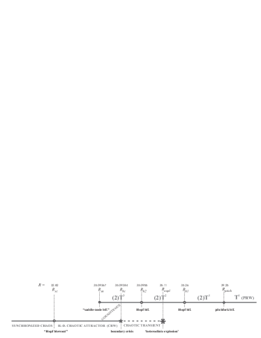
Figure 3: Diagram representing schematically the transitions from synchronous chaos (left) to a PRW (right).

III Transition to Quasiperiodic behavior

As described above, the (symmetric) periodic rotating wave, that is the starting point of our analysis, is replaced after a sequence of bifurcations by two mirror three-frequency quasiperiodic attractors, $\mathbb{T}^{3}$. The involved transitions are a pitchfork bifurcation, in which two (asymmetric) periodic rotating waves are born, and then two consecutive Hopf bifurcations. A small note is in place about the stability of this type of unusual attractors as it has been stated that $\mathbb{T}^{3}$ attractors are intrinsically fragile according to Newhouse-Ruelle-Takens (NRT) Theorem Newhouse et al. (1978).

First of all, one can present numerical evidence to show that, indeed, three-frequency quasiperiodic attractors are observed robustly in a finite parameter range. In particular the inset of Fig. 2 shows results corresponding to the calculation of the Lyapunov spectrum in the $\mathbb{T}^{3}$ parameter range. As there are long chaotic transients in this region, the calculations were performed using long transients (of the order of $10^{6}$ t.u.), while another $10^{6}$ t.u. were used to calculate the spectrum.

On the other hand, and as already reported in Ref. Pazó et al. (2001), it can be numerically checked that the system exhibits three-frequency quasiperiodic behavior by looking at the Poincaré cross section of a $\mathbb{T}^{3}$ torus in phase space. Namely, in Fig. 2 of Ref. Pazó et al. (2001) the Poincaré sections of a $\mathbb{T}^{2}$ and of a $\mathbb{T}^{3}$ torus, respectively, are presented. While the former is a circle, the latter is clearly a two-dimensional, $\mathbb{T}^{2}$, torus. In the literature Ref. Yang (2000) reports the existence of three-frequency quasiperiodicity in a ring of coupled Lorenz oscillators (in a different parameter regime), while a case of a third very low frequency associated to a $\mathbb{T}^{3}$ torus has been observed in Refs. Wang and Nicolis (1987); Lopez and Marques (2000); Marques et al. (2001).

In trying to justify the robust existence of $\mathbb{T}^{3}$ dynamics in the light of the NRT Theorem, a first observation is that in our simulations we have not detected resonances in the $\mathbb{T}^{2}$ regime. This may occur due to the fact that along $R$, the winding number does not crosses hard resonances, the smallest denominator is $q=11$ (corresponding to a winding number of $4/11$), so the resonance horns may be quite small. But also it is important to notice that the absence of resonances in rotating waves is a characteristic feature of systems with rotational, $SO(2)$, symmetry Rand (1982). For instance in a homogeneous excitable medium, the compound rotation of a spiral wave lacks of frequency lockings due to this symmetry Barkley (1995). Therefore the stability of the $\mathbb{T}^{3}$ attractors would be subsequent to the robustness of the quasiperiodic dynamics on the two-tori. In a sense our three-frequency quasiperiodic attractors would be as robust as two-frequency quasiperiodic attractors. It is clear that in our system this rotational symmetry is only approximate, but one may consider the discreteness effect as a small perturbation. Also the third frequency is very small what precludes strong resonances with small denominators: thus, for $R=35.095$ [Fig. 1(c)] we have $f_{1}=5.3\ldots$, $f_{2}=1.87\ldots$, and $f_{3}=0.016\ldots$. These arguments support the existence of a range of three-frequency quasiperiodic behavior.

IV Numerical evidences of the route to chaos exhibited by the system

In this section we are going to analyze the route through which a chaotic attractor is born in this system. First of all, we shall reduce the dimensionality of the problem by eliminating the fast frequency, namely the one involved in the phase shift by $2\pi/3$ in neighbor oscillators, as it leads to a conserved quantity (this time lag) and consequently a vanishing (or almost vanishing) Lyapunov exponent. In the mode representation of Eq. (12) this amounts to perform a cut through the Poincaré section $Im(X_{1})=0,Im({\dot{X}}_{1})>0$. So, in visualizing objects cycles will become fixed points, $\mathbb{T}^{2}$-tori cycles and $\mathbb{T}^{3}$-tori will become $\mathbb{T}^{2}$-tori, although we shall refer to these objects corresponding to the complete phase space, and not to the result of the dimensionality reduction achieved via sectioning.

IV.1 Coexistence between 3D-torus and CRW

The first important remark about our system of three coupled Lorenz oscillators is that the two $\mathbb{T}^{3}$ attractors are not directly involved in the birth of the high-dimensional chaotic attractor. Continuation of the $\mathbb{T}^{3}$ attractors shows that they exist above $R_{sn}=35.09367$. This implies that the system exhibits multistability between the high-dimensional chaotic and the $\mathbb{T}^{3}$ attractors in the range $R_{sn}<R<R_{bc}$, with the latter attractors having a small basin of attraction. This remark is important, because it implies that the high-dimensional chaotic attractor is not created through some route involving the $\mathbb{T}^{3}$ attractors.

Figure 4: Blowout of the four largest Lyapunov exponents for the $\mathbb{T}^{3}$ attractors in the region in which they coexist with the chaotic attractor. The fourth Lyapunov exponent approaches zero in a square-root fashion, as expected for a saddle-node bifurcation.

A detailed view of the behavior of the four largest Lyapunov exponents for the $\mathbb{T}^{3}$ attractors is represented in Fig. 4. It can be seen that close to $R_{sn}$ the fourth Lyapunov exponent exhibits a square-root profile as expected for a saddle-node bifurcation. This suggests that each $\mathbb{T}^{3}$ attractor is approaching an unstable $\mathbb{T}^{3}$. Also one can appreciate quite clear lockings where the third and fourth Lyapunov exponents become equal.

As $R$ approaches $R_{sn}$ the existence of a smooth invariant 3D-torus cannot be guaranteed, because the strength of the normal contraction can be of the same order than the rate of attraction of the 2D-torus arising in each locking Chow and Hale (1982). Thus, in Fig. 5 a possible scenario for the interaction of the tori, that would explain the lockings observed in Fig. 4 is presented. Because of the extremely small transversal stability of the $\mathbb{T}^{3}$ (represented by the fourth exponent), for $R\gtrsim R_{sn}$, we conjecture that the transversal direction ‘slaves’ the tangential one (represented by the third exponent). Then, we observe two identical non-vanishing exponents that may indicate the existence of a stable focus-type $\mathbb{T}^{2}$ on the surface of the $\mathbb{T}^{3}$. The $\mathbb{T}^{3}$ continues to exist but is non-differentiable at the stable $\mathbb{T}^{2}$ located on its (hyper)surface.

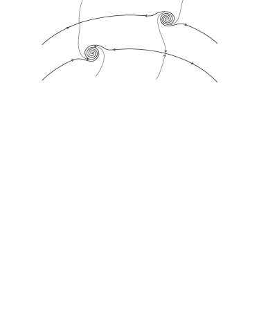
Figure 5: Schematic of a ‘slave locking’. A portion of a section of the tori (stable and unstable) are shown with bold lines. Tori are not differentiable at the foci.

The participation of the unstable 3D-torus in the final annihilation of the stable one is not trivial (the existence of the unstable $\mathbb{T}^{3}$ is supported by another numerical evidence, discussed in Sec. IV.5), but we want to recall that saddle-node bifurcations of $\mathbb{T}^{2}$ tori have been reported Ashwin (1998) (called bubbles in this reference), and due to the special character of the $\mathbb{T}^{3}$ tori that we have here (with one oscillation that, in some sense, is orthogonal to the others and also almost conserved, cf. Sec. III), and given the numerical evidence reported here, we think that we have found a saddle-node bifurcation of $\mathbb{T}^{3}$ tori.

IV.2 Route to chaos in the Lorenz model through homoclinic explosion and boundary crisis

As the route studied in this work presents some similarities with the classical route to chaos for an isolated Lorenz system, we are going to draw some useful analogies with that system, although it is warned that the analogy is not complete (otherwise, we would not have a new route to chaos). As it can be found in textbooks Ott (1993), the Lorenz system exhibits several routes to chaos. The classical one is the route to chaos through a double homoclinic connection of the saddle point at the origin. Fixing $\sigma$ and $b$, the double homoclinic orbit occurs at a particular value $R=R_{HOM}$. It has the shape of the butterfly (taking into account how the unstable directions reenter the saddle point at the origin, being this dictated by the reflection symmetry of the system), and this gives birth Afraimovich et al. (1993) to a chaotic set for $R>R_{HOM}$ (a homoclinic explosion Yorke and Yorke (1979); Sparrow (1982)). The closure of this set is formed by the infinite number of unstable periodic orbits (UPOs) that can be classified according to their symbolic sequences of turns around the right ($\mathbf{R}$) and the left ($\mathbf{L}$) fixed points ($C_{+}$ and $C_{-}$) Sparrow (1982). The appearance of these UPOs reflects the dramatic change undergone by the stable manifold of the fixed point that allows initial conditions at one side of the phase space jump to the other side (before falling to one of the two symmetry related stable fixed points $C_{+}$ and $C_{-}$), being these jumps impossible for $R<R_{HOM}$. For a larger value of $R$, $R=R_{BC}$, the chaotic set becomes stable in a boundary crisis, that occurs precisely when the two shortest symmetry-related length-$1$ unstable periodic orbits ($\mathbf{R}$ and $\mathbf{L}$) located at each lobe, and that at $R=R_{HOM}$ coincide with the two homoclinic orbits, shrink, such that the chaotic set has a tangency with these two orbits Sparrow (1982). At this value of $R$ there exists a double heteroclinic connection between the equilibrium at the origin and the mentioned length-$1$ UPOs. For $R_{BC}<R<R_{H}$ these two orbits (and their respective tubular stable manifolds) form the basin boundaries between the chaotic attractor and the two stable asymmetric fixed points $(C_{\pm})$, and, consequently, the system exhibits multistability. These two fixed points loose their stability in a a subcritical Hopf bifurcation, that occurs when the two mentioned length-$1$ orbits shrink to a point coinciding with $(C_{+},C_{-})$.

IV.3 Heteroclinic explosion

In our system one can find a value of $R=R_{expl}\approx 35.11$ that defines a clearcut transition in the way in which transients approach the attractors (that for $R\sim R_{expl}$ are two $\mathbb{T}^{2}$-tori). For $R>R_{expl}$ the basin of attraction of each $\mathbb{T}^{2}$ is quite simple. But below $R_{expl}$ trajectories may tend asymptotically to one of the $\mathbb{T}^{2}$ after visiting the neighborhood of the other torus.

Following the analogy with the Lorenz system, we conjecture that precisely at $R=R_{expl}$ a global bifurcation occurs, and past this value ($R<R_{expl}$) an infinite number of unstable objects are created. To check this we stabilized the symmetric PRW (an unstable fixed point in the Poincaré map) by a Newton-Raphson method and observed the fate of the trajectories starting from (approximately) that solution. In Fig. 6 the evolution of the trajectories for two values of $R$ above and below $R_{expl}$ is shown. After approaching one the asymmetric PRWs (its location is marked with a bold dotted line) the trajectory jumps or not to the other side. The result obtained for $R_{expl}$ is the same if one takes as starting point one of the asymmetric PRWs.

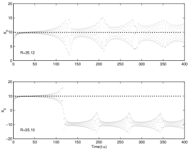
Figure 6: Numerical experiment showing the time series of the coordinate $X_{0}$ at the Poincare section for trajectories starting in an initial condition in the symmetric unstable PRW: (a) for $R=35.12$, a condition before the explosion (b) for $R=35.10$ just past the explosion. The $X_{0}$ coordinate of one of the two asymmetric PRWs is denoted with a bold dotted line.

IV.4 Four-dimensional branched manifold

The third important numerical remark refers to the Lyapunov spectrum (Table I) of the different attractors in the multistability region (of course, and due to symmetry, the Lyapunov spectra of the two $\mathbb{T}^{3}$ attractors are identical). As one can see, fifth to ninth LEs are quite similar, indicating that both attractor types are approximately embedded in the same four-dimensional space, a subset of the total phase space.

$\lambda_{i}$	CA	$\mathbb{T}^{3}$
$\quad\lambda_{5}\quad$	$\quad-5.254(7)\quad$	$\quad-5.202(7)\quad$
$\lambda_{6}$	$\quad-5.254(8)\quad$	$\quad-5.202(7)\quad$
$\lambda_{7}$	$\quad-18.612(4)\quad$	$\quad-18.651(9)\quad$
$\lambda_{8}$	$\quad-18.612(4)\quad$	$\quad-18.651(9)\quad$
$\lambda_{9}$	$\quad-24.273(4)\quad$	$\quad-24.290(4)\quad$

TABLE I: The five smallest Lyapunov exponents for the two attractors (CA: chaotic, and $\mathbb{T}^{3}$: three-frequency quasiperiodic) coexisting at $R=35.0938$.

Thus, we postulate that the dynamics can be simplified to the study of a four-dimensional branched manifold. A theoretical justification of this statement is impossible, but one can argue along the lines of (a higher-dimensional generalization of) the Birman-Williams Theorem Gilmore (1998); Birman and Williams (1983) (this theorem has proven to be very useful, even if it requires the strange attractors to be (uniformly) hyperbolic what is usually not fulfilled; notice, however, some recent rigorous advances Araujo et al. (2009) on the theory of singular hyperbolic attractors, that encompass the Lorenz equations Lorenz (1963).

In our case we can argue that the high-dimensional chaotic attractor has, according to Kaplan-Yorke conjecture Kaplan and Yorke (1979a), a value of the information dimension $D_{1}\gtrsim 4$ (cf. Fig. 2). We have also measured the correlation dimension $D_{2}$ (through Grassberger-Procaccia algorithm) obtaining also a value close to $4$, namely $D_{2}=3.96\pm 0.05$), (recall that $D_{1}\geq D_{2}$).

A more correct picture of the attractor amounts to consider that this $4$-dimensional manifold is actually composed of many thin leaves. Of course this reduced $4$-dimensional picture can be only considered to be a more or less faithful representation of the system. In the epochs in which a trajectory jumps to the other side (subspace), which means reinjections through an extra dimension, it is when the existence of branching is needed in order to the trajectory not to intersect itself. In our case the ‘tear point’ is the symmetric PRW. This is in complete analogy with what happens with the Lorenz system, where the attractor can be understood as a template composed of a branched two-dimensional manifold with a tear point at the origin (cf. Fig. 20(b) in Gilmore (1998)). Rotations around one of the lobes are roughly planar, but reinjections between the two (planar) lobes, that form themselves an angle, involve the third dimension.

An important remark concerning this $4$-dimensional picture is that, in this space, a $\mathbb{T}^{3}$-torus divides a $4$-dimensional manifold in two regions (just the same as a cycle divides a surface). Then in the regime with coexistence, between chaos and three-frequency quasiperiodicity, it is the pair of (conjectured) unstable 3D-tori what defines the basin boundary of the chaotic attractor. In the Lorenz system the length-$1$ unstable periodic orbits divide the $2D$-manifold in three regions; and also they acts as the basin boundaries, when the chaotic and the fixed point attractors coexist. In the transient chaos region, trajectories spiral in one lobe away from the fixed point (say $C_{+}$) because of the repulsive effect of the UPO surrounding that fixed point. After some turns the trajectory jumps to the other lobe by using the third dimension (i.e. by virtue of the branching). If the trajectory approaches close enough to $C_{-}$ surpassing the ‘barrier’ constituted by the length-$1$ UPO, it is captured by this fixed point and no more jumps occur (i.e. the chaotic transient finishes). Analogously, the unstable $\mathbb{T}^{3}$-torus acts as a dividing hypersurface for trajectories in the $4$-dimensional branched manifold, as discussed above.

IV.5 Boundary crisis and power law of chaotic transients

The fourth remark regards numerical studies for $R\gtrsim R_{bc}$. We have measured the average time of the chaotic transients ($\left<\tau\right>$) when approaching $R=R_{bc}$. We observe that these transients diverge satisfying a power law ($\left<\tau\right>\propto(R-R_{bc})^{\gamma}$), with $\gamma=-1.53\pm 0.06$, for an asymptotic value $R=R_{bc}=35.093838$, as expected for a boundary crisis Grebogi et al. (1987), see Fig. 7.

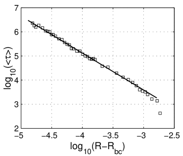
Figure 7: Log-log representation of the average chaotic transient as a function of the distance to the critical point $R_{bc}$. Each point is an average over 100 realizations. Data fit to a straight line of slope $\gamma=-1.53\pm 0.06$.

Inspired in the boundary crisis occurring in the Lorenz system Kaplan and Yorke (1979b); Grebogi et al. (1987); Sparrow (1982), we took one initial condition in one of the asymmetric (already unstable) Periodic Rotating Waves for different values of $R$. When $R$ is above $R_{bc}$ (but below $R_{expl}$), the system goes away of the limit cycle (due to numerical roundoff errors), and jumps to the $\mathbb{T}^{2}$ (or $\mathbb{T}^{3}$) attractor located at the other side of phase space. Contrary to what happens to typical initial conditions for those $R$ values, the chaotic transient is not observed, as may be seen in Fig. 8 (the PRW is a fixed point in the figure, as it has been stroboscopically cut through the Poincaré hyperplane $Im(X_{1})=0$). For $R$ just above $R_{bc}$ (cf. Fig. 8) the trajectory seems to approach a $\mathbb{T}^{3}$ before ‘falling’ to the $\mathbb{T}^{3}$ attractor. Thus, we conjecture that is the unstable $\mathbb{T}^{3}$ which constitutes the basin boundary of the chaotic attractor and the object involved in a global connection that marks the birth (or the death, depending on the viewpoint) of the chaotic attractor. Notice also, that the stable and the unstable $\mathbb{T}^{3}$-tori have quite similar sizes. Ultimately, at $R_{sn}$, the multistability region has an end when the two $\mathbb{T}^{3}$-tori annihilate in a saddle-node bifurcation (actually there are two mirror bifurcations, as previously discussed in Sec. IV.1).

Figure 8: Numerical experiment showing a trajectory (only points at the Poincaré section are shown) starting in an initial condition at one of the asymmetric unstable PRWs for $R=35.09389\gtrsim R_{bc}$. The unstable 3D-torus, larger, is seen initially, but finally (part (b)) the system decays to the smaller stable 3D-torus. Note that the minimum width along time is larger for the stable 3D-torus as expected for a torus located inside another (see the discussion about the branched manifold).

V Description in terms of a return map

Lorenz Lorenz (1963) described a nice technique for reducing the complexity of the solutions of the Lorenz equations. By recording the successive peaks of the variable $z(t)$, he reduced the dynamics of the Lorenz system to a one dimensional map. Denoting the $n$th maximum of $z(t)$ by $M_{n}$, he plotted successive pairs ($M_{n},M_{n+1}$), finding that points lay (very approximately) along a $\Lambda$-shaped curve. In this way, the dynamics is reduced to the “Lorenz map”: $M_{n+1}=\Lambda(M_{n})$.

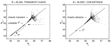
Figure 9: Return map of the maxima of the variable $Z_{0}$ satisfying to be larger than their adjacent maxima (see text). The left panel shows a regime of transient chaos; after a transient the trajectory decays to the stable $\mathbb{T}^{3}$ (following the dotted arrows). As $R$ is decreased the stable and the unstable $\mathbb{T}^{3}$ get closer. Beyond some point ($R<R_{bc}$) orbits inside the chaotic set do not escape, which means that the chaotic set has become an attractor. The right panel shows the attractors occurring for $R$ into the coexistence interval.

In our case we may try to reduce the dynamics by means of a return map. The fast dynamics concerning the $k=1$ mode is approximately filtered when considering the $k=0$ mode. Then, the $\mathbb{T}^{3}$ attractor is seen in the $k=0$ framework as a $\mathbb{T}^{2}$ plus some small residual oscillating component. A return map of the variable $Z_{0}$ would reduce the dimension of the attractors by one, and giving as a result an (approximately) one dimensional curve for the $\mathbb{T}^{3}$ attractor. We must take an additional return map to reduce the $\mathbb{T}^{3}$ to a fixed point, and the chaotic set of dimension (about) four to a line. Considering the set of maxima of $Z_{0}(t)$, $\{M_{n}\}$, we took the subset of maxima whose neighboring maxima were smaller: $\{N_{j}\}=\{M_{n}>M_{n\pm 1}\}$, what effectively amounts to consider the maxima of the low frequency oscillations. The results for two values of the parameter $R$ at both sides of the crisis ($R=R_{bc}$) are shown in Fig. 9. The chaotic attractor exhibits a rough $\Lambda$-shaped structure as occurs with the Lorenz map. Probably, the existence of the residual fast component makes the attractor to deviate significantly from one-dimensionality. In the light of the paper by Yorke and Yorke Yorke and Yorke (1979), who studied the transition to sustained chaotic behavior in the Lorenz model with the Lorenz map, it is found that our results are consistent with a boundary crisis mediated by an unstable three-torus.

VI Route to chaos: theoretical analysis

Condensing all the information obtained from numerical experiments in the previous sections, we suggest the route to high-dimensional chaos represented in Fig. 10 (where it is to be understood that the customary cross section through the fast rotating wave is applied). The high dimension of our attractor makes somewhat convoluted a geometric visualization. As we explained above, we postulate a chaotic attractor whose structure may be simplified in terms of a 4-dimensional branched manifold, and therefore the Poincaré section reduces the attractor to a 3-dimensional branched manifold. Figure 10 represents a projection onto $\mathbb{R}^{3}$, hence some (apparently) forbidden intersections between trajectories appear because of the branching. As occurs with the Lorenz attractor when it is projected on $\mathbb{R}^{2}$ (say $x-z$), the intersections between trajectories coming from different lobes, and also of them with the $z$ axis (that belongs to the stable manifold of the origin) are unavoidable. Recall that it is the moment of the jump when the extra dimension is needed, and this is provided by the definition of a branched manifold.

Figure 10: Three-dimensional representation of the proposed heteroclinic route to create the high-dimensional chaotic attractor. Black and gray points correspond to stable and unstable fixed points (cycles in the global phase space), respectively. This representation is obtained through a Poincaré cross section of the real attractors of the system, that eliminates the (fast) oscillation along the ring.

Summing up our previous numerical findings, we have for descending values of $R$: the centered PRW (a) becomes unstable through a pitchfork bifurcation (a$\rightarrow$b) and two symmetry-related PRWs appear (b). At a supercritical Hopf bifurcation (b$\rightarrow$c) the $\mathbb{T}^{2}$ appears. When $R$ is slightly decreased the 2D-torus becomes focus-type (d); the leading Lyapunov exponent becomes degenerate as may be seen in Fig. 2. Hence the unstable manifold of the asymmetric PRW forms a ‘whirlpool’ Shilnikov et al. (1995) when approaching the $\mathbb{T}^{2}$. At $R_{het}$ a double heteroclinic connection between the asymmetric PRWs and the symmetric one occurs (e) (only the upper half of the connection is shown for clarity). At this point the chaotic set is created, that includes a dense set of unstable 3D-tori. In (f) the two simplest 3D-tori are represented with dotted lines, because of the heteroclinic birth one of the frequencies of these tori is very small. Note that the plot shows that the unstable manifold of one of the asymmetric PRWs intersects the stable manifold of the symmetric PRW which in principle violates the theorem of existence and uniqueness. This occurs, as we said above, because we are projecting the Poincaré section onto $\mathbb{R}^{3}$ (one could imagine this as our particular Flatland. Twin secondary Hopf bifurcations (f$\rightarrow$g) render unstable the 2D-tori and give rise to two stable $\mathbb{T}^{3}$ (g). When $R$ is further decreased the asymmetric PRWs are not connected by their unstable manifolds to the $\mathbb{T}^{3}$ (h), and the chaotic set becomes attracting.

A two-dimensional cut of the schematic shown in Fig. 10 is depicted in Fig. 11. Only some of the subplots of both figures are one-to-one related. Specifically, Fig. 11(h) corresponds to $R=R_{bc}$, whereas Fig. 11(i) corresponds to $R=R_{sn}$.

It is to be stressed that the existence of $\mathbb{T}^{3}$ attractors is not a fundamental part of the transition to high-dimensional chaos. Just focus type $\mathbb{T}^{2}$ are needed such that the unstable manifolds of the asymmetric PRWs form whirlpools Shilnikov et al. (1995). In this way, regarding the chaotic attractor, no fundamental change occurred if the unstable $\mathbb{T}^{3}$ shrank to collide with the stable $\mathbb{T}^{2}$ in a subcritical Neimark-Sacker bifurcation. This picture would be more similar to the transition in the Lorenz system where $C_{\pm}$ become unstable through a subcritical Hopf bifurcation.

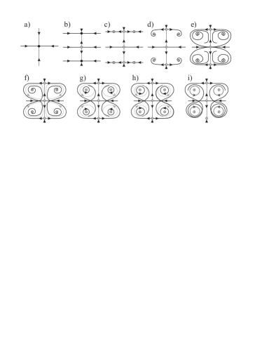
Figure 11: Two-dimensional representation of the proposed heteroclinic route to create the high-dimensional chaotic attractor. It represents a vertical cut of Fig. 10. $\odot$ (resp. $\circledcirc$) symbols represent stable (resp. unstable) periodic orbits (2D-tori in the full phase space).

VII Further remarks

In this section we want to address some subtle aspects concerning the transition to chaos shown in this paper.

The first point that must be noted is that Fig. 10 is representing a map (instead of a continuous dynamical system) because a Poincaré section of the fast dynamics involving the spatial mode is assumed. However the fast spatial frequency is somehow ‘orthogonal’ along the transition and therefore phase space may be understood as a direct product of this frequency with the transition shown in Fig. 10 that can be assumed not to differ too much from a continuous system. The fast spatial rotating wave is approximately conserved along the transition (cf. Sec. III), and the weak interaction of this frequency stems from the rotational symmetry of the system and manifests through an additional vanishing Lyapunov exponent in the high-dimensional chaotic region.

Let us consider further which is the meaning of the Lyapunov spectrum of the chaotic region. According to the route described by Figs. 10 and 11 an infinite number of unstable $\mathbb{T}^{3}$ are created at the heteroclinic explosion (recall that only the two simplest ones are shown). Hence, we could expect to have a chaotic attractor with three vanishing Lyapunov exponents. Why only two are observed? (cf. region CRW in Fig. 2).

One could be tempted to think that that due to the non-hyperbolicity of quasiperiodic behavior, a finite ratio of the 3D-tori set corresponds to locked tori (probably with large denominators), contributing to shift the vanishing Lyapunov exponents from zero. However we believe that the absence of a third vanishing Lyapunov exponent is due to the following. It must be noted that the heteroclinic connection between the symmetric and the asymmetric PRWs is structurally unstable. Nonetheless, we have numerically observed (see Fig. 6) that the connection (approximately) persists. Also, the axial symmetry of Fig. 10 has not a theoretical justification. In our view the situation is similar to the study of codimension-$m$ ($m>1$) bifurcations, where an increase of the highest order $n<n_{max}$, of the terms constituting the normal form (or $n$-jet) or adding a non symmetric term, makes substructures in the bifurcation sets emanating from the codimension-$m$ point to appear. For example, the effect of including non-axisymmetric terms to the normal form of the saddle-node Hopf (codimension-two) bifurcation has been studied by Kirk Kirk (1991).

Hence we expect that, a perturbation on the mechanism shown in Fig. 10 will break the symmetry that allows such a “simple” picture. Inspired on previous works Kirk (1991); Gaspard (1993) dealing with the effect of non-symmetric terms on codimension-two bifurcations, we postulate that homoclinic connections would replace heteroclinic connections. A double (‘figure-eight’) homoclinic of the symmetric PRW as well as homoclinic connections of the asymmetric PRWs would occur. Symmetric and asymmetric PRWs are both saddle-foci so we computed their saddle indices finding that a (Shilnikov) chaotic set should arise.

The existence of homoclinic chaos (with the only novel feature of having a superimposed fast spatial wave) could be considered as uninteresting and well known (see e.g. Arneódo et al. (1981)). But it is to be emphasized that as the exact mechanism is very related to what shown in Fig. 10, the first negative Lyapunov exponent is very close to zero which makes the information dimension to be larger than four (or larger than three if the spatial oscillation is considered extra and/or trivial).

The next question is how the two simplest unstable 3D-tori appear if the route is not exactly as appears in Fig. 10. A possibility is that they appear though a saddle-node bifurcation between two unstable 2-tori (see footnote 6 for its plausible origin), but we have no way to find out this.

It is well known, Guckenheimer and Holmes (1983); Kuznetsov (1998); Gaspard (1993) that global bifurcations and complex behavior have in many cases a local origin, namely a high codimension point. at which the loci of several bifurcations meet in parameter space. In particular, a Gavrilov-Guckenheimer (or saddle node-Hopf point) yields, among other, quasiperiodic dynamics. The reflection symmetry of the model studied in this work would imply the possibility of a pitchfork-Hopf interaction in this case. Although the unfolding for this codimension-$2$ point has not been fully characterized, it could be a clear candidate as an organizing center of part of the complex behavior discussed in this work. However, the location of such hypothetical critical point is rendered more difficult by the fact that, due to the presence of a spatial frequency in all the relevant parameter region, the hypothetical pitchfork-Hopf point would occur in a Poincaré cross section of the system, making all the analysis much more involved. In particular, we have tried this avenue of research without success, and, thus, we have not been able to find a coalescence of the loci of the pitchfork and Hopf bifurcations.

VIII Conclusions

Direct transitions from quasiperiodicity to chaos has been observed experimentally (e.g. in Dubois and Bergé (1981)). In the past this has been interpreted as an effect of noise or lack of good control of the system. Our results indicate that high-dimensional chaos may be reached directly without the need of noise, but only thanks to a particular type of global bifurcation.

In this paper we have studied by numerical and theoretical arguments the transition to high-dimensional chaos, in a system of three coupled Lorenz oscillators. The transition from a periodic rotating wave to a chaotic rotating wave has been investigated. The structure of the global bifurcations between cycles, underlying the creation of the chaotic set, is such that a chaotic attractor with dimension $d\approx 4$ emerges. The transition is not mediated by low-dimensional chaos. Also it must be noted that even if the fast rotating wave that is present all along the transition is omitted, we still have the creation of an attractor with dimension $D_{1}\gtrsim 3$. As occurs with the Lorenz system, the existence of reflection ($\mathbf{Z}_{2}$) symmetry seems to play a fundamental role.

The high-dimensionality of the chaotic attractor is not associated to hyperchaos. Far from it, there is only one positive Lyapunov exponents but high-dimensionality is possible due to the existence of two vanishing and one slightly negative LEs. Hence, according to the Kaplan-Yorke conjecture the information dimension is above four. We have also measured the correlation dimension obtaining a value very close to four. The degeneracy of the null LE make us think that a set of unstable tori is embedded in the attractor.

We have focused on giving a geometric view of the bifurcations occurring in the 9-dimensional phase space of the system. Although the precise sequence of bifurcations is probably resistant to analysis, we have been able to give a geometric view of the transitions that explains the emergence of the chaotic set, through a ‘heteroclinic explosion’, and its conversion in attractor. This step occurs through a boundary crisis when the chaotic attractor collides with its basin boundary formed by two unstable 3D-tori. In consequence a power law for the mean length of the chaotic transients is observed.

This work was supported by MICINN (Spain) and FEDER (EU) under Grants No. BFM2003-07749-C05-03 and FIS2006-12253-C06-04 (DP), and FIS2007-60327 (FISICOS) (MAM).

References

- Eckmann (1981) J. P. Eckmann, Rev. Mod. Phys. 53, 643 (1981).
- Feigenbaum (1978) M. J. Feigenbaum, J. Stat. Phys. 19, 25 (1978).
- Pomeau and Manneville (1980) Y. Pomeau and P. Manneville, Commun. Math. Phys. 74, 189 (1980).
- Newhouse et al. (1978) S. E. Newhouse, D. Ruelle, and F. Takens, Commun. Math. Phys. 64, 35 (1978).
- Curry and Yorke (1977) J. H. Curry and J. A. Yorke, in The structure of attractors in dynamical systems (Springer-Verlag, Berlin, 1977), no. 668 in Springer Notes in Mathematics, pp. 48–56.
- Grebogi et al. (1983) C. Grebogi, E. Ott, and J. A. Yorke, Phys. Rev. Lett. 51, 339 (1983).
- Bergé et al. (1986) P. Bergé, Y. Pomeau, and C. Vidal, Order within Chaos (Wiley, New York, 1986).
- Ott (1993) E. Ott, Chaos in Dynamical Systems (Cambridge University Press, Cambridge, 1993).
- Sparrow (1982) C. Sparrow, The Lorenz equations: Bifurcations, Chaos, and Strange Attractors (Springer Verlag, New York, 1982).
- Afraimovich et al. (1993) V. Afraimovich, V. Arnold, Y. Ilyashenko, and L. Shilnikov, in Dynamical systems, 5. Encyclopaedia of Mathematical Sciences, edited by V. Arnol’d (Springer-Verlag, New York, 1993).
- nat (1993) Homoclinic Chaos – Proceedings of a NATO Advanced Research Workshop, (P. Gaspard, A. Arnéodo, R. Kapral, and C. Sparrow, eds.), Physica D 62 (1993).
- Harrison and Lai (1999) M. A. Harrison and Y. C. Lai, Phys. Rev. E 59, R3799 (1999).
- Kapitaniak et al. (2000) T. Kapitaniak, Y. Maistrenko, and S. Popovych, Phys. Rev. E 154, 1972 (2000).
- Matías et al. (1997a) M. A. Matías, J. Güémez, V. Pérez-Muñuzuri, I. P. Mariño, M. N. Lorenzo, and V. Pérez-Villar, Europhys. Lett. 37, 379 (1997a).
- Sánchez et al. (2000) E. Sánchez, M. A. Matías, and V. Pérez-Muñuzuri, IEEE Trans. Circ. Syst. I 47, 644 (2000).
- Yang (2000) J. Yang, Phys. Rev. E 61, 6521 (2000).
- Matías et al. (1997b) M. A. Matías, V. Pérez-Muñuzuri, M. N. Lorenzo, I. P. Mariño, and V. Pérez-Villar, Phys. Rev. Lett. 78, 219 (1997b).
- Matías and Güémez (1998) M. A. Matías and J. Güémez, Phys. Rev. Lett. 81, 4124 (1998).
- Feudel et al. (1993) U. Feudel, W. Jansen, and J. Kurths, Int. J. Bif. Chaos 3, 131 (1993).
- Moon (1997) H.-T. Moon, Phys. Rev. Lett. 79, 403 (1997).
- Pazó and Matías (2005) D. Pazó and M. A. Matías, Europhys. Lett. 72, 176 (2005).
- Lorenz (1963) E. N. Lorenz, J. Atmos. Sci. 20, 130 (1963).
- Güémez and Matías (1995) J. Güémez and M. A. Matías, Phys. Rev. E 52, R2145 (1995).
- Pazó et al. (2001) D. Pazó, E. Sánchez, and M. A. Matías, Int. J. Bif. Chaos 11, 2683 (2001).
- Sánchez and Matías (1999) E. Sánchez and M. A. Matías, Int. J. Bif. Chaos 9, 2335 (1999).
- Sánchez et al. (2006) E. Sánchez, D. Pazó, and M. A. Matías, Chaos 16, 033122 (2006).
- Heagy et al. (1994) J. F. Heagy, T. L. Carroll, and L. M. Pecora, Phys. Rev. E 52, 1874 (1994).
- Golubitsky and Stewart (1985) M. Golubitsky and I. N. Stewart, Arch. Rat. Mech. Anal. 87, 107 (1985).
- Collins and Stewart (1994) J. J. Collins and I. N. Stewart, Biol. Cybern. 71, 95 (1994).
- Aronson et al. (1991) D. G. Aronson, M. Golubitsky, and J. Mallet-Paret, Nonlinearity 4, 903 (1991).
- Sánchez and Matías (1998) E. Sánchez and M. A. Matías, Phys. Rev. E 57, 6184 (1998).
- Wang and Nicolis (1987) X.-J. Wang and G. Nicolis, Physica D 26, 140 (1987).
- Lopez and Marques (2000) J. M. Lopez and F. Marques, Phys. Rev. Lett. 85, 972 (2000).
- Marques et al. (2001) F. Marques, J. M. Lopez, and J. Shen, Physica D 156, 81 (2001).
- Rand (1982) D. Rand, Arch. Rat. Mech. Anal. 79, 1 (1982).
- Barkley (1995) D. Barkley, in Chemical Waves and Patterns, edited by R. Kapral and K. Showalter (Kluwer, Dordrecht, 1995), p. 163.
- Chow and Hale (1982) S.-N. Chow and J. K. Hale, Methods of Bifurcation Theory (Springer Verlag, New York, 1982).
- Ashwin (1998) P. Ashwin, Chaos, Solitons & Fractals 9, 1279 (1998).
- Yorke and Yorke (1979) J. A. Yorke and E. Yorke, J. Stat. Phys. 21, 263 (1979).
- Gilmore (1998) R. Gilmore, Rev. Mod. Phys. 70, 1455 (1998).
- Birman and Williams (1983) J. S. Birman and R. F. Williams, Topology 22, 47 (1983).
- Araujo et al. (2009) V. Araujo, M. J. Pacifico, E. R. Pujals, and M. Viana, Trans. Amer. Math. Soc. 361, 2431 (2009).
- Kaplan and Yorke (1979a) J. L. Kaplan and J. A. Yorke, in Functional Differential Equations and Approximation of Fixed Points, edited by H. O. Walter and H.-O. Peitgen (Springer-Verlag, Berlin, 1979a), vol. 730 of Lecture Notes in Mathematics, pp. 204–227.
- Grebogi et al. (1987) C. Grebogi, E. Ott, F. Romeiras, and J. A. Yorke, Phys. Rev. A 36, 5365 (1987).
- Kaplan and Yorke (1979b) J. L. Kaplan and J. A. Yorke, Commun. Math. Phys. 67, 93 (1979b).
- Shilnikov et al. (1995) A. Shilnikov, G. Nicolis, and C. Nicolis, Int. J. Bif. Chaos 5, 1701 (1995).
- Kirk (1991) V. Kirk, Phys. Lett. A 154, 243 (1991).
- Gaspard (1993) P. Gaspard, Physica D 62, 94 (1993).
- Arneódo et al. (1981) A. Arneódo, P. Coullet, and C. Tresser, Commun. Math. Phys. 79, 573 (1981).
- Guckenheimer and Holmes (1983) J. Guckenheimer and P. Holmes, Nonlinear Oscillations, Dynamical Systems, and Bifurcations of Vector Fields (Springer-Verlag, New York, 1983).
- Kuznetsov (1998) Y. A. Kuznetsov, Elements of Applied Bifurcation Theory, 2nd ed. (Springer Verlag, New York, 1998).
- Dubois and Bergé (1981) M. Dubois and P. Bergé, J. Physique 42, 167 (1981), in French.
- Baesens et al. (1986) C. Baesens, J. Guckenheimer, S. Kim, and R. S. Mackay, Physica D 49, 387 (1986).
- Glendinning (1984) P. Glendinning, Phys. Lett. A 103, 163 (1984).
- Gonchenko et al. (1993) S. V. Gonchenko, L. P. Shilnikov, and D. V. Turaev, Physica D 62, 1 (1993).