Transseries: Composition,
Recursion, and Convergence

Abstract

Additional remarks and questions for transseries. In particular: properties of composition for transseries; the recursive nature of the construction of $\mathbb{R}\begin{picture}(10.0,8.0)(-2.0,2.0)\put(0.0,0.0){\line(0,1){9.0}} \put(2.0,0.0){\line(0,1){9.0}} \put(4.0,0.0){\line(0,1){9.0}} \put(0.0,0.0){\line(1,0){7.0}} \put(0.0,9.0){\line(1,0){7.0}} \end{picture}x\begin{picture}(9.0,8.0)(0.0,2.0)\put(3.0,0.0){\line(0,1){9.0}} \put(5.0,0.0){\line(0,1){9.0}} \put(7.0,0.0){\line(0,1){9.0}} \put(0.0,0.0){\line(1,0){7.0}} \put(0.0,9.0){\line(1,0){7.0}} \end{picture}$; modes of convergence for transseries. There are, at this stage, questions and missing proofs in the development.

1 Introduction

Most of the calculations done with transseries are easy, once the basic framework is established. But that may not be the case for composition of transseres. Here I will discuss a few of the interesting features of composition.

The ordered differential field $\mathbb{T}=\mathbb{R}\begin{picture}(10.0,8.0)(-2.0,2.0)\put(0.0,0.0){\line(0,1){9.0}} \put(2.0,0.0){\line(0,1){9.0}} \put(4.0,0.0){\line(0,1){9.0}} \put(0.0,0.0){\line(1,0){7.0}} \put(0.0,9.0){\line(1,0){7.0}} \end{picture}x\begin{picture}(9.0,8.0)(0.0,2.0)\put(3.0,0.0){\line(0,1){9.0}} \put(5.0,0.0){\line(0,1){9.0}} \put(7.0,0.0){\line(0,1){9.0}} \put(0.0,0.0){\line(1,0){7.0}} \put(0.0,9.0){\line(1,0){7.0}} \end{picture}=\mathbb{R}\begin{picture}(8.0,8.0)(-2.0,2.0)\put(0.0,0.0){\line(0,1){9.0}} \put(2.0,0.0){\line(0,1){9.0}} \put(0.0,0.0){\line(1,0){5.0}} \put(0.0,9.0){\line(1,0){5.0}} \end{picture}\mathfrak{G}\begin{picture}(7.0,8.0)(0.0,2.0)\put(3.0,0.0){\line(0,1){9.0}} \put(5.0,0.0){\line(0,1){9.0}} \put(0.0,0.0){\line(1,0){5.0}} \put(0.0,9.0){\line(1,0){5.0}} \end{picture}$ of (real grid-based) transseries is completely explained in my recent expository introduction [8]. A related paper is [9]. Other sources for the definitions are: [1], [3], [7], [13], [15]. I will generally follow the notation from [8]. Van der Hoeven [13] sometimes calls $\mathbb{T}$ the transline.

So $\mathbb{T}$ is the set of all grid-based real formal linear combinations of monomials from $\mathfrak{G}$, while $\mathfrak{G}$ is the set of all $e^{L}$ for $L\in\mathbb{T}$ purely large. (Because of logarithms, there is no need to write separately two factors as $x^{b}e^{L}$.)

Notation 1.1.

For transseries $A$, we already use exponents $A^{n}$ for multiplicative powers, and parentheses $A^{(n)}$ for derivatives. Therefore let us use square brackets $A^{[n]}$ for compositional powers. In particular, we will write $A^{[-1]}$ for the compositional inverse. Thus, for example, $\exp_{n}=\exp^{[n]}=\log^{[-n]}$.

Write $\mathfrak{l}_{n}$ for $\log_{n}$ if $n>0$; write $\mathfrak{l}_{0}=x$; write $\mathfrak{l}_{n}=\exp_{-n}$ if $n<0$.

Recall [8, Prop. 3.24 & Prop. 3.29] two canonical decompositions for a transseries:

Proposition 1.2 (Canonical Additive Decomposition).

Every $A\in\mathbb{R}\begin{picture}(8.0,8.0)(-2.0,2.0)\put(0.0,0.0){\line(0,1){9.0}} \put(2.0,0.0){\line(0,1){9.0}} \put(0.0,0.0){\line(1,0){5.0}} \put(0.0,9.0){\line(1,0){5.0}} \end{picture}\mathfrak{G}\begin{picture}(7.0,8.0)(0.0,2.0)\put(3.0,0.0){\line(0,1){9.0}} \put(5.0,0.0){\line(0,1){9.0}} \put(0.0,0.0){\line(1,0){5.0}} \put(0.0,9.0){\line(1,0){5.0}} \end{picture}$ may be written uniquely in the form $A=L+c+V$, where $L$ is purely large, $c$ is a constant, and $V$ is small.

Proposition 1.3 (Canonical Multiplicative Decomposition).

Every nonzero transseries $A\in\mathbb{R}\begin{picture}(8.0,8.0)(-2.0,2.0)\put(0.0,0.0){\line(0,1){9.0}} \put(2.0,0.0){\line(0,1){9.0}} \put(0.0,0.0){\line(1,0){5.0}} \put(0.0,9.0){\line(1,0){5.0}} \end{picture}\mathfrak{G}\begin{picture}(7.0,8.0)(0.0,2.0)\put(3.0,0.0){\line(0,1){9.0}} \put(5.0,0.0){\line(0,1){9.0}} \put(0.0,0.0){\line(1,0){5.0}} \put(0.0,9.0){\line(1,0){5.0}} \end{picture}$ may be written uniquely in the form $A=a\cdot\mathfrak{g}\cdot(1+U)$ where $a$ is nonzero real, $\mathfrak{g}\in\mathfrak{G}$, and $U$ is small.

Notation 1.4.

Little-$\mathrm{o}$ and big-$\mathrm{O}$. For $A\neq 0$ we define sets,

$$\mathrm{o}(A):=\left\{\,{T\in\mathbb{T}}:{T\prec A}\,\right\},\qquad\mathrm{O}(A):=\left\{\,{T\in\mathbb{T}}:{T\preccurlyeq A}\,\right\}.$$

These are used especially when $A$ is a monomial, but $\mathrm{o}(A)=\mathrm{o}(\operatorname{mag}A)$. Conventionally, we write $T=U+\mathrm{o}(A)$ when we mean $T\in U+\mathrm{o}(A)$ or $T-U\prec A$.

Notation 1.5.

For use with a finite ratio set ${\boldsymbol{\mu}}\subset\mathfrak{G}^{\mathrm{small}}$, we define

$$\mathrm{o}_{\boldsymbol{\mu}}(A):=\left\{\,{T\in\mathbb{T}}:{T\prec^{\boldsymbol{\mu}}A}\,\right\},\qquad\mathrm{O}_{\boldsymbol{\mu}}(A):=\left\{\,{T\in\mathbb{T}}:{T\preccurlyeq^{\boldsymbol{\mu}}A}\,\right\}.$$

This time monomials do not suffice: if ${\boldsymbol{\mu}}=\{x^{-1},e^{-x}\}$, then $\mathrm{o}_{\boldsymbol{\mu}}(x^{-1}+e^{-x})\neq\mathrm{o}_{\boldsymbol{\mu}}(x^{-1})$.

Remark 1.6.

Note the simple relationship between $<$ and $\prec$: Define $|T|=T$ if $T\geq 0$, $|T|=-T$ if $T<0$. Then

$$U\prec V \Longleftrightarrow|U|<k|V|\text{ for all $k\in\mathbb{R},k>0$},$$

$$U\preccurlyeq V \Longleftrightarrow|U|<k|V|\text{ for some $k\in\mathbb{R},k>0$},$$

$$U\asymp V \Longleftrightarrow\frac{1}{k}<\left|\frac{U}{V}\right|<k\text{ for some $k\in\mathbb{R},k>1$},$$

$$U\sim V \Longleftrightarrow\frac{1}{k}<\frac{U}{V}<k\text{ for all $k\in\mathbb{R},k>1$}.$$

The reason we can do this is the following interesting property: if $1/k<T<k$ for some $k\in\mathbb{R}$, $k>1$, then there is $c\in\mathbb{R}$, $c>0$, with $T\sim c$.

Remark 1.7.

Worth noting: If $0<A\leq B$, then $A\preccurlyeq B$. If $0>A\geq B$, then $A\preccurlyeq B$. If $A>0,B>0,A\prec B$, then $A<B$. If $A<0,B<0,A\prec B$, then $A>B$.

2 Well-Based Transseries

Besides the grid-based transseries as found in [8], we may also refer to the well-based version as found, for example in [7] or [15].

Definition 2.1.

For an ordered abelian group $\mathfrak{M}$, let $\mathbb{R}[[\mathfrak{M}]]$ be the set of Hahn series with support which is well ordered (according to the reverse of $\succ$). Begin with group $\mathfrak{W}_{0}=\left\{\,{x^{a}}:{a\in\mathbb{R}}\,\right\}$ and field $\mathbb{T}_{0}=\mathbb{R}[[\mathfrak{W}_{0}]]$. Assuming field $\mathbb{T}_{N}=\mathbb{R}[[\mathfrak{W}_{N}]]$ has been defined, let

$$\mathfrak{W}_{N+1}=\left\{\,{x^{b}e^{L}}:{L\in\mathbb{T}_{N}\text{ is purely large}}\,\right\}$$

and $\mathbb{T}_{N+1}=\mathbb{R}[[\mathfrak{W}_{N+1}]]$. Then

$$\mathfrak{W}_{\bullet}=\bigcup_{N=0}^{\infty}\mathfrak{W}_{N},\qquad\mathbb{T}_{\bullet}=\bigcup_{N=0}^{\infty}\mathbb{T}_{N}.$$

Now as before,

$$\mathfrak{W}_{\bullet,M} =\left\{\,{\mathfrak{g}\circ\log_{M}}:{\mathfrak{g}\in\mathfrak{W}_{\bullet}}\,\right\},\qquad\mathbb{T}_{\bullet,M}=\left\{\,{T\circ\log_{M}}:{T\in\mathbb{T}_{\bullet}}\,\right\},$$

$$\mathfrak{W}_{\bullet,\bullet} =\bigcup_{M=0}^{\infty}\mathfrak{W}_{\bullet,M},\qquad\mathbb{T}_{\bullet,\bullet}=\bigcup_{M=0}^{\infty}\mathbb{T}_{\bullet,M}.$$

A difference from the grid-based case: $\mathbb{T}_{\bullet,\bullet}\neq\mathbb{R}[[\mathfrak{W}_{\bullet,\bullet}]]$. The domain of $\exp$ is $\mathbb{T}_{\bullet,\bullet}$ and not all of $\mathbb{R}[[\mathfrak{W}_{\bullet,\bullet}]]$.

Then $\mathbb{T}=\mathbb{T}_{\bullet,\bullet}$ is what I will mean here by “well based” transseries. This is the system found in [7], for example. This system and others are explored in [15].

We have used letter Fraktur G ($\mathfrak{G}$) for “grid” and letter Fraktur W ($\mathfrak{W}$) for “well”. Notation $\mathbb{T}$ is used for both, perhaps that will be confusing? It is intended that what I say here can usually apply to either case.

Here is one of the results that the well-based theory depends on. (It is required, for example, to show that $T^{-1}$ has well-ordered support.) I am putting it here because of its tricky proof. The result is attributed to Higman, with this proof due to Nash-Williams.

Proposition 2.2.

Let $\mathfrak{M}$ be a totally ordered abelian group. Let $\mathfrak{B}\subseteq\mathfrak{M}^{\mathrm{small}}$ be a set of small elements. Write $\mathfrak{B}^{*}$ for the monoid generated by $\mathfrak{B}$. If $\mathfrak{B}$ is well ordered (for the reverse of $\succ$), then $\mathfrak{B}^{*}$ is also well ordered.

Proof.

Write $\mathfrak{B}_{n}$ for the set of all products of $n$ elements of $\mathfrak{B}$. Thus: $\mathfrak{B}_{0}=\{1\}$, $\mathfrak{B}_{1}=\mathfrak{B}$, $\mathfrak{B}^{*}=\bigcup_{n=0}^{\infty}\mathfrak{B}_{n}$. If $\mathfrak{g}\in\mathfrak{B}^{*}$, define the length of $\mathfrak{g}$ as

$$l(\mathfrak{g})=\min\left\{\,{n}:{\mathfrak{g}\in\mathfrak{B}_{n}}\,\right\}.$$

Since $\mathfrak{M}$ is totally ordered, these are equivalent:

(i) $\mathfrak{B}$ is well ordered (every nonempty subset has a greatest element),

(ii) any infinite sequence in $\mathfrak{B}$ has a nonincreasing subsequence,

(iii) there is no infinite strictly increasing sequence in $\mathfrak{B}$.

We assume $\mathfrak{B}$ is well ordered, so it has all three properties. We claim $\mathfrak{B}^{*}$ is well ordered.

Suppose (for purposes of contradiction) that there is an infinite strictly increasing sequence in $\mathfrak{B}^{*}$. Among all infinite strictly increasing sequences in $\mathfrak{B}^{*}$, let $l_{1}$ be the minimum length of the first term. Choose $\mathfrak{n}_{1}$ that has length $l_{1}$ and is the first term of an infinite strictly increasing sequence in $\mathfrak{B}^{*}$. Recursively, suppose that finite sequence $\mathfrak{n}_{1}\prec\mathfrak{n}_{2}\prec\cdots\prec\mathfrak{n}_{k}$ has been chosen so that it is the beginning of some infinite strictly increasing sequence in $\mathfrak{B}^{*}$. Among all infinite strictly increasing sequences in $\mathfrak{B}^{*}$ beginning with $\mathfrak{n}_{1},\cdots,\mathfrak{n}_{k}$, let $l_{k+1}$ be the minimum length of the $(k+1)$st term. Choose $\mathfrak{n}_{k+1}$ of length $l_{k+1}$ such that there is an infinite strictly increasing sequence in $\mathfrak{B}^{*}$ beginning $\mathfrak{n}_{1},\cdots,\mathfrak{n}_{k},\mathfrak{n}_{k+1}$. This completes a recursive definition of an infinite strictly increasing sequence $(\mathfrak{n}_{k})$ in $\mathfrak{B}^{*}$.

Now because all elements of $\mathfrak{B}$ are small and this sequence is strictly increasing, $\mathfrak{n}_{k}\neq 1$. For each $k$, choose a way to write $\mathfrak{n}_{k}$ as a product of $l_{k}$ elements of $\mathfrak{B}$, then let $\mathfrak{b}_{k}\in\mathfrak{B}$ be least of the factors. So $\mathfrak{n}_{k}=\mathfrak{b}_{k}\mathfrak{m}_{k}$. Now $(\mathfrak{b}_{k})$ is an infinite sequence in $\mathfrak{B}$, so there is a subsequence $(\mathfrak{b}_{k_{j}})$ with $\mathfrak{b}_{k_{1}}\succcurlyeq\mathfrak{b}_{k_{2}}\succcurlyeq\cdots$. So

$$\mathfrak{m}_{k_{j}}=\frac{\mathfrak{n}_{k_{j}}}{\mathfrak{b}_{k_{j}}}\prec\frac{\mathfrak{n}_{k_{j+1}}}{\mathfrak{b}_{k_{j}}}\preccurlyeq\frac{\mathfrak{n}_{k_{j+1}}}{\mathfrak{b}_{k_{j+1}}}=\mathfrak{m}_{k_{j+1}}$$

and (if $k_{1}>1$)

$$\mathfrak{n}_{k_{1}-1}\prec\mathfrak{n}_{k_{1}}\preccurlyeq\frac{\mathfrak{n}_{k_{1}}}{\mathfrak{b}_{k_{1}}}=\mathfrak{m}_{k_{1}}.$$

So $\mathfrak{n}_{1}\prec n_{2}\prec\cdots\prec n_{k_{1}-1}\prec\mathfrak{m}_{k_{1}}\prec\mathfrak{m}_{k_{2}}\prec\mathfrak{m}_{k_{3}}\prec\cdots$ is an infinite strictly increasing sequence in $\mathfrak{B}^{*}$. But it begins with $\mathfrak{n}_{1},\cdots,\mathfrak{n}_{k_{1}-1}$ and $l(\mathfrak{m}_{k_{1}})=l_{k_{1}}-1$, contradicting the minimality of $l_{k_{1}}$. This contradiction shows that there is, in fact, no infinite strictly increasing seuqence in $\mathfrak{B}^{*}$. So $\mathfrak{B}^{*}$ is well ordered. ∎

Notation 2.3.

For $N\in\mathbb{N}$, $N\geq 1$, write

$$\mathfrak{W}^{\mathrm{pure}}_{N}=\left\{\,{e^{L}}:{L\text{ purely large, }\operatorname{supp}L\subset\mathfrak{W}_{N-1}\setminus\mathfrak{W}_{N-2}}\,\right\},$$

$\mathfrak{W}^{\mathrm{pure}}_{0}=\mathfrak{W}_{0}$, $\mathfrak{W}_{-1}=\{1\}$.

Of course the sets $\mathfrak{W}^{\mathrm{pure}}_{N}$ are subgroups of $\mathfrak{W}_{\bullet}$. Any $\mathfrak{g}\in\mathfrak{W}_{N}$ can be written uniquely as $\mathfrak{g}=\mathfrak{a}\mathfrak{b}$ with $\mathfrak{a}\in\mathfrak{W}_{N-1}$ and $\mathfrak{b}\in\mathfrak{W}^{\mathrm{pure}}_{N}$. Group $\mathfrak{W}_{N}$ is the direct product of subgroups:

$$\mathfrak{W}_{N}=\mathfrak{W}^{\mathrm{pure}}_{0}\cdot\mathfrak{W}^{\mathrm{pure}}_{1}\cdots\mathfrak{W}^{\mathrm{pure}}_{N-1}\cdot\mathfrak{W}^{\mathrm{pure}}_{N}.$$

A set $\mathfrak{A}\subset\mathfrak{W}_{N}$ is decomposed as

$$\mathfrak{A}=\left\{\,{\mathfrak{a}\mathfrak{b}}:{\mathfrak{b}\in\mathfrak{B},\mathfrak{a}\in\mathfrak{A}_{\mathfrak{b}}}\,\right\}, *$$ ()

where $\mathfrak{B}\subset\mathfrak{W}^{\mathrm{pure}}_{N}$, and for each $\mathfrak{b}\in\mathfrak{B}$, the set $\mathfrak{A}_{\mathfrak{b}}\subset\mathfrak{W}_{N-1}$. The ordering in $\mathfrak{A}$ is lexicographic:

$$\mathfrak{a}_{1}\mathfrak{b}_{1}\prec\mathfrak{a}_{2}\mathfrak{b}_{2}\quad\Longleftrightarrow\quad\mathfrak{b}_{1}\prec\mathfrak{b}_{2}\text{ or }\{\mathfrak{b}_{1}=\mathfrak{b}_{1}\text{ and }\mathfrak{a}_{1}\prec\mathfrak{a}_{2}\}.$$

So the set $\mathfrak{A}$ is well ordered if and only if set $\mathfrak{B}$ and all sets $\mathfrak{A}_{\mathfrak{b}}$ are well ordered.

The lexicographic ordering is the “height wins” rule:

Proposition 2.4.

Let $N\in\mathbb{N}$, $N\geq 1$. If $\mathfrak{g}\in\mathfrak{W}_{N}\setminus\mathfrak{W}_{N-1}$ and $\operatorname{supp}T\subset\mathfrak{W}_{N-1}$, then: $T\prec\mathfrak{g}$ if $\mathfrak{g}\succ 1$ and $T\succ\mathfrak{g}$ if $\mathfrak{g}\prec 1$.

Decomposition of Sets

I include here a few more uses of the decomposition ($*$). Skip to Section 3 if you are primarily interested in the grid-based version of the theory.

Write $\mathfrak{m}^{\dagger}=\mathfrak{m}^{\prime}/\mathfrak{m}$ for the logarithmic derivative. In particular, if $\mathfrak{m}=e^{L}\in\mathfrak{W}^{\mathrm{pure}}_{N}$, $N\geq 2$, then $\mathfrak{m}^{\dagger}=L^{\prime}$ is supported in $\mathfrak{W}^{\mathrm{large}}_{N-1}\setminus\mathfrak{W}_{N-2}$, and if $\mathfrak{m}=e^{L}\in\mathfrak{W}^{\mathrm{pure}}_{1}$, then $\mathfrak{m}^{\dagger}=L^{\prime}$ is supported in $\mathfrak{W}_{0}$.

The existence of the derivative for transseries is stated like this: If $T=\sum_{\mathfrak{g}\in\mathfrak{A}}c_{\mathfrak{g}}\mathfrak{g}$, then $T^{\prime}=\sum_{\mathfrak{g}\in\mathfrak{A}}c_{\mathfrak{g}}\mathfrak{g}^{\prime}$. Let us consider it more carefully.

Theorem 2.5.

Let $\mathfrak{A}\subseteq\mathfrak{W}_{N,M}$ be well ordered, and let $T=\sum_{\mathfrak{g}\in\mathfrak{A}}c_{\mathfrak{g}}\mathfrak{g}$ in $\mathbb{T}_{N,M}$ have support $\mathfrak{A}$. Then (i) the family $\left\{\,{\operatorname{supp}(\mathfrak{g}^{\prime})}:{\mathfrak{g}\in\mathfrak{A}}\,\right\}$ is point-finite; (ii) $\bigcup_{\mathfrak{g}\in\mathfrak{A}}\operatorname{supp}(\mathfrak{g}^{\prime})$ is well ordered; (iii) $\sum_{\mathfrak{g}\in\mathfrak{A}}c_{\mathfrak{g}}\mathfrak{g}^{\prime}$ exists in $\mathbb{T}_{\bullet,\bullet}$.

This is proved in stages.

Proposition 2.6.

Let $\mathfrak{A}\subseteq\mathfrak{W}_{0}$ be well ordered, and let $T=\sum_{\mathfrak{g}\in\mathfrak{A}}c_{\mathfrak{g}}\mathfrak{g}$ have support $\mathfrak{A}$. Then (i) the family $\left\{\,{\operatorname{supp}(\mathfrak{g}^{\prime})}:{\mathfrak{g}\in\mathfrak{A}}\,\right\}$ is point-finite; (ii) $\bigcup_{\mathfrak{g}\in\mathfrak{A}}\operatorname{supp}(\mathfrak{g}^{\prime})$ is well ordered; (iii) $\sum_{\mathfrak{g}\in\mathfrak{A}}c_{\mathfrak{g}}\mathfrak{g}^{\prime}$ exists in $\mathbb{T}_{0}$.

Proof.

Since $(x^{b})^{\prime}=bx^{b-1}$, the family $\left\{\,{\operatorname{supp}(\mathfrak{g}^{\prime})}:{\mathfrak{g}\in\mathfrak{A}}\,\right\}$ is disjoint. Then

$$\bigcup_{\mathfrak{g}\in\mathfrak{A}}\operatorname{supp}(\mathfrak{g}^{\prime})\subseteq x^{-1}\mathfrak{A},$$

so it is well ordered. (iii) follows from (i) and (ii). ∎

Proposition 2.7.

Let $\mathfrak{A}\subseteq\mathfrak{W}_{N}$ be well ordered, and let $T=\sum_{\mathfrak{g}\in\mathfrak{A}}c_{\mathfrak{g}}\mathfrak{g}$ have support $\mathfrak{A}$. Then (i) the family $\left\{\,{\operatorname{supp}(\mathfrak{g}^{\prime})}:{\mathfrak{g}\in\mathfrak{A}}\,\right\}$ is point-finite; (ii) $\bigcup_{\mathfrak{g}\in\mathfrak{A}}\operatorname{supp}(\mathfrak{g}^{\prime})$ is well ordered; (iii) $\sum_{\mathfrak{g}\in\mathfrak{A}}c_{\mathfrak{g}}\mathfrak{g}^{\prime}$ exists in $\mathbb{T}_{N}$.

Proof.

This will be proved by induction on $N$. The case $N=0$ is Proposition 2.6. Now let $N\geq 1$ and assume the result holds for smaller values. Decompose $\mathfrak{A}$ as usual:

$$\mathfrak{A}=\left\{\,{\mathfrak{a}\mathfrak{b}}:{\mathfrak{b}\in\mathfrak{B},\mathfrak{a}\in\mathfrak{A}_{\mathfrak{b}}}\,\right\}, *$$ ()

where $\mathfrak{B}\subset\mathfrak{W}^{\mathrm{pure}}_{N}$ is well ordered, and for each $\mathfrak{b}\in\mathfrak{B}$, the set $\mathfrak{A}_{\mathfrak{b}}\subset\mathfrak{W}_{N-1}$ is well ordered. Now if $\mathfrak{g}=\mathfrak{a}\mathfrak{b}\in\mathfrak{A}$, $\mathfrak{b}\in\mathfrak{W}^{\mathrm{pure}}_{N}$, $\mathfrak{a}\in\mathfrak{W}_{N-1}$, then $\mathfrak{g}^{\prime}=(\mathfrak{a}^{\prime}+\mathfrak{a}\mathfrak{b}^{\dagger})\mathfrak{b}$ and $\operatorname{supp}(\mathfrak{a}^{\prime}+\mathfrak{a}\mathfrak{b}^{\dagger})\subset\mathfrak{G}_{N-1}$.

(i) Let $\mathfrak{m}\in\mathfrak{W}$ belong to some $\operatorname{supp}(\mathfrak{g}^{\prime})$. It could be that $\mathfrak{m}\in\operatorname{supp}(\mathfrak{a}^{\prime})\mathfrak{b}$, $\mathfrak{b}\in\mathfrak{B}$, $\mathfrak{a}\in\mathfrak{A}_{\mathfrak{b}}$; this happens for only one $\mathfrak{b}$ and only finitely many $\mathfrak{a}$ by the induction hypothesis. Or it could be that $\mathfrak{m}\in\operatorname{supp}(\mathfrak{a}\mathfrak{b}^{\dagger})\mathfrak{b}$. This happens for only one $\mathfrak{b}$ and (since both $\mathfrak{A}_{\mathfrak{b}}$ and $\operatorname{supp}\mathfrak{b}^{\dagger}$ are well ordered) only finitely many $\mathfrak{a}$. So, in all, $\mathfrak{m}\in\operatorname{supp}(\mathfrak{g}^{\prime})$ for only finitely many $\mathfrak{g}\in\mathfrak{A}$.

(ii) For $\mathfrak{b}\in\mathfrak{B}$, let

$$\mathfrak{C}_{\mathfrak{b}}=\big{(}\mathfrak{A}_{\mathfrak{b}}\cdot\operatorname{supp}\mathfrak{b}^{\dagger}\big{)}\cup\bigcup_{\mathfrak{a}\in\mathfrak{A}_{\mathfrak{b}}}\operatorname{supp}(\mathfrak{a}^{\prime}).$$

So using the induction hypothesis and [8, Prop. 3.27], we conclude that $\mathfrak{C}_{\mathfrak{b}}\subset\mathfrak{W}_{N-1}$ is well ordered. Therefore

$$\bigcup_{\mathfrak{g}\in\mathfrak{A}}\operatorname{supp}(\mathfrak{g}^{\prime})\subseteq\left\{\,{\mathfrak{a}\mathfrak{b}}:{\mathfrak{b}\in\mathfrak{B},\mathfrak{a}\in\mathfrak{C}_{\mathfrak{b}}}\,\right\}$$

is also well ordered since it is ordered lexicographically.

(iii) follows from (i) and (ii). ∎

Proof of Theorem 2.5.

Recall the notation $\mathfrak{l}_{m}=\log\circ\log\circ\cdots\circ\log$ with $m$ logarithms ($m>0$), $\mathfrak{l}_{0}=x$, $\mathfrak{l}_{-m}=\exp\circ\exp\circ\cdots\circ\exp$ with $m$ exponentials. Note for $m\geq 1$, $\mathfrak{l}_{m}^{\prime}=1/(x\mathfrak{l}_{1}\mathfrak{l}_{2}\cdots\mathfrak{l}_{m-1})\in\mathfrak{W}_{m-1,m-1}$.

Define $\mathfrak{A}_{1}=\left\{\,{\mathfrak{g}\circ\mathfrak{l}_{-M}}:{\mathfrak{g}\in\mathfrak{A}}\,\right\}$. Then $\mathfrak{A}_{1}$ is well ordered and $\mathfrak{A}_{1}\subseteq\mathfrak{W}_{N}$. Thus the previous result applies to $\mathfrak{A}_{1}$. Now for $\mathfrak{g}\in\mathfrak{A}$ we have $\mathfrak{g}=\mathfrak{g}_{1}\circ\mathfrak{l}_{M}$, $\mathfrak{g}_{1}\in\mathfrak{A}_{1}$, and $\mathfrak{g}^{\prime}=(\mathfrak{g}_{1}^{\prime}\circ\mathfrak{l}_{M})\cdot\mathfrak{l}_{M}^{\prime}$. So $\operatorname{supp}(\mathfrak{g}^{\prime})=(\operatorname{supp}(\mathfrak{g}_{1}^{\prime})\circ\mathfrak{l}_{M})\cdot\mathfrak{l}_{M}^{\prime}$. Both correspondences (compose with $\mathfrak{l}_{M}$ and multiply by $\mathfrak{l}_{M}^{\prime}$) are bijective and order-preserving. So the family $\left\{\,{\operatorname{supp}(\mathfrak{g}^{\prime})}:{\mathfrak{g}\in\mathfrak{A}}\,\right\}$ is point-finite since $\left\{\,{\operatorname{supp}(\mathfrak{g}_{1}^{\prime})}:{\mathfrak{g}_{1}\in\mathfrak{A}_{1}}\,\right\}$ is point-finite; $\bigcup_{\mathfrak{g}\in\mathfrak{A}}\operatorname{supp}(\mathfrak{g}^{\prime})$ is well-ordered since $\bigcup_{\mathfrak{g}_{1}\in\mathfrak{A}_{1}}\operatorname{supp}(\mathfrak{g}_{1}^{\prime})$ is well-ordered. And $\operatorname{supp}(\mathfrak{g}^{\prime})\subset\mathfrak{W}_{\max(N,M),M}$, so $T^{\prime}\in\mathbb{T}_{\bullet,\bullet}$. ∎

Now we consider a set closed under derivative in a certain sense: a single well ordered set that supports all derivatives of some $T$.

Proposition 2.8.

Let $\mathfrak{A}\subset\mathfrak{W}$ satisfy: $\mathfrak{A}$ is log-free; $\mathfrak{A}$ is well ordered; $\mathfrak{m}^{\dagger}\preccurlyeq 1$ for all $\mathfrak{m}\in\mathfrak{A}$. Then there is $\widetilde{\mathfrak{A}}$ such that: $\widetilde{\mathfrak{A}}\supseteq\mathfrak{A}$; $\widetilde{\mathfrak{A}}$ is log-free; $\widetilde{\mathfrak{A}}$ is well ordered; $\mathfrak{m}^{\dagger}\preccurlyeq 1$ for all $\mathfrak{m}\in\widetilde{\mathfrak{A}}$; if $\mathfrak{m}\in\widetilde{\mathfrak{A}}$ then $\operatorname{supp}(\mathfrak{m}^{\prime})\in\widetilde{\mathfrak{A}}$.

Proof.

Let $\mathfrak{A}$ be log-free and well ordered with $\mathfrak{m}^{\dagger}\preccurlyeq 1$ for all $\mathfrak{m}\in\mathfrak{A}$. Now $(e^{x^{2}})^{\dagger}=2x\succ 1$, so by “height wins” $\mathfrak{A}\subset\mathfrak{W}_{1}$. We may decompose $\mathfrak{A}$ by factoring each $\mathfrak{g}\in\mathfrak{A}$ as $\mathfrak{g}=x^{b}e^{L}$, so that

$$\mathfrak{A}=\left\{\,{x^{b}e^{L}}:{e^{L}\in\mathfrak{B},x^{b}\in\mathfrak{A}_{L}}\,\right\},$$

where $\mathfrak{B}$ is well ordered and, for each $e^{L}\in\mathfrak{B}$, the set $\mathfrak{A}_{L}\subseteq\mathfrak{W}_{0}$ is well ordered; the ordering is lexicographic:

$$x^{b_{1}}e^{L_{1}}\prec x^{b_{2}}e^{L_{2}}\quad\Longleftrightarrow\quad L_{1}<L_{2}\text{ or }\{\;L_{1}=L_{2}\text{ and }b_{1}<b_{2}\;\}.$$

Now fix an $L$ with $e^{L}\in\mathfrak{B}$. (Of course $L=0$ is allowed.) Then $L^{\prime}\preccurlyeq 1$, so $\operatorname{supp}L^{\prime}$ is a well ordered set in $\mathfrak{W}_{0}$ with $\mathfrak{m}\preccurlyeq 1$ for all $\mathfrak{m}\in\operatorname{supp}L^{\prime}$. The monoid $(\operatorname{supp}L^{\prime})^{*}$ generated by $\operatorname{supp}L^{\prime}$ is well-ordered. So

$$\widetilde{\mathfrak{A}}_{L}:=(\operatorname{supp}L^{\prime})^{*}\cdot\mathfrak{A}_{L}\cdot\{1,x^{-1},x^{-2},x^{-3},\cdots\}$$

is well ordered. Define

$$\widetilde{\mathfrak{A}}:=\left\{\,{x^{b}e^{L}}:{e^{L}\in\mathfrak{B},x^{b}\in\widetilde{\mathfrak{A}}_{L}}\,\right\}.$$

Because the ordering is lexicographic, $\widetilde{\mathfrak{A}}$ is also well ordered. Note $\mathfrak{A}\subseteq\widetilde{\mathfrak{A}}\subset\mathfrak{W}_{1}$. If $x^{b}e^{L}\in\widetilde{\mathfrak{A}}$, then $(x^{b}e^{L})^{\dagger}\preccurlyeq x^{-1}+L^{\prime}\preccurlyeq 1$. Let $\mathfrak{m}=x^{b}e^{L}\in\widetilde{\mathfrak{A}}$. Then $\mathfrak{m}^{\prime}=(bx^{b-1}+x^{b}L^{\prime})e^{L}$. But $x^{b-1}\in\widetilde{\mathfrak{A}}_{L}$ and $\operatorname{supp}(x^{b}L^{\prime})\subseteq\widetilde{\mathfrak{A}}_{L}$. Therefore $\operatorname{supp}(\mathfrak{m}^{\prime})\subseteq\widetilde{\mathfrak{A}}$. ∎

Note: Let $\widetilde{\mathfrak{A}}\subseteq\mathfrak{W}$ with $e^{x^{2}}\in\widetilde{\mathfrak{A}}$ and if $\mathfrak{m}\in\widetilde{\mathfrak{A}}$ then $\operatorname{supp}(\mathfrak{m}^{\prime})\subseteq\widetilde{\mathfrak{A}}$. Such $\widetilde{\mathfrak{A}}$ cannot be well ordered, since it contains $x^{j}e^{x^{2}}$ for all $j\in\mathbb{N}$. But there are at least the following two propositions.

Proposition 2.9.

Let $\mathfrak{e}\in\mathfrak{W}_{N}\setminus\mathfrak{W}_{N-1},\mathfrak{e}\prec 1$. Let $\mathfrak{A}\subset\mathfrak{W}_{N}$ be well ordered such that $\mathfrak{m}^{\dagger}\preccurlyeq 1/(x\mathfrak{e})$ for all $\mathfrak{m}\in\mathfrak{A}$. Then there exists well ordered $\widetilde{\mathfrak{A}}\subset\mathfrak{W}_{N}$ such that $\widetilde{\mathfrak{A}}\supseteq\mathfrak{A}$ and if $\mathfrak{g}\in\widetilde{\mathfrak{A}}$, then $\operatorname{supp}(x\mathfrak{e}\mathfrak{g}^{\prime})\subseteq\widetilde{\mathfrak{A}}$.

Proof.

Write $\mathfrak{e}=\mathfrak{e}_{0}\mathfrak{e}_{1}$ with $\mathfrak{e}_{0}\in\mathfrak{W}_{N-1}$, $\mathfrak{e}_{1}\in\mathfrak{W}^{\mathrm{pure}}_{N}$, $\mathfrak{e}_{1}\prec 1$. Now for $\mathfrak{g}=\mathfrak{a}\mathfrak{b}\in\mathfrak{A}$, we have

$$x\mathfrak{e}\mathfrak{g}^{\prime}=x\mathfrak{e}_{0}\mathfrak{e}_{1}(\mathfrak{a}^{\prime}\mathfrak{b}+\mathfrak{a}\mathfrak{b}^{\prime})=(x\mathfrak{e}_{0}\mathfrak{a}^{\prime}+x\mathfrak{e}_{0}\mathfrak{a}\mathfrak{b}^{\dagger})\cdot(\mathfrak{e}_{1}\mathfrak{b}).$$ (1)

with $\mathfrak{e}_{1}\mathfrak{b}\in\mathfrak{W}^{\mathrm{pure}}_{N}$ and support of the first factor in $\mathfrak{W}_{N-1}$. Applying this again:

$$(x\mathfrak{e}\partial)^{2}\,\mathfrak{g}=\big{[}x\mathfrak{e}_{0}(x\mathfrak{e}_{0}\mathfrak{a}^{\prime}+x\mathfrak{e}_{0}\mathfrak{a}\mathfrak{b}^{\dagger})^{\prime}+x\mathfrak{e}_{0}(x\mathfrak{e}_{0}\mathfrak{a}^{\prime}+x\mathfrak{e}_{0}\mathfrak{a}\mathfrak{b}^{\dagger})\mathfrak{b}^{\dagger}\big{]}\mathfrak{e}_{1}\mathfrak{b}.$$

Continue many times: $(x\mathfrak{e}\partial)^{j}\mathfrak{g}=V\cdot\mathfrak{e}_{1}^{j}\mathfrak{b}$, $\operatorname{supp}V\subset\mathfrak{W}_{N-1}$, every term in $V$ has the following form: some $\mathfrak{a}\in\mathfrak{A}_{\mathfrak{b}}$, or some derivative, up to order $j$, multiplied by factors chosen from $x,\mathfrak{e}_{1},\mathfrak{b}^{\dagger},\mathfrak{e}_{1}^{\dagger}$, or derivatives of these, up to order $j$, each to a power at most $j$. So there are finitely many well ordered sets involved.

Now let $\widetilde{\mathfrak{B}}=\mathfrak{B}\cdot\{1,\mathfrak{e}_{1},\mathfrak{e}_{1}^{2},\cdots\}$. Thus $\mathfrak{B}\subseteq\widetilde{\mathfrak{B}}\subset\mathfrak{W}^{\mathrm{pure}}_{N}$ and $\widetilde{\mathfrak{B}}$ is well ordered. Fix $\mathfrak{m}\in\widetilde{\mathfrak{B}}$. Because $\mathfrak{B}$ is well-ordered and $\mathfrak{e}_{1}\prec 1$, we have $\mathfrak{m}=\mathfrak{b}\mathfrak{e}_{1}^{j}$ with $\mathfrak{b}\in\mathfrak{B}$ for only finitely many different values of $j$. For each such $j$ we get a well ordered set in $\mathfrak{W}_{N-1}$. Since there are finitely many $j$, in all we get a well ordered set, call it $\widetilde{\mathfrak{A}}_{\mathfrak{m}}$. Our final result is

$$\widetilde{\mathfrak{A}}=\left\{\,{\mathfrak{a}\mathfrak{m}}:{\mathfrak{m}\in\widetilde{\mathfrak{B}},\mathfrak{a}\in\widetilde{\mathfrak{A}}_{\mathfrak{m}}}\,\right\},$$

again with lexicographic order. So $\widetilde{\mathfrak{A}}$ is well ordered. From (1) we conclude: if $\mathfrak{g}\in\widetilde{\mathfrak{A}}$, then $\operatorname{supp}(x\mathfrak{e}\mathfrak{g}^{\prime})\subseteq\widetilde{\mathfrak{A}}$. ∎

Proposition 2.10.

Let $\mathfrak{e}\in\mathfrak{W}_{N}\setminus\mathfrak{W}_{N-1},\mathfrak{e}\prec 1$. Let $\mathfrak{A}\subset\mathfrak{W}_{\bullet}$ be well ordered such that $\mathfrak{m}^{\dagger}\preccurlyeq 1/(x\mathfrak{e})$ for all $\mathfrak{m}\in\mathfrak{A}$. Then there exists well ordered $\widetilde{\mathfrak{A}}\subset\mathfrak{W}_{\bullet}$ such that $\widetilde{\mathfrak{A}}\supseteq\mathfrak{A}$ and if $\mathfrak{g}\in\widetilde{\mathfrak{A}}$, then $\operatorname{supp}(x\mathfrak{e}\mathfrak{g}^{\prime})\subseteq\widetilde{\mathfrak{A}}$.

Proof.

Let $n$ be minimum such that $\mathfrak{A}\subset\mathfrak{W}_{n}$. If $n=N$, then this has been proved in Proposition 2.10. In fact, if $n<N$ the proof in Proposition 2.10 still works with $\mathfrak{B}=\{1\}$. We proceed by induction on $n$. Assume $n>N$ and the result is true for smaller $n$. Decompose $\mathfrak{A}$ as usual:

$$\mathfrak{A}=\left\{\,{\mathfrak{a}\mathfrak{b}}:{\mathfrak{b}\in\mathfrak{B},\mathfrak{a}\in\mathfrak{A}_{\mathfrak{b}}}\,\right\},$$

where $\mathfrak{B}\subset\mathfrak{W}^{\mathrm{pure}}_{n}$ is well ordered, and for each $\mathfrak{b}\in\mathfrak{B}$, the set $\mathfrak{A}_{\mathfrak{b}}\subset\mathfrak{W}_{n-1}$ is well ordered. For $\mathfrak{g}=\mathfrak{a}\mathfrak{b}\in\mathfrak{A}$,

$$x\mathfrak{e}\mathfrak{g}^{\prime}=(x\mathfrak{e}\mathfrak{a}^{\prime}+x\mathfrak{e}\mathfrak{a}\mathfrak{b}^{\dagger})\mathfrak{b}.$$ (2)

Now $\operatorname{supp}(x\mathfrak{e}\mathfrak{b}^{\dagger})$ is well ordered and $\preccurlyeq 1$, so the monoid $\big{(}\operatorname{supp}(x\mathfrak{e}\mathfrak{b}^{\dagger})\big{)}^{*}$ generated by it is well ordered, so $\mathfrak{A}_{\mathfrak{b}}\cdot\big{(}\operatorname{supp}(x\mathfrak{e}\mathfrak{b}^{\dagger})\big{)}^{*}$ is well ordered. By the induction hypothesis, there exists well ordered $\widetilde{\mathfrak{A}}_{\mathfrak{b}}$ such that

$$\mathfrak{A}_{\mathfrak{b}}\cdot\big{(}\operatorname{supp}(x\mathfrak{e}\mathfrak{b}^{\dagger})\big{)}^{*}\subseteq\widetilde{\mathfrak{A}}_{\mathfrak{b}}\subset\mathfrak{W}_{n-1},$$

and if $\mathfrak{m}\in\widetilde{\mathfrak{A}}_{\mathfrak{b}}$ then $\operatorname{supp}(x\mathfrak{e}\mathfrak{m}^{\prime})\subseteq\widetilde{\mathfrak{A}}_{\mathfrak{b}}$. Then define

$$\widetilde{\mathfrak{A}}=\left\{\,{\mathfrak{a}\mathfrak{b}}:{\mathfrak{b}\in\mathfrak{B},\mathfrak{a}\in\widetilde{\mathfrak{A}}_{\mathfrak{b}}}\,\right\},$$

which is again well ordered. From (2) we conclude: if $\mathfrak{g}\in\widetilde{\mathfrak{A}}$, then $\operatorname{supp}(x\mathfrak{e}\mathfrak{g}^{\prime})\subseteq\widetilde{\mathfrak{A}}$. ∎

3 The Recursive Structure of the Transline

Proposition 3.1 (Inductive Principle).

Let $\mathcal{R}\subseteq\mathbb{T}$. Assume:

• $a\in\mathcal{R}$ for all constants $a\in\mathbb{R}$.

• $x\in\mathcal{R}$.

• If $A,B\in\mathcal{R}$, then $AB\in\mathcal{R}$.

• If $A_{i}\in\mathcal{R}$ for all $i$ in some index set, and $A_{i}\to 0$, then $\sum A_{i}\in\mathcal{R}$.

• If $A\in\mathcal{R}$, then $e^{A}\in\mathcal{R}$.

• If $A\in\mathcal{R}$, then $A\circ\log\in\mathcal{R}$.

Then $\mathcal{R}=\mathbb{T}$.

Proof.

This principle is clear from the definition for $\mathbb{T}$ in [8] once we observe: (i) $x\circ\log=\log(x)$, so $\log(x)\in\mathcal{R}$ by (b) and (f). (ii) If $b\in\mathbb{R}$, then $b\log(x)\in\mathcal{R}$ by (a) and (c). (iii) $e^{b\log(x)}=x^{b}$, so $x^{b}\in\mathcal{R}$ by (e). (iv) Once the terms of a purely large $L$ are known to be in $\mathcal{R}$, we get monomial $x^{b}e^{L}\in\mathcal{R}$. (v) If $T=\sum c_{j}\mathfrak{g}_{j}$ and monomials $g_{j}\in\mathcal{R}$, then $T\in\mathcal{R}$. (vi) If $T\in\mathcal{R}$, then $T\circ\log_{M}\in\mathcal{R}$. ∎

In fact, the set of conditions can be reduced:

Corollary 3.2.

Let $\mathcal{R}\subseteq\mathbb{T}=\mathbb{R}\begin{picture}(8.0,8.0)(-2.0,2.0)\put(0.0,0.0){\line(0,1){9.0}} \put(2.0,0.0){\line(0,1){9.0}} \put(0.0,0.0){\line(1,0){5.0}} \put(0.0,9.0){\line(1,0){5.0}} \end{picture}\mathfrak{G}\begin{picture}(7.0,8.0)(0.0,2.0)\put(3.0,0.0){\line(0,1){9.0}} \put(5.0,0.0){\line(0,1){9.0}} \put(0.0,0.0){\line(1,0){5.0}} \put(0.0,9.0){\line(1,0){5.0}} \end{picture}$, and identify $\mathfrak{G}$ as a subset of $\mathbb{T}$ as usual. Assume:

• If $\operatorname{supp}A\subseteq\mathcal{R}$, then $A\in\mathcal{R}$.

• If $b\in\mathbb{R}$ and $L\in\mathcal{R}$ is purely large and log-free, then $x^{b}e^{L}\in\mathcal{R}$.

• If $\mathfrak{g}\in\mathcal{R}$ is a monomial, then $\mathfrak{g}\circ\log\in\mathcal{R}$.

Then $\mathcal{R}=\mathbb{T}$.

Proof.

Since $\operatorname{supp}0=\varnothing$, we get $0\in\mathcal{R}$ by (d^′); but $0$ is purely large and log-free, so $1,x\in\mathcal{R}$ by (e^′). Follow the construction in [8]. ∎

Another inductive form (see [13]):

Corollary 3.3.

Let $\mathcal{R}\subseteq\mathbb{T}=\mathbb{R}\begin{picture}(8.0,8.0)(-2.0,2.0)\put(0.0,0.0){\line(0,1){9.0}} \put(2.0,0.0){\line(0,1){9.0}} \put(0.0,0.0){\line(1,0){5.0}} \put(0.0,9.0){\line(1,0){5.0}} \end{picture}\mathfrak{G}\begin{picture}(7.0,8.0)(0.0,2.0)\put(3.0,0.0){\line(0,1){9.0}} \put(5.0,0.0){\line(0,1){9.0}} \put(0.0,0.0){\line(1,0){5.0}} \put(0.0,9.0){\line(1,0){5.0}} \end{picture}$, and identify $\mathfrak{G}$ as a subset of $\mathbb{T}$ as usual. Assume:

• For all $n\in\mathbb{N}$, $\mathfrak{l}_{n}\in\mathcal{R}$.

• If $\operatorname{supp}A\subseteq\mathcal{R}$, then $A\in\mathcal{R}$.

• If $L\in\mathcal{R}$ is purely large, then $e^{L}\in\mathcal{R}$.

Then $\mathcal{R}=\mathbb{T}$.

Proof.

First, $\log x\in\mathcal{R}$ by (b^′′). For any $b\in\mathbb{R}$, $b\log x$ is purely large, so $e^{b\log x}=x^{b}\in\mathcal{R}$ by (e^′′). Next, $\mathbb{T}_{0}\subseteq\mathcal{R}$ and $b\log x+L\in\mathcal{R}$ for any purely large $L\in\mathbb{T}_{0}$ by (d^′′), so $e^{b\log x+L}=x^{b}e^{L}\in\mathcal{R}$. Thus $\mathfrak{G}_{1}\subseteq\mathcal{R}$ so $\mathbb{T}_{1}\subseteq\mathcal{R}$. Continuing inductively, $\mathfrak{G}_{n},\mathbb{T}_{n}\subseteq\mathcal{R}$ for all $n\in\mathbb{N}$. So $\mathbb{T}_{\bullet}\subseteq\mathcal{R}$.

Note that $\widetilde{\mathcal{R}}:=\left\{\,{T\in\mathbb{T}}:{T\circ\log\in\mathcal{R}}\,\right\}$ also satisfies the three conditions, so by the preceding paragraph $\mathbb{T}_{\bullet}\subseteq\widetilde{\mathcal{R}}$, and $\mathbb{T}_{\bullet 1}\subseteq\mathcal{R}$. Continuing inductively, $\mathbb{T}_{\bullet m}\subseteq\mathcal{R}$ for all $m\in\mathbb{N}$. So $\mathbb{T}_{\bullet\bullet}\subseteq\mathcal{R}$ and $\mathcal{R}=\mathbb{T}$. ∎

Question 3.4.

Is there a good recursive formulation for $\mathcal{P}$ or $\SS$? See 4.1.

The Schmeling Tree of a Transmonomial

Let $\mathfrak{g}$ be a transmonomial, $\mathfrak{g}\in\mathfrak{G}$. Then $\mathfrak{g}=e^{L}$, where $L\in\mathbb{T}$ is purely large. So $L=c_{0}\mathfrak{g}_{0}+c_{1}\mathfrak{g}_{1}+\cdots$ where $c_{i}\in\mathbb{R}$ and $\mathfrak{g}_{i}\in\mathfrak{G}^{\mathrm{large}}$. We may index this as $L=\sum_{i}c_{i}\mathfrak{g}_{i}$, where $i$ runs over some ordinal (an ordinal $<\omega^{\omega}$ for the grid-based case; just countable for the well-based case; possibly finite; possibly just a single term; or even no terms at all if $\mathfrak{g}=1$).

In turn, each $\mathfrak{g}_{i}=e^{L_{i}}$, where $L_{i}\in\mathbb{T}$ is purely large and positive. So $L_{i}=\sum_{j}c_{ij}\mathfrak{g}_{ij}$, where index $j$ runs over some ordinal (possibly a different ordinal for different $i$). Continuing, each $\mathfrak{g}_{ij}=e^{L_{ij}}$, where $L_{ij}\in\mathbb{T}$, and $L_{ij}=\sum_{k}c_{ijk}\mathfrak{g}_{ijk}$ where $\mathfrak{g}_{ijk}\in\mathfrak{G}$. And so on: each $\mathfrak{g}_{i_{1}i_{2}\dots i_{s}}$ is in $\mathfrak{G}^{\mathrm{large}}$, and has the form $\mathfrak{g}_{i_{1}i_{2}\cdots i_{s}}=e^{L_{i_{1}i_{2}\cdots i_{s}}}$, and $L_{i_{1}i_{2}\cdots i_{s}}=\sum_{j}c_{i_{1}i_{2}\cdots i_{s}j}\mathfrak{g}_{i_{1}i_{2}\cdots i_{s}j}$.

Say the original monomial $\mathfrak{g}$ has height $N$; that is, in the terminology of [8], $\mathfrak{g}\in\mathfrak{G}_{N,\bullet}$. Then eventually (with $s\leq N$) we reach $\mathfrak{g}_{i_{1}i_{2}\cdots i_{s}}=(\mathfrak{l}_{m})^{b}$ for some $m$, and if $b\neq 1$, then in one more step we get $\mathfrak{g}_{i_{1}i_{2}\cdots i_{s+1}}=\mathfrak{l}_{m+1}$. Let us stop a “branch” $i_{1},i_{2},\cdots$ when we reach some $\mathfrak{l}_{m}$ (even if $m\leq 0$ so that we have $x$ or $\exp_{n}x$).

The structure of the monomial $\mathfrak{g}$ then corresponds to a Schmeling tree. (We have adapted this tree discription from Schmeling’s thesis [17].) Each node corresponds to some monomial. The root corresponds to $\mathfrak{g}$. The children of $\mathfrak{g}$ are the $\mathfrak{g}_{i}$. A leaf corresponds to some $\log_{m}x$, and is labeled by the integer $m$. Each node that is not a leaf has countably many children, arranged in an ordinal, and each edge is labeled by a real number. All nodes $\mathfrak{g}_{i_{1}i_{2}\cdots i_{s}}$ in the tree (except possibly the root $\mathfrak{g}$) are large monomials.

Example 3.5.

Consider the following example. The ordinals here are all finite, so that everything can be written down.

$$\mathfrak{g} =e^{\displaystyle-e^{\displaystyle 4e^{\displaystyle 2x^{4}-x}-(2/3)e^{\displaystyle x}}+3e^{\displaystyle\pi e^{\displaystyle x^{4}-2x^{2}}+\log x}}$$

$$=\exp\Bigg{(}-\exp\bigg{(}4\exp\Big{(}2x^{4}-x\Big{)}-(2/3)\exp x\bigg{)}$$

$$\qquad\qquad\qquad+3\exp\bigg{(}\pi\exp\Big{(}x^{4}-2x^{2}\Big{)}+\log x\bigg{)}\Bigg{)}.$$

The component parts of the tree:

$$\mathfrak{g}_{0} =e^{\displaystyle 4e^{\displaystyle 2x^{4}-x}-(2/3)e^{\displaystyle x}},c_{0}=-1,\quad\mathfrak{g}_{1}=e^{\displaystyle\pi e^{\displaystyle x^{4}-2x^{2}}+\log x},c_{1}=3,$$

$$\mathfrak{g}_{00} =e^{\displaystyle 2x^{4}-x},c_{00}=4,\quad\mathfrak{g}_{01}=e^{x}=\log_{-1}x,c_{01}=-2/3,$$

$$\mathfrak{g}_{10} =e^{\displaystyle x^{4}-2x^{2}},c_{10}=\pi,\quad\mathfrak{g}_{11}=\log x=\log_{1}x,c_{11}=1,$$

$$\mathfrak{g}_{000} =x^{4}=e^{4\log x},c_{000}=2,\quad\mathfrak{g}_{001}=x=\log_{0}x,c_{001}=-1,$$

$$\mathfrak{g}_{100} =x^{4}=e^{4\log x},c_{100}=1,\quad\mathfrak{g}_{101}=x^{2}=e^{2\log x},c_{101}=-2,$$

$$\mathfrak{g}_{0000} =\mathfrak{g}_{1000}=\mathfrak{g}_{1010}=\log x=\log_{1}x,c_{0000}=c_{1000}=4,c_{1010}=2.$$

The tree representing $\mathfrak{g}$ is shown in Figure 1.

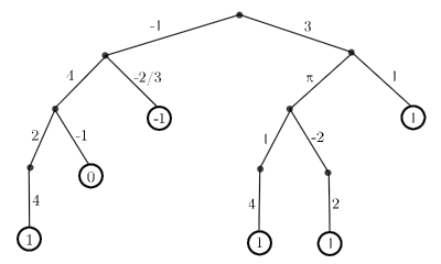
Figure 1: The Schmeling tree corresponding to monomial $\mathfrak{g}$

There are notions of “height” and “depth” associated with such a tree-representation of a transmonomial $\mathfrak{g}$. Let us say that $\mathfrak{g}$ has tree-height $N$ iff the longest branch (from root to leaf) has $N$ edges; and that $\mathfrak{g}$ has tree-depth $M$ iff $M$ is the largest label on a leaf. So the example in Figure 1 has tree-height $4$ and tree-depth $1$. These definitions are convenient for analysis of such a tree diagram. They may differ from the notions of “height” and “depth” defined in [8]. If $\mathfrak{g}$ has height $N$ (that is, $\mathfrak{g}\in\mathfrak{G}_{N\bullet}$), then $\mathfrak{g}$ has tree-height at most $N+1$. But it may be much smaller; for example,

$$\mathfrak{g}=e^{\displaystyle e^{e^{x}}+x}$$

has tree-height $1$ but height $3$. If $\mathfrak{g}$ has depth $M$ (that is, $\mathfrak{g}\in\mathfrak{G}_{\bullet M}$), then $\mathfrak{g}$ has tree-depth $M$ or $M+1$, at least if we have allowed negative values of $M$. The same example $\mathfrak{g}$ has depth $0$ and tree-depth $0$, but

$$\mathfrak{g}=e^{\displaystyle e^{e^{x}}+x^{2}}$$

has depth $0$ and tree-depth $1$.

Tree-height and tree-depth behave in the same way as height and depth under composition on the right by $\log$ or $\exp$. That is: if $\mathfrak{g}$ has tree-height $N$ and tree-depth $M$, then $\mathfrak{g}\circ\exp$ has tree-height $N$ and tree-depth $M-1$, and $\mathfrak{g}\circ\log$ has tree-height $N$ and tree-depth $M+1$. Any $\mathfrak{g}\in\mathfrak{G}_{0}$ has tree-depth $\leq-1$, so $\mathfrak{g}\circ\exp$ has tree-depth $\leq 0$. If tree-depth is $\leq 0$ is it sometimes convenient to extend all branches (using single edges with coefficient $1$) so that all leaves are $x$.

Schmeling Tree and Deriviative

Let $\mathfrak{g}$ be a transmonomial represented as a Schmeling tree. What are the monomials in the support of the derivative $\mathfrak{g}^{\prime}$? Since $\mathfrak{g}=e^{L}$, the derivative is $e^{L}L^{\prime}$, so the monomials in its support have the form $\mathfrak{g}$ times a monomial in the support of $L^{\prime}$. Continuing this recursively, we see that a monomial in $\operatorname{supp}\mathfrak{g}^{\prime}$ looks like

$$\mathfrak{g}\;\mathfrak{g}_{i_{1}}\;\mathfrak{g}_{i_{1}i_{2}}\;\cdots\;\mathfrak{g}_{i_{1}i_{2}\cdots i_{s-1}}\;(\log_{m}x)^{\prime}$$ (1)

where $s$ is chosen so that $\mathfrak{g}_{i_{1}i_{2}\cdots i_{s}}=\log_{m}x$, and of course $(\log_{m}x)^{\prime}$ is itself a monomial. (The monomials $\mathfrak{g}_{i_{1}},\cdots,\mathfrak{g}_{i_{1}i_{2}\cdots i_{s-1}}$ are large, but if $m>0$, then the monomial $(\log_{m}x)^{\prime}$ is small.) So there is one term of $\mathfrak{g}^{\prime}$ for each branch (from root to leaf) of the tree. In the derivative $\mathfrak{g}^{\prime}$, the coefficient for monomial (1) is

$$c_{i_{1}}\;c_{i_{1}i_{2}}\;\cdots\;c_{i_{1}i_{2}\cdots i_{s}},$$

the product of all the edge-labels on the corresponding branch.

Example 3.6.

Following the tree in the example (Figure 1), we may write the derivative $\mathfrak{g}^{\prime}$ with one term for each of the six branches of the tree:

$$\mathfrak{g}^{\prime}=\quad \;(-1)\cdot 4\cdot 2\cdot 4\cdot\mathfrak{g}\mathfrak{g}_{0}\mathfrak{g}_{00}\mathfrak{g}_{000}\cdot(\log x)^{\prime}$$

$$+ \;(-1)\cdot 4\cdot(-1)\cdot\mathfrak{g}\mathfrak{g}_{0}\mathfrak{g}_{00}\cdot x^{\prime}$$

$$+ \;(-1)\cdot(-2/3)\cdot\mathfrak{g}\mathfrak{g}_{0}\cdot(\exp x)^{\prime}$$

$$+ \;3\cdot\pi\cdot 1\cdot 4\cdot\mathfrak{g}\mathfrak{g}_{1}\mathfrak{g}_{10}\mathfrak{g}_{100}\;\cdot(\log x)^{\prime}$$

$$+ \;3\cdot\pi\cdot(-2)\cdot 2\cdot\mathfrak{g}\mathfrak{g}_{1}\mathfrak{g}_{10}\mathfrak{g}_{101}\;\cdot(\log x)^{\prime}$$

$$+ \;3\cdot 1\cdot\mathfrak{g}\mathfrak{g}_{1}\cdot(\log x)^{\prime}.$$

The monomial (1) without the first factor $\mathfrak{g}$ is an element of the set $\operatorname{lsupp}(\mathfrak{g})$. The magnitude of $\mathfrak{g}^{\prime}$ is the monomial we get following the left-most branch

$$\mathfrak{g}\;\mathfrak{g}_{0}\;\mathfrak{g}_{00}\;\cdots\;\mathfrak{g}_{00\cdots 0}\;(\log_{m}x)^{\prime},$$

since all other branches are far smaller.

In the special case where the tree-depth of $\mathfrak{g}$ is $\leq 0$, and we extend all branches so that all leaves are $x$, the monomials in $\mathfrak{g}^{\prime}$ are

$$\mathfrak{g}\;\mathfrak{g}_{i_{1}}\;\mathfrak{g}_{i_{1}i_{2}}\;\cdots\;\mathfrak{g}_{i_{1}i_{2}\cdots i_{s-1}}$$ (0)

where $s$ is chosen with $\mathfrak{g}_{i_{1}i_{2}\cdots i_{s}}=x$. In this case, all monomials $\mathfrak{g}_{i_{1}}\cdots\mathfrak{g}_{i_{1}i_{2}\cdots i_{s-1}}$ in $\operatorname{lsupp}\mathfrak{g}$ are large, and we have

$$\mathfrak{m}:=\max\operatorname{lsupp}\mathfrak{g}=\mathfrak{g}_{0}\mathfrak{g}_{00}\cdots\mathfrak{g}_{00\cdots 0}=\operatorname{mag}(\mathfrak{g}^{\prime}/\mathfrak{g}).$$

Then $\mathfrak{g}^{\prime}\sim\mathfrak{g}\mathfrak{m}$, and we get $\mathfrak{g}^{(n)}\sim\mathfrak{g}\mathfrak{m}^{n}$ for all $n\in\mathbb{N}$ by induction using $\mathfrak{m}^{2}\succ\mathfrak{m}^{\prime}$ [8, Prop. 3.82(iv)]. (This may not hold when $\mathfrak{g}$ has positive tree-depth.)

Proposition 3.7.

Let $T,V\in\mathbb{T}$. Assume all monomials in $T$ have tree-depth $\leq 0$, and $V\prec 1/\mathfrak{m}$ where $\mathfrak{m}=\max\operatorname{lsupp}T$. Then

$$T^{(n)}V^{n},\qquad n\in\mathbb{N}$$

is point-finite, so the series

$$\sum_{n=0}^{\infty}T^{(n)}(x)\frac{V^{n}}{n!}$$

converges in the asymptotic topology.

Proof.

Fix finite set ${\boldsymbol{\mu}}\subset\mathfrak{G}^{\mathrm{small}}$ so that all far-smaller inequalities are witnessed by ${\boldsymbol{\mu}}$: in particular, $V\prec^{{\boldsymbol{\mu}}}1/\mathfrak{m}$ and $T=\operatorname{dom}(T)\cdot(1+S)$ with $S\prec^{{\boldsymbol{\mu}}}1$. Note that $T^{(n+1)}\sim\mathfrak{m}T^{(n)}$. Then

$$T\succ^{{\boldsymbol{\mu}}}T^{\prime}V\succ^{{\boldsymbol{\mu}}}T^{\prime\prime}V^{2}\succ^{{\boldsymbol{\mu}}}\dots,$$

so by [8, Prop. 4.17] the series $\sum T^{(n)}(x)V^{n}/n!$ is point-finite. ∎

Remark 3.8.

The same result should be true for other $T$, perhaps using $\operatorname{tsupp}$ not $\operatorname{lsupp}$; see [9, Def. 7.1].

4 Properties of Composition

Composition $T\circ S$ is defined when $T,S\in\mathbb{T}$ and $S$ is large and positive. As usual we will write $T=T(x)$ and $T\circ S=T(S)$.

Notation 4.1.

Write $\mathcal{P}$ for the group of large positive transseries. And $\SS$ for the subgroup $\SS=x+\mathrm{o}(x)=\left\{\,{T\in\mathbb{T}}:{\operatorname{dom}T=x}\,\right\}=\left\{\,{T\in\mathbb{T}}:{T\sim x}\,\right\}$. For now, think of $\mathcal{P}$ and $\SS$ as sets. They are closed under composition. For existence of inverses: well-based, Proposition 4.20; grid-based, [9, Sec. 8].

Many basic properties of composition may be proved by applying an inductive principle such as Proposition 3.1 to the left composand $T$. (I may—perhaps misleadingly—call this “induction on the height”.) Here are some examples.

Proposition 4.2.

Let $T,T_{1},T_{2}\in\mathbb{T},S\in\mathcal{P}$. Then

$$T>0\Longrightarrow{} T\circ S>0,$$

$$T=0\Longrightarrow{} T\circ S=0,$$

$$T<0\Longrightarrow{} T\circ S<0,$$

$$T_{1}<T_{2}\Longrightarrow{} T_{1}\circ S<T_{2}\circ S,$$

$$T_{1}=T_{2}\Longrightarrow{} T_{1}\circ S=T_{2}\circ S,$$

$$T_{1}>T_{2}\Longrightarrow{} T_{1}\circ S>T_{2}\circ S,$$

$$T\prec 1\Longrightarrow{} T\circ S\prec 1,$$

$$T\succ 1\Longrightarrow{} T\circ S\succ 1,$$

$$T\asymp 1\Longrightarrow{} T\circ S\asymp 1,$$

$$T\sim 1\Longrightarrow{} T\circ S\sim 1,$$

$$T_{1}\prec T_{2}\Longrightarrow{} T_{1}\circ S\prec T_{2}\circ S,$$

$$T_{1}\succ T_{2}\Longrightarrow{} T_{1}\circ S\succ T_{2}\circ S,$$

$$T_{1}\asymp T_{2}\Longrightarrow{} T_{1}\circ S\asymp T_{2}\circ S,$$

$$T_{1}\sim T_{2}\Longrightarrow{} T_{1}\circ S\sim T_{2}\circ S,$$

$$T\circ S\asymp\operatorname{mag}(T\circ S)={} \operatorname{mag}((\operatorname{mag}T)\circ S)\asymp(\operatorname{mag}T)\circ S,$$

$$T\circ S\sim\operatorname{dom}(T\circ S)={} \operatorname{dom}((\operatorname{dom}T)\circ S)\sim(\operatorname{dom}T)\circ S.$$

Some corresponding things may fail for the other composand: Let $T=e^{x}$, $S_{1}=x+\log x$, and $S_{2}=x$. Then $S_{1}\asymp S_{2}$ but $T\circ S_{1}\succ T\circ S_{2}$; $\operatorname{dom}(T\circ S_{1})\not\asymp T\circ\operatorname{dom}S_{1}$.

Proposition 4.3.

Let $S_{1},S_{2}\in\mathcal{P}$, $S_{1}<S_{2}$.

• if $c\in\mathbb{R},c>0$, then $S_{1}^{c}<S_{2}^{c}$,

• if $c\in\mathbb{R},c<0$, then $S_{1}^{c}>S_{2}^{c}$,

• $\log(S_{1})<\log(S_{2})$.

• $\exp(S_{1})<\exp(S_{2})$,

Proof.

(a) Write the canonical multiplicative decomposition $S_{1}=a_{1}e^{L_{1}}(1+U_{1})$ as in 1.3, and similarly $S_{2}=a_{2}e^{L_{2}}(1+U_{2})$. Then

$$S_{1}^{c}=a_{1}^{c}e^{cL_{1}}\left(1+cU_{1}+\sum_{j=2}^{\infty}c_{j}U_{1}^{j}\right),\quad S_{2}^{c}=a_{2}^{c}e^{cL_{2}}\left(1+cU_{2}+\sum_{j=2}^{\infty}c_{j}U_{2}^{j}\right),$$ (1)

for certain (binomial) coefficients $c_{j}$. Now for $S_{1}<S_{2}$ there are these cases: (i) $L_{1}<L_{2}$; (ii) $L_{1}=L_{2},a_{1}<a_{2}$; (iii) $L_{1}=L_{2},a_{1}=a_{2},U_{1}<U_{2}$. But in each of these cases, applying equations (1) shows $S_{1}^{c}<S_{2}^{c}$. For case (iii):

$$S_{2}^{c}-S_{1}^{c}=a_{1}^{c}e^{cL_{1}}(U_{2}-U_{1})\left(c+\sum_{j=2}^{\infty}c_{j}(U_{2}^{j-1}+U_{2}^{j-2}U_{1}+\cdots+U_{1}^{j-1})\right)>0$$

since the terms in the $\sum$ are all ${}\prec 1$.

(b) is similar.

(c) Write canonical multiplicative decomposition $S_{1}=a_{1}e^{L_{1}}(1+U_{1})$ as in 1.3 and similarly $S_{2}=a_{2}e^{L_{2}}(1+U_{2})$. Then

$$\log(S_{1}) =\log(a_{1})+L_{1}+U_{1}+\sum_{j=2}^{\infty}c_{j}U_{1}^{j},$$

$$\log(S_{2}) =\log(a_{2})+L_{2}+U_{2}+\sum_{j=2}^{\infty}c_{j}U_{2}^{j},$$

for certain coefficients $c_{j}$. The same cases (i)—(iii) may be used, and in each case we get $\log(S_{1})<\log(S_{2})$. Case (iii) has reasoning as we did before for (a).

(d) For this, write the canonical additive decomposition $S_{1}=L_{1}+c_{1}+U_{1}$ as in 1.2, and similarly $S_{2}=L_{2}+c_{2}+U_{2}$. Then

$$e^{S_{1}}=e^{c_{1}}e^{L_{1}}\left(1+U_{1}+\sum_{j=2}^{\infty}c_{j}U_{1}^{j}\right),\qquad e^{S_{2}}=e^{c_{2}}e^{L_{2}}\left(1+U_{2}+\sum_{j=2}^{\infty}c_{j}U_{2}^{j}\right),$$

for certain coefficients $c_{j}$. For $S_{1}<S_{2}$ there are three cases: (i) $L_{1}<L_{2}$; (ii) $L_{1}=L_{2},c_{1}<c_{2}$; (iii) $L_{1}=L_{2},c_{1}=c_{2},U_{1}<U_{2}$. In all three cases we get $e^{S_{1}}<e^{S_{2}}$. ∎

Proposition 4.4.

(a) If $T\in\mathbb{T}$, $T>0$, $T\neq 1$, then $\log T<T-1$. (b) If $T\in\mathbb{T}$, $T\neq 0$, then $\exp T>T+1$

Proof.

First note: If $L$ is purely large and positive, then $e^{L}\succ L$. First use [8, Prop. 3.72] for log-free $L$. Then Proposition 4.2 to compose with $\log_{M}$ on the inside. It follows that: If $T\succ 1$ and $T>0$, then $e^{T}\succ T$.

(a) Write $A=\log(T)-T+1$; I must show $A<0$. Write canonical multiplicative decomposition $T=ae^{L}(1+U)$ as in 1.3. Then $\log(T)=\log(a)+L-\sum_{j=1}^{\infty}(-1)^{j}U^{j}/j$. Now if $L>0$, then $T\succ 1$, $T\succ L\succ 1$, so $A\sim-T<0$. If $L<0$, then $T\prec 1\prec L$, so $A\sim L<0$. So assume $L=0$. Now if $a\neq 1$, then $A\sim\log(a)-a+1$, which is $<0$ by the ordinary real Taylor theorem. So assume $a=1$. Then if $U\neq 0$ we have

$$A=-\sum_{j=1}^{\infty}\frac{(-1)^{j}U^{j}}{j}-(1+U)+1=-\frac{U^{2}}{2}+\mathrm{o}(U^{2})<0.$$

So the only case left is $U=0$, and that means $T=1$.

(b) Write $A=\exp T-T-1$; I must show $A>0$. Write canonical additive decomposition $T=L+c+V$ as in 1.2. So $\exp T=e^{L}e^{c}(1+V+\dots)$. If $L>0$, then $T\succ 1$, $e^{T}\succ T\succ 1$, so $A\sim e^{T}>0$. If $L<0$, then $e^{T}\prec 1$, $T\sim L\succ 1$, so $A\sim-L<1$. So assume $L=0$. If $c\neq 0$, then $A\sim e^{c}-c-1$, which is $>0$ by the ordinary real Taylor theorem. So assume $c=0$. Then if $V\neq 0$ we have

$$A=\sum_{j=0}^{\infty}\frac{V^{j}}{j!}-V-1=\frac{V^{2}}{2}+\mathrm{o}(V^{2})>0.$$

So the only case left is $V=0$, and that means $T=0$. ∎

Exponentiality

Associated to each large positive transseries is an integer known as its “exponentiality” [13, Exercise 4.10]. If you compose with $\log$ sufficiently many times on the left, the magnitude is a leaf $\mathfrak{l}_{m}$. The number $p$ in the following result is the exponentiality of $Q$, written $p=\operatorname{expo}Q$.

Proposition 4.5.

Let $Q\in\mathcal{P}$. Then there is $p\in\mathbb{Z}$ and $N\in\mathbb{N}$ so that for all $n\geq N$, $\log_{n}\circ\;Q\circ\exp_{n}\sim\exp_{p}$. Equivalently, $\log_{n}Q\sim\mathfrak{l}_{n-p}$.

Proof.

We will use the basic definition for logarithms. Let $A=ce^{L}(1+U)$ be the canonical multiplicative decomposition. If $A\in\mathcal{P}$, this means $c>0$ and $L$ is purely large and positive. Then $\log A=L+\log c+\sum_{j=1}^{\infty}((-1)^{j+1}/j)U^{j}$. From this we get: If $A,B\in\mathcal{P}$, $A\asymp B$, then $\log A\sim\log B$. Write $\mathcal{R}[p,N]:=\left\{\,{Q\in\mathcal{P}}:{\log_{n}Q\sim\mathfrak{l}_{n-p}\text{ for all }n\geq N}\,\right\}$.

(i) $\mathfrak{l}_{m}\in\mathcal{R}[-m,0]$.

(ii) Let $A=ce^{L}(1+U)\in\mathcal{P}$, then $\operatorname{dom}(\log A)=\operatorname{dom}L$, where also $\operatorname{dom}L\in\mathcal{P}$ and (unless $L$ has height $0$) the height of $\operatorname{dom}L$ is less than the height of $\operatorname{dom}A=ce^{L}$. If $\operatorname{dom}L\in\mathcal{R}[p,N]$ then $A\in\mathcal{R}[p+1,N+1]$.

(iii) Let $A$ have height $0$, so $A\sim c\mathfrak{l}_{m}^{b}$, $c,b\in\mathbb{R}$, $c>0$, $b>0$. Then $\log A\sim b\mathfrak{l}_{m+1}$ and $\log_{2}A\sim\mathfrak{l}_{m+2}$, so $A\in\mathbb{R}[-m,2]$.

These rules cover all $\mathcal{P}$. ∎

Remark 4.6.

Alternate terminology: exponentiality = level. So Proposition 4.5 says that the exponential ordered field $\mathbb{R}\begin{picture}(10.0,8.0)(-2.0,2.0)\put(0.0,0.0){\line(0,1){9.0}} \put(2.0,0.0){\line(0,1){9.0}} \put(4.0,0.0){\line(0,1){9.0}} \put(0.0,0.0){\line(1,0){7.0}} \put(0.0,9.0){\line(1,0){7.0}} \end{picture}x\begin{picture}(9.0,8.0)(0.0,2.0)\put(3.0,0.0){\line(0,1){9.0}} \put(5.0,0.0){\line(0,1){9.0}} \put(7.0,0.0){\line(0,1){9.0}} \put(0.0,0.0){\line(1,0){7.0}} \put(0.0,9.0){\line(1,0){7.0}} \end{picture}$ is levelled.

Example 4.7.

$$T\sim 4(\log x)^{2}x^{\pi}e^{5x^{2}-x}$$

(so that the dominant term of $T$ is $4(\log x)^{2}x^{\pi}e^{5x^{2}-x}$), then

$$\log\circ\;T\circ\exp \sim 5e^{2x}-e^{x}+\pi x+2\log x+\log 4\sim 5e^{2x},$$

$$\log_{2}\circ\;T\circ\exp_{2} \sim 2e^{x}+\log 5\sim 2e^{x},$$

$$\log_{3}\circ\;T\circ\exp_{3} \sim e^{x}+\log 2\sim e^{x},$$

$$\log_{k}\circ\;T\circ\exp_{k} \sim e^{x},\qquad\qquad\text{for all }k\geq 3,$$

so $\operatorname{expo}T=1$.

Proposition 4.8.

If $\operatorname{expo}T=0$, then $\log_{k}\circ\;T\circ\exp_{k}$ is log-free for $k$ large enough.

Proof.

Prove recursively: Assume $T=x+A$, $A\in\mathbb{R}\begin{picture}(8.0,8.0)(-2.0,2.0)\put(0.0,0.0){\line(0,1){9.0}} \put(2.0,0.0){\line(0,1){9.0}} \put(0.0,0.0){\line(1,0){5.0}} \put(0.0,9.0){\line(1,0){5.0}} \end{picture}\mathfrak{G}_{\bullet,M}\begin{picture}(7.0,8.0)(0.0,2.0)\put(3.0,0.0){\line(0,1){9.0}} \put(5.0,0.0){\line(0,1){9.0}} \put(0.0,0.0){\line(1,0){5.0}} \put(0.0,9.0){\line(1,0){5.0}} \end{picture}$, $M>0$, $A\prec x$. Then $T\circ\exp=e^{x}+A\circ\exp=e^{x}(1+B)$ with $B=(A/x)\circ\exp\in\mathbb{R}\begin{picture}(8.0,8.0)(-2.0,2.0)\put(0.0,0.0){\line(0,1){9.0}} \put(2.0,0.0){\line(0,1){9.0}} \put(0.0,0.0){\line(1,0){5.0}} \put(0.0,9.0){\line(1,0){5.0}} \end{picture}\mathfrak{G}_{\bullet,M-1}\begin{picture}(7.0,8.0)(0.0,2.0)\put(3.0,0.0){\line(0,1){9.0}} \put(5.0,0.0){\line(0,1){9.0}} \put(0.0,0.0){\line(1,0){5.0}} \put(0.0,9.0){\line(1,0){5.0}} \end{picture}$ and $\log\circ\;T\circ\exp=x+\sum_{j=1}^{\infty}(-1)^{j+1}B^{j}/j$ has depth $M-1$. ∎

Simpler Proof Needed

Here is a simple fact. It needs a simple proof. It is true for functions, so it is surely true for transseries as well. My overly-involved proof will be given in Section 8. In fact, there are two propositions. Each can be deduced from the other:

Proposition 4.9.

Let $T\in\mathbb{T}$, $S_{1},S_{2}\in\mathcal{P}$, $S_{1}<S_{2}$. Then

$$T^{\prime}>0\Longrightarrow{} T\circ S_{1}<T\circ S_{2},$$

$$T^{\prime}=0\Longrightarrow{} T\circ S_{1}=T\circ S_{2},$$ (1)

$$T^{\prime}<0\Longrightarrow{} T\circ S_{1}>T\circ S_{2}.$$

Proposition 4.10.

Let $A,B\in\mathbb{T}$, $S_{1},S_{2}\in\mathcal{P}$, $A^{\prime}\prec B^{\prime}$, $S_{1}<S_{2}$. Then

$$A\circ S_{2}-A\circ S_{1}\prec B\circ S_{2}-B\circ S_{1}.$$ (2)

Proof of 4.10 from 4.9.

Since the theorem is unchanged when we replace $B$ by $-B$, we may assume $B^{\prime}>0$. We have $A^{\prime}\prec B^{\prime}$. Let $c\in\mathbb{R}$. By Remark 1.6, $B^{\prime}>cA^{\prime}$ so $(B-cA)^{\prime}>0$. Therefore, by Proposition 4.9, $(B-cA)\circ S_{1}<(B-cA)\circ S_{2}$ so

$$B\circ S_{2}-B\circ S_{1}>c\big{(}A\circ S_{2}-A\circ S_{1}\big{)}.$$

This is true for all $c\in\mathbb{R}$, so we have $B\circ S_{2}-B\circ S_{1}\succ A\circ S_{2}-A\circ S_{1}$. ∎

Proof of 4.9 from 4.10.

Let $\mathcal{R}$ be the set of all $T\in\mathbb{T}$ that satisfy (1) for all $S_{1},S_{2}\in\mathcal{P}$ with $S_{1}<S_{2}$. We claim $\mathcal{R}$ satisfies the conditions of Corollary 3.3. Clearly $1,x\in\mathcal{R}$.

(b^′′) Note $\mathfrak{l}_{m}^{\prime}=1/\prod_{j=0}^{m-1}\mathfrak{l}_{j}>0$. If $S_{1}<S_{2}$, then by Proposition 4.3(c) we have $\log_{m}S_{1}<\log_{m}S_{2}$.

(d^′′) Assume $\operatorname{supp}T\subseteq\mathcal{R}$. If $T=0$, the conclusion is clear. Assume $T\neq 0$. Let $a\mathfrak{g}=\operatorname{dom}T$, $a\in\mathbb{R}$, $\mathfrak{g}\in\mathfrak{G}$. We may assume $\mathfrak{g}\neq 1$, since if $\mathfrak{g}=1$, we may consider $T-a\mathfrak{g}$ instead. So $T^{\prime}\sim a\mathfrak{g}^{\prime}$. Write $A=T-a\mathfrak{g}$ so that $T=a\mathfrak{g}+A$ with $A\prec a\mathfrak{g}$. There will be cases based on the signs of $a$ and $\mathfrak{g}^{\prime}$. Take the case $a>0,\mathfrak{g}^{\prime}>0$. So $\mathfrak{g}\circ S_{1}<\mathfrak{g}\circ S_{2}$ since $\mathfrak{g}\in\mathcal{R}$. Now by Proposition 4.10,

$$a\mathfrak{g}\circ S_{2}-a\mathfrak{g}\circ S_{1}\succ A\circ S_{2}-A\circ S_{1},$$

so $T\circ S_{2}-T\circ S_{1}\sim a\mathfrak{g}\circ S_{2}-a\mathfrak{g}\circ S_{1}>0$ and therefore $T\circ S_{2}-T\circ S_{1}>0$. The other three cases are similar.

(e^′′) Let $T=e^{L}$, where $L\in\mathcal{R}$ is purely large. Then $T^{\prime}=L^{\prime}e^{L}$, so $T^{\prime}$ has the same sign as $L^{\prime}$. Thus $L\circ S_{1}<L\circ S_{2}$ if $T^{\prime}>0$ and reversed if $T^{\prime}<0$. Apply Proposition 4.3(d) to get $e^{L\circ S_{1}}<e^{L\circ S_{2}}$ or reversed, as required. ∎

Remark 4.11.

To prove either 4.10 or 4.9 outright seems to require more work than the proofs found above. See Theorem 8.14.

Here is a special case of Proposition 4.10.

Proposition 4.12.

If $A\in\mathbb{T},S_{1},S_{2}\in\mathcal{P}$, $S_{1}<S_{2}$, and $A\prec x$, then $A\circ S_{2}-A\circ S_{1}\prec S_{2}-S_{1}$.

Proof.

Note $A^{\prime}\prec x^{\prime}$ and apply Proposition 4.10. ∎

Grid-Based Version

As we know, $T\prec S$ if and only if $T\prec^{\boldsymbol{\mu}}S$ for some finite set ${\boldsymbol{\mu}}\subset\mathfrak{G}^{\mathrm{small}}$ of generators. So of course Proposition 4.12 needs a form in terms of ratio sets. It is found in [9, Rem. 9.3]:

Proposition 4.13.

Let ${\boldsymbol{\mu}}$ be a ratio set. Let $S_{1},S_{2}\in\mathcal{P}$. Then there is a ratio set ${\boldsymbol{\alpha}}$ such that: For every $A\in\mathbb{T}^{\boldsymbol{\mu}}$, if $A\prec^{\boldsymbol{\mu}}x$, then $A(S_{2})-A(S_{1})\prec^{\boldsymbol{\alpha}}S_{2}-S_{1}$.

Note that ${\boldsymbol{\alpha}}$ depends on $S_{1}$ and $S_{2}$, not just on a ratio set generating them. It is apparently not possible to avoid this problem:

Question 4.14.

Given a ratio set ${\boldsymbol{\mu}}\subset\mathfrak{G}^{\mathrm{small}}$, is there ${\boldsymbol{\alpha}}\supseteq{\boldsymbol{\mu}}$ such that: if $A,S_{1},S_{2}\in\mathbb{T}^{{\boldsymbol{\mu}}}$, $A\prec^{{\boldsymbol{\mu}}}x$, $S_{1},S_{2}\in\mathcal{P}$, and $S_{1}<S_{2}$, then $A\circ S_{2}-A\circ S_{1}\prec^{{\boldsymbol{\alpha}}}S_{2}-S_{1}$?

Example 4.15.

Let ${\boldsymbol{\mu}}=\{x^{-1},e^{-x^{3}}\}$. Consider $A=\mu_{2}=e^{-x^{3}}$ and $S_{a}=\mu_{1}^{-1}+a\mu_{1}=x+ax^{-1}$ for $a\in\mathbb{R}$. Certainly $A\prec^{\boldsymbol{\mu}}1$. Compute

$$A\circ S_{a} =e^{-(x+ax^{-1})^{3}}=e^{-x^{3}-3ax-3a^{2}x^{-1}-a^{3}x^{-3}}$$

$$=e^{-x^{3}-3ax}\left(\sum_{j=0}^{\infty}\frac{(-3a^{2}x^{-1}-a^{3}x^{-3})^{j}}{j!}\right).$$

The dominant term is the monomial $e^{-x^{3}-3ax}$. As $a$ ranges over $\mathbb{R}$, these monomials do not lie in any grid. Nor even in any well ordered set.

Now if $a<b$, then $S_{a}<S_{b}$ and $e^{-x^{3}-3ax}\succ e^{-x^{3}-3bx}$, so

$$S_{b}-S_{a}=(b-a)x^{-1},\qquad A\circ S_{b}-A\circ S_{a}\sim-e^{-x^{3}-3ax}.$$

Of course $A\circ S_{b}-A\circ S_{a}\prec S_{b}-S_{a}$. But there is no finite ${\boldsymbol{\alpha}}$ such that $A\circ S_{b}-A\circ S_{a}\prec^{{\boldsymbol{\alpha}}}S_{b}-S_{a}$ for all $a,b$ ranging over the reals.

Integral Notation

Notation 4.16.

If $A,B\in\mathbb{T}$ and $A^{\prime}=B$, we may sometimes write $A=\int B$, but in fact $A$ is only determined by $B$ up to a constant summand. The large part of $A$ is determined by $B$. We also write $\int_{S_{1}}^{S_{2}}B:=A(S_{2})-A(S_{1})$, which is uniquely determined by $B$, and is defined for $S_{1},S_{2}\in\mathcal{P},S_{1}<S_{2}$.

Of course, with this definition, any statement about integrals is equivalent to a statement about derivatives. Propositions 4.9 or 4.10 lead to the following.

Corollary 4.17.

Let $A,B\in\mathbb{T}$, $S_{1},S_{2}\in\mathcal{P}$, $S_{1}<S_{2}$. Then

$$B>0\Longrightarrow{} \int_{S_{1}}^{S_{2}}B>0,$$

$$B=0\Longrightarrow{} \int_{S_{1}}^{S_{2}}B=0,$$

$$B<0\Longrightarrow{} \int_{S_{1}}^{S_{2}}B<0.$$

$$A>B\Longrightarrow{} \int_{S_{1}}^{S_{2}}A>\int_{S_{1}}^{S_{2}}B,$$

$$A=B\Longrightarrow{} \int_{S_{1}}^{S_{2}}A=\int_{S_{1}}^{S_{2}}B,$$

$$A<B\Longrightarrow{} \int_{S_{1}}^{S_{2}}A<\int_{S_{1}}^{S_{2}}B.$$

Remark 1.6 lets us prove formulas about $\prec$ from formulas about $<$. Here are some examples.

Proposition 4.18.

If $A,B\in\mathbb{T}$, $A,B$ nonzero, $S_{1},S_{2}\in\mathcal{P}$, $S_{1}<S_{2}$, then

$$A\succ B\Longrightarrow{} \int_{S_{1}}^{S_{2}}A\succ\int_{S_{1}}^{S_{2}}B,$$

$$A\prec B\Longrightarrow{} \int_{S_{1}}^{S_{2}}A\prec\int_{S_{1}}^{S_{2}}B,$$

$$A\asymp B\Longrightarrow{} \int_{S_{1}}^{S_{2}}A\asymp\int_{S_{1}}^{S_{2}}B,$$

$$A\sim B\Longrightarrow{} \int_{S_{1}}^{S_{2}}A\sim\int_{S_{1}}^{S_{2}}B.$$

Compositional Inverse

Now using Proposition 4.12 we get a nice proof for the existence of inverses under composition. (For the well-based case.) See also [7, Cor. 6.25].

Proposition 4.19.

Let $T=x+A$, $A\prec x$, $\operatorname{supp}A\subset\mathfrak{G}_{N}$. Then $T$ has an inverse $S$ under composition, $S=x+B$, $B\prec x$, $\operatorname{supp}B\subset\mathfrak{G}_{N}$.

Proof.

Let the function $\Phi$ be defined by $\Phi(S)=x-A\circ S$. Then $\Phi$ maps $\mathcal{A}:=\left\{\,{x+B}:{B\prec x,\operatorname{supp}B\subseteq\mathfrak{G}_{N}}\,\right\}$ into itself [8, Prop. 3.98]. I claim $\Phi$ is contracting on $\mathcal{A}$. Indeed, if $S_{1},S_{2}\in\SS$ and $S_{1}\neq S_{2}$, then

$$\Phi(S_{2})-\Phi(S_{1})=A\circ S_{1}-A\circ S_{2}\prec S_{2}-S_{1}$$

by Proposition 4.12.

Apply the fixed-point theorem [12, Thm. 4.7] (see Proposition 6.4, below) to get $S$ with $S=\Phi(S)$. Then

$$T\circ S=S+A\circ S=\Phi(S)+A\circ S=x.$$

As is well-known: if right inverses all exist, then they are full inverses. Review of the proof: Suppose $T\circ S=x$ as found. Start with $S$ and get a right-inverse $T_{1}$ so $S\circ T_{1}=x$. Then $T=T\circ x=T\circ(S\circ T_{1})=(T\circ S)\circ T_{1}=x\circ T_{1}=T_{1}$. ∎

Proposition 4.20.

The set $\mathcal{P}$ is a group under composition.

Proof.

Let $T\in\mathcal{P}$. Let $p=\operatorname{expo}T$, so that $\log_{k}\circ T\circ\exp_{k}\sim\exp_{p}$ for large enough $k$. Let $T_{1}=\log_{k}\circ T\circ\exp_{k-p}$, so that $T_{1}\sim x$ and (if $k$ is large enough) $T_{1}$ is log-free. By Proposition 4.19 there is an inverse, say $T_{1}\circ S_{1}=x$. Write $S=\exp_{k-p}S_{1}\circ\log_{k}$. Then $T\circ S=\exp_{k}\circ T_{1}\circ\log_{k-p}\circ\exp_{k-p}\circ S_{1}\circ\log_{k}=x$. ∎

Remark 4.21.

We need a grid-based version of Proposition 4.12 to prove existence of a grid-based compositional inverse using a grid-based fixed-point theorem. This is done in [9, Sec. 8].

An Example Inverse

Consider the transseries $S=\log x+1+x^{-1}\in\mathcal{P}$. We want to discuss its compositional inverse. According to the method above, we should compute the inverse of $S_{1}=S\circ\exp=x+1+e^{-x}\in\mathcal{P}$. And if $T_{1}=S_{1}^{[-1]}$, then $S^{[-1]}=\exp\circ T_{1}$.

For the inverse of $S_{1}=x+1+e^{-x}$, write $A=1+e^{-x}$ and solve by iteration $Y=\Phi(Y)$, where $\Phi(Y)=x-A\circ Y=x-1-e^{-Y}$. We end up with

$$T_{1} =x-1-ee^{-x}-e^{2}e^{-2x}-\frac{3e^{3}}{2}e^{-3x}-\frac{8e^{4}}{3}e^{-4x}+\cdots$$

$$=x-1-\sum_{j=1}^{\infty}a_{j}e^{-jx}$$

either by iteration, or with a linear equation for each $a_{j}$ in terms of the previous ones. (And $a_{j}$ is rational times $e^{j}$.) And then

$$S^{[-1]} =e^{T_{1}}=\frac{1}{e}e^{x}-1-\frac{e}{2}e^{-x}-\frac{2e^{2}}{3}e^{-2x}-\frac{9e^{3}}{8}e^{-3x}-\frac{32e^{4}}{15}e^{-4x}+\cdots$$

$$=\frac{1}{e}e^{x}-1-\sum_{j=1}^{\infty}b_{j}e^{-jx}.$$

Compositional Equations

Because of the group property Proposition 4.20 (or the grid-based version [9, Sec. 8]), we know: Let $S,T\in\mathbb{T}$. If $S,T$ are both large and positive, then there is a unique $Y\in\mathcal{P}$ with $S=T\circ Y$.

Proposition 4.22.

Let $S,T\in\mathbb{T}$. Then there is a unique $Y\in\mathcal{P}$ with $S=T\circ Y$ in each of the following cases: $S$ and $T$ are both:

• large and positive

• small and positive

• large and negative

• small and negative

• For some $c\in\mathbb{R}$, $c\neq 0$, $S\sim c$, $T\sim c$, $S>c$, $T>c$.

• For some $c\in\mathbb{R}$, $c\neq 0$, $S\sim c$, $T\sim c$, $S<c$, $T<c$.

There is a nonunique $Y\in\mathcal{P}$ with $S=T\circ Y$ in case: for some $c\in\mathbb{R}$, both $S=c$ and $T=c$. In all other cases, there is no $Y$ with $S=T\circ Y$.

Proof.

(a) is from Proposition 4.20. (b) Apply (a) to $1/S$ and $1/T$. (c) Apply (a) to $-S$ and $-T$. (d) Apply (b) to $-S$ and $-T$. (e) Apply (b) to $S-c$ and $T-c$. (f) Apply (d) to $S-c$ and $T-c$.

The concluding cases are clear. ∎

Mean Value Theorem

Using Proposition 4.9, we get a MVT.

Proposition 4.23.

Given $A\in\mathbb{T},S_{1},S_{2}\in\mathcal{P}$, $S_{1}<S_{2}$, there is $S\in\mathcal{P}$ so that

$$\frac{A\circ S_{2}-A\circ S_{1}}{S_{2}-S_{1}}=A^{\prime}\circ S.$$

Proof.

Write $B=(A\circ S_{2}-A\circ S_{1})/(S_{2}-S_{1})$. We claim that Proposition 4.22 shows that there is a solution $S$ to $B=A^{\prime}\circ S$. So we have to show that $A^{\prime},B$ are in the same case of Proposition 4.22.

Let $c\in\mathbb{R}$. If $A^{\prime}>c$, then $(A-cx)^{\prime}>0$, and therefore by Proposition 4.9 $(A-cx)\circ S_{1}<(A-cx)\circ S_{2}$, so $A\circ S_{2}-A\circ S_{1}>c(S_{2}-S_{1})$, so $(A\circ S_{2}-A\circ S_{1})/(S_{2}-S_{1})>c$, so $B>c$. Similarly: if $A^{\prime}<c$, then $B<c$. These hold for all real $c$, so in fact $A^{\prime}$ and $B$ are in the same case. ∎

The following proposition, too, has—so far—only an involved proof, which will not be given here. See Section 5 for this and still more versions of the Mean Value Theorem.

Proposition 4.24.

Let $A\in\mathbb{T},S_{1},S_{2}\in\mathcal{P}$. If $A^{\prime\prime}>0$ and $S_{1}<S_{2}$, then

$$A^{\prime}\circ S_{1}<\frac{A\circ S_{2}-A\circ S_{1}}{S_{2}-S_{1}}<A^{\prime}\circ S_{2}.$$

Using this, we can improve the Mean Value Theorem 4.23:

Proposition 4.25.

Given $A\in\mathbb{T},S_{1},S_{2}\in\mathcal{P}$, $S_{1}<S_{2}$, there is $S\in\mathcal{P}$, $S_{1}<S<S_{2}$ so that

$$\frac{A\circ S_{2}-A\circ S_{1}}{S_{2}-S_{1}}=A^{\prime}\circ S.$$

Proof.

First assume $A^{\prime\prime}>0$. Let $S$ be as in Proposition 4.23. By Proposition 4.24, $A^{\prime}(S_{1})<A^{\prime}(S)<A^{\prime}(S_{2})$. So by Proposition 4.9 we conclude $S_{1}<S<S_{2}$.

The case $A^{\prime\prime}<0$ is similar. The case $A^{\prime\prime}=0$ is easy. ∎

Intermediate Value Theorem

Proposition 4.26.

Let $K,T\in\mathbb{T}$, $A,B\in\mathcal{P}$. Assume $T(A)\leq K\leq T(B)$. Then there is $S\in\mathcal{P}$ with $T(S)=K$ and either $A\leq S\leq B$ or $A\geq S\geq B$.

Proof.

If $T(A)=K$, choose $S=A$; if $T(B)=K$, choose $S=B$. So we may assume $T(A)<K<T(B)$. We will consider cases for $T$.

(a) First assume $T$ is large and positive. Then the inverse $T^{[-1]}$ exists in $\mathcal{P}$. Also $T(A),T(B)$ are large and positive, so $K$, which is between them, is large and positive. Define $S=T^{[-1]}(K)$. Of course $T(S)=K$. Since $T^{[-1]}$ is large and positive it is increasing (by Proposition 4.9), so applying $T^{[-1]}$ to $T(A)<K<T(B)$ we get $A<S<B$.

(b) Assume $T$ is large and negative. Apply case (a) to $-T$.

(c) Assume $T$ is small and positive. Apply case (a) to $1/T$.

(d) Assume $T$ is small and negative. Apply case (c) to $-T$.

(e) Assume there is $a\in\mathbb{R}$ with $T\sim a,T>a$. Apply case (c) to $T-a$.

(f) Assume there is $a\in\mathbb{R}$ with $T\sim a,T<a$. Apply case (d) to $T-a$.

(g) The only case left is $T=a$ for some $a\in\mathbb{R}$, so $T(A)=T(B)=a=K$, and this case was taken care of at the beginning of the proof. Or let $S=(A+B)/2$ to get $S$ strictly between $A$ and $B$ when $A\neq B$. ∎

Remark 4.27.

Using 4.26 we can deduce 4.25 from 4.24 without the need of 4.23. But 4.24 is still the difficult step.

5 Taylor’s Theorem

Here we will formulate many versions of Taylor’s Theorem. Unfortunately, proofs are (as far as I know) still quite involved. Proofs (for most cases) will not be included here. See [7, §6] for well-based transseries and [13, §5.3] for grid-based transseries. But in some cases it may not be clear that they have proved everything listed here.

Recall definitions $\mathfrak{G}_{N}$, $\mathfrak{G}_{N,M}$, $\mathfrak{G}_{\bullet}$, etc. If $\mathfrak{A}$ is a set of monomials, and $S\in\mathcal{P}$, write $\mathfrak{A}\circ S:=\left\{\,{\mathfrak{g}\circ S}:{\mathfrak{g}\in\mathfrak{A}}\,\right\}$. Let $U\in\mathbb{T}$, then we say $U\prec\mathfrak{A}$ if $U\prec\mathfrak{g}$ for all $\mathfrak{g}\in\mathfrak{A}$. Recall that if $\mathfrak{g}\in\mathfrak{G}_{N,M}\setminus\mathfrak{G}_{N-1,M}$ and $\mathfrak{g}\prec 1$, then $\mathfrak{g}\prec\mathfrak{G}_{N-1,M}$.

Let $T\in\mathbb{T}$, $S_{1},S_{2}\in\mathcal{P}$. For $n\in\mathbb{N}$ define

$$\Delta_{n}(T,S_{1},S_{2}):=T(S_{2})-\sum_{k=0}^{n-1}\frac{T^{(k)}(S_{1})}{k!}\,(S_{2}-S_{1})^{k}.$$

When $S_{1},S_{2}$ are understood, write $\Delta_{n}(T)$. The first few cases:

$$\Delta_{0}(T) =T(S_{2}),$$

$$\Delta_{1}(T) =T(S_{2})-T(S_{1}),$$

$$\Delta_{2}(T) =T(S_{2})-T(S_{1})-T^{\prime}(S_{1})\cdot(S_{2}-S_{1}),$$

$$\Delta_{3}(T) =T(S_{2})-T(S_{1})-T^{\prime}(S_{1})\cdot(S_{2}-S_{1})-\frac{1}{2}T^{\prime\prime}(S_{1})\cdot(S_{2}-S_{1})^{2}.$$

Note that derivatives $\partial^{k}$ are strongly additive, and therefore these $\Delta_{n}$ are also. That is: if $S=\sum_{i\in I}A_{i}$ (in the asymptotic topology), then $\Delta_{n}(S)=\sum\Delta_{n}(A_{i})$.

Notation 5.1.

Formulations.

• Let $T\in\mathbb{T}_{N,M}$, $T\notin\mathbb{R}$, $S_{1},S_{2}\in\mathcal{P}$. If $N=0$ assume $S_{2}-S_{1}\prec S_{1}$. If $N>0$ assume $S_{2}-S_{1}\prec\mathfrak{G}_{N-1,M}\circ S_{1}$. Let $n\in\mathbb{N}$. If $T^{(n)}\neq 0$, then

  $$\Delta_{n}(T)\sim\frac{T^{(n)}(S_{1})}{n!}\,(S_{2}-S_{1})^{n}.$$

• Let $T\in\mathbb{T}_{N,M}$, $T\notin\mathbb{R}$, $S_{1},S_{2}\in\mathcal{P}$. If $N=0$ assume $S_{2}-S_{1}\prec S_{1}$. If $N>0$ assume $S_{2}-S_{1}\prec\mathfrak{G}_{N-1,M}\circ S_{1}$. Then

  $$T(S_{2})=\sum_{j=0}^{\infty}\frac{T^{(j)}(S_{1})}{j!}\,(S_{2}-S_{1})^{j}.$$

• Let $T\in\mathbb{T}$, let $S_{1},S_{2}\in\mathcal{P}$, and let $n\in\mathbb{N}$. If $T^{(n+1)}>0$ and $S_{1}<S_{2}$, then

  $$\frac{T^{(n)}(S_{1})}{n!}\,(S_{2}-S_{1})^{n}<\Delta_{n}(T)<\frac{T^{(n)}(S_{2})}{n!}\,(S_{2}-S_{1})^{n}.$$

  Other cases also: If $T^{(n+1)}<0$, reverse the inequalities. If $S_{1}>S_{2}$ and $n$ is even, reverse the inequalities.

• Let $T\in\mathbb{T}$, let $S_{1},S_{2}\in\mathcal{P}$, and let $n\in\mathbb{N}$. If $T^{(n)}>0$ and $S_{1}<S_{2}$, then $\Delta_{n}(T)>0$. Other cases also: If $T^{(n)}<0$, reverse the inequality. If $S_{1}>S_{2}$ and $n$ is odd, reverse the inequality.

• Let $A,B\in\mathbb{T}$, let $S_{1},S_{2}\in\mathcal{P}$, and let $n\in\mathbb{N}$. If $A^{(n)}\prec B^{(n)}$ then $\Delta_{n}(A)\prec\Delta_{n}(B)$.

Some beginning cases.

• If $(S_{2}-S_{1})$ is appropriately small, then $T(S_{2})\sim T(S_{1})$.

• If $(S_{2}-S_{1})$ is appropriately small, then $T(S_{2})-T(S_{1})\sim T^{\prime}(S_{1})\cdot(S_{2}-S_{1})$. Proved in 7.1.

• If $T^{\prime}>0$ and $S_{1}<S_{2}$, then $T(S_{1})<T(S_{2})<T(S_{2})$. (Second inequality is too strong.) This is 4.9, proved in 8.14.

• If $T^{\prime\prime}>0$ and $S_{1}\neq S_{2}$, then

  $$T^{\prime}(S_{1})<\frac{T(S_{2})-T(S_{1})}{S_{2}-S_{1}}<T^{\prime}(S_{2}).$$

  This is 4.24.

• If $T>0$, then $T(S_{2})>0$. This is in 4.2.

• If $T^{\prime}>0$ and $S_{1}<S_{2}$, then $T(S_{2})-T(S_{1})>0$. This is 4.9 again.

• If $A\prec B$ then $A(S_{2})\prec B(S_{2})$. This is in 4.2.

• If $A^{\prime}\prec B^{\prime}$ then $A(S_{2})-A(S_{1})\prec B(S_{2})-B(S_{1})$. This is 4.10, proof in 8.14.

A variant form of [$\mathbf{B}_{n}$] follows using the intermediate value theorem (a consequence of [$\mathbf{B}_{1}$]).

• Let $T\in\mathbb{T}$, let $S_{1},S_{2}\in\mathcal{P}$, and let $n\in\mathbb{N}$. If $S_{1}\neq S_{2}$, then there exists $\widetilde{S}$ strictly between $S_{1}$ and $S_{2}$ such that

  $$\Delta_{n}(T,S_{1},S_{2})=\frac{T^{(n)}\big{(}\widetilde{S}\big{)}}{n!}\,(S_{2}-S_{1})^{n}.$$

Good Proofs Needed—But What Methods?

A good exposition is needed for the proofs of the principles stated in 5.1. First steps are seen below (Section 7 for $[\mathbf{A}_{1}]$ and Section 8 for $[\mathbf{C}_{1}]$ and $[\mathbf{D}_{1}]$). Now proofs for $[\mathbf{A}_{n}]$ and $[\mathbf{A}_{\infty}]$ should be possible along the same lines. But I think further proofs for $[\mathbf{B}_{n}],[\mathbf{C}_{n}],[\mathbf{D}_{n}]$ along those lines will be ugly or impossible. So a better approach is needed. Even if proofs can, indeed, be found in the literature (such as [7, §6] and [13, §5.3]), they are not as elementary as one might hope.

Related results could be expected from the same methods, perhaps. For example, does the following follow from the principles listed above, or would it require additional proof?

Let $U,V\in\mathbb{T}$, $S_{1},S_{2}\in\mathcal{P}$. If $U^{\prime}>0,V>0,S_{1}<S_{2}$, then

$$U(S_{1})\int_{S_{1}}^{S_{2}}V<\int_{S_{1}}^{S_{2}}UV<U(S_{2})\int_{S_{1}}^{S_{2}}V.$$

Or: There exists $\widetilde{S}$ between $S_{1}$ and $S_{2}$ with

$$\int_{S_{1}}^{S_{2}}UV=U\big{(}\widetilde{S}\,\big{)}\int_{S_{1}}^{S_{2}}V.$$

Equivalently: Let $A,B\in\mathbb{T},S_{1},S_{2}\in\mathcal{P}$ with $B^{\prime}\neq 0$ and $S_{1}\neq S_{2}$. Then there exists $\widetilde{S}$ between $S_{1}$ and $S_{2}$ with

$$\frac{A(S_{2})-A(S_{1})}{B(S_{2})-B(S_{1})}=\frac{A^{\prime}\big{(}\widetilde{S}\,\big{)}}{B^{\prime}\big{(}\widetilde{S}\,\big{)}}.$$

[Equivalence comes from writing $B^{\prime}=V$, $A^{\prime}=UV$.]

One method used for proofs such as these (in conventional calculus) suggests that we need to know about transseries of two variables in order to use the same proofs in this setting. This remains to be properly defined and investigated.

6 Topology and Convergence

In [8, Def. 3.45] we defined only the “asymptotic topology” for $\mathbb{T}$. But there are other topologies or types of convergence. And none of them has all of the desirable properties.

The attractive topology is described by van der Hoeven [12]; I will use letter H for it, $T_{\gamma}\,\raisebox{1.72218pt}{$\underset{{}^{{}^{\mathrm{H}}}}{\longrightarrow}$}\,T$. For our situation (with totally ordered valuation group $\mathfrak{G}$) it is also the order topology for $\mathbb{T}$ and the topology arising from the valuation $\operatorname{mag}$.

Definition 6.1.

Let $T_{\gamma}$ be a net in $\mathbb{T}$ and let $T\in\mathbb{T}$. Then $T_{\gamma}\,\raisebox{1.72218pt}{$\underset{{}^{{}^{\mathrm{H}}}}{\longrightarrow}$}\,T$ iff for every $\mathfrak{m}\in\mathfrak{G}$ there is $\gamma_{\mathfrak{m}}$ such that for all $\gamma\geq\gamma_{\mathfrak{m}}$ we have $T-T_{\gamma}\prec\mathfrak{m}$.

This is the convergence of a metric. Because every transseries has finite height, there is a countable base for the H-neighborhoods of zero made up of the sets

$$\mathrm{o}(1/\exp_{m})=\left\{\,{T\in\mathbb{T}}:{T\prec 1/\exp_{m}}\,\right\}\qquad\text{for $m=0,1,2,\cdots$}.$$

Here, as usual, $\exp_{0}=x,\exp_{1}=e^{x},\exp_{2}=e^{e^{x}}$, and so on.

Continuity: (The “$\varepsilon$–$\delta$” type definition.) A function $\Psi\colon\mathbb{T}\to\mathbb{T}$ is H-continuous at $S_{0}\in\mathbb{T}$ iff: for every $\mathfrak{m}\in\mathfrak{G}$ there is $\mathfrak{n}\in\mathfrak{G}$ so that for all $S\in\mathbb{T}$, if $S-S_{0}\prec\mathfrak{n}$ then $\Psi(S)-\Psi(S_{0})\prec\mathfrak{m}$. We may write it like this: $\Psi\big{(}S_{0}+\mathrm{o}(\mathfrak{n})\big{)}\subseteq\Psi(S_{0})+\mathrm{o}(\mathfrak{m})$.

The asymptotic topology I get from Costin [3]; I will use letter C for it, $T_{j}\,\raisebox{1.72218pt}{$\underset{{}^{{}^{\mathrm{C}}}}{\longrightarrow}$}\,T$. Recall the definition:

Definition 6.2.

$T_{j}\overset{{\boldsymbol{\mu}},\mathbf{m}}{\longrightarrow}T$ iff $\operatorname{supp}(T_{j})\subseteq\mathfrak{J}^{{\boldsymbol{\mu}},\mathbf{m}}$ for all $j$ and $\operatorname{supp}(T_{j}-T)$ is point-finite;

$T_{j}\overset{{\boldsymbol{\mu}}}{\longrightarrow}T$ iff there exists $\mathbf{m}$ with $T_{j}\overset{{\boldsymbol{\mu}},\mathbf{m}}{\longrightarrow}T$;

$T_{j}\,\raisebox{1.72218pt}{$\underset{{}^{{}^{\mathrm{C}}}}{\longrightarrow}$}\,T$ iff there exists ${\boldsymbol{\mu}}$ with $T_{j}\overset{{\boldsymbol{\mu}}}{\longrightarrow}T$;

Sets $\mathbb{T}^{{\boldsymbol{\mu}},\mathbf{m}}=\left\{\,{T\in\mathbb{T}}:{\operatorname{supp}T\subseteq\mathfrak{J}^{{\boldsymbol{\mu}},\mathbf{m}}}\,\right\}$ are metrizable for  $\underset{{}^{{}^{\mathrm{C}}}}{\longrightarrow}$ . The asymptotic topology for all of $\mathbb{R}\begin{picture}(8.0,8.0)(-2.0,2.0)\put(0.0,0.0){\line(0,1){9.0}} \put(2.0,0.0){\line(0,1){9.0}} \put(0.0,0.0){\line(1,0){5.0}} \put(0.0,9.0){\line(1,0){5.0}} \end{picture}\mathfrak{G}\begin{picture}(7.0,8.0)(0.0,2.0)\put(3.0,0.0){\line(0,1){9.0}} \put(5.0,0.0){\line(0,1){9.0}} \put(0.0,0.0){\line(1,0){5.0}} \put(0.0,9.0){\line(1,0){5.0}} \end{picture}=\mathbb{T}$ is an inductive limit: open sets are easily described, convergence (except for sequences) is not. A set $\mathcal{U}\subseteq\mathbb{T}$ is C-open iff $\mathcal{U}\cap\mathbb{T}^{{\boldsymbol{\mu}},\mathbf{m}}$ is open in $\mathbb{T}^{{\boldsymbol{\mu}},\mathbf{m}}$ (according to  $\underset{{}^{{}^{\mathrm{C}}}}{\longrightarrow}$ ) for all ${\boldsymbol{\mu}}$ and $\mathbf{m}$.

Definition 6.3.

Here is a similar convergence, applying to well-based transseries, but which makes sense even for grid-based transseries.

Let $\mathfrak{A}\subseteq\mathfrak{G}$ be well ordered. $T_{j}\overset{\mathfrak{A}}{\longrightarrow}T$ iff $\operatorname{supp}(T_{j})\subseteq\mathfrak{A}$ for all $j$ and $\operatorname{supp}(T_{j}-T)$ is point-finite;

$T_{j}\,\raisebox{1.72218pt}{$\underset{{}^{{}^{\mathrm{W}}}}{\longrightarrow}$}\,T$ iff there exists well ordered $\mathfrak{A}\subseteq\mathfrak{G}$ with $T_{j}\overset{\mathfrak{A}}{\longrightarrow}T$.

Sets $\mathbb{T}_{\mathfrak{A}}:=\left\{\,{T\in\mathbb{T}}:{\operatorname{supp}T\subseteq\mathfrak{A}}\,\right\}$ are metrizable for  $\underset{{}^{{}^{\mathrm{W}}}}{\longrightarrow}$ , since $\mathfrak{A}$ is countable. As before, the W-topology for all of $\mathbb{T}$ is an inductive limit: A set $\mathcal{U}\subseteq\mathbb{T}$ is W-open iff $\mathcal{U}\cap\mathbb{T}_{\mathfrak{A}}$ is open in $\mathbb{T}_{\mathfrak{A}}$ (according to  $\underset{{}^{{}^{\mathrm{W}}}}{\longrightarrow}$ ) for all well ordered $\mathfrak{A}$.

Basics

The attractive topology is discrete on $\mathbb{T}_{NM}=\mathbb{R}\begin{picture}(8.0,8.0)(-2.0,2.0)\put(0.0,0.0){\line(0,1){9.0}} \put(2.0,0.0){\line(0,1){9.0}} \put(0.0,0.0){\line(1,0){5.0}} \put(0.0,9.0){\line(1,0){5.0}} \end{picture}\mathfrak{G}_{NM}\begin{picture}(7.0,8.0)(0.0,2.0)\put(3.0,0.0){\line(0,1){9.0}} \put(5.0,0.0){\line(0,1){9.0}} \put(0.0,0.0){\line(1,0){5.0}} \put(0.0,9.0){\line(1,0){5.0}} \end{picture}$, the transseries of given height and depth. Indeed, if $T\in\mathbb{T}_{NM}$, then for $n>N$ the set $T+\mathrm{o}(1/\exp_{n})$ is open and $\mathbb{T}_{NM}\cap\big{(}T+\mathrm{o}(1/\exp_{n})\big{)}=\{T\}$. So a net contained in some $\mathbb{T}_{NM}$ converges iff it is eventually constant. The series representing $T\in\mathbb{T}$ (for example series $\sum_{j=0}^{\infty}x^{-j}$) is essentially never H-convergent—it is H-convergent only if it has all but finitely many terms equal to $0$.

For each $\mathfrak{m}$, the “coefficient” map $T\mapsto T[\mathfrak{m}]$ is continuous from $(\mathbb{T},\text{asymptotic})$ to $(\mathbb{R},\text{discrete})$. Indeed, given $\mathfrak{m}$ and $T_{0}\in\mathbb{T}$, the function $T[\mathfrak{m}]$ is constant on the coset $T_{0}+\mathrm{o}(\mathfrak{m})$. So it is better than continuous: it is locally constant.

The series representing $T\in\mathbb{T}$ is C-convergent to $T$. And W-convergent. Consider the sequence $x^{-\log j}$, ($j=1,2,\cdots$). This set is well ordered but not grid-based. So $x^{-\log j}\,\raisebox{1.72218pt}{$\underset{{}^{{}^{\mathrm{W}}}}{\longrightarrow}$}\,0$ but not $x^{-\log j}\,\raisebox{1.72218pt}{$\underset{{}^{{}^{\mathrm{C}}}}{\longrightarrow}$}\,0$.

Coefficient maps $T[\mathfrak{m}]$ are C-continuous and W-continuous. I guess locally constant, too, since sets of the form $\left\{\,{T\in\mathbb{T}}:{T[\mathfrak{m}]=a}\,\right\}$ are C-open and W-open.

The whole transline $\mathbb{T}$ is not metrizable for C or W. Let $T_{jk}=x^{-j}e^{kx}$. Then according to C convergence,

$$\lim_{j\to\infty}T_{jk}=0\qquad\text{for each $k\in\mathbb{N}$.}$$

In a metric space, it would then be possible to choose $j_{1},j_{2},j_{3},\cdots$ so that

$$\lim_{k\to\infty}T_{j_{k}k}=0.$$

(For example, for each $k$ choose $j_{k}$ so that the distance from $T_{j_{k}k}$ to $0$ is ${}<1/k$.) But that is false for C or W.

Well-Based Pseudo Completeness

A system $T_{\alpha}\in\mathbb{T}$, where $\alpha$ ranges over the ordinals up to some limit ordinal $\lambda$, is called a pseudo Cauchy sequence iff $T_{\alpha}-T_{\beta}\succ T_{\beta}-T_{\gamma}$ for all $\alpha<\beta<\gamma<\lambda$. And $T$ is a pseudo limit of $T_{\alpha}$ iff $T_{\alpha}-T\sim T_{\alpha}-T_{\alpha+1}$ for all $\alpha<\lambda$. A space is called pseudo complete if every pseudo Cauchy sequence has a pseudo limit. The well based Hahn sequence spaces $\mathbb{R}[[\mathfrak{M}]]$ are pseudo complete. (Grid based spaces $\mathbb{R}\begin{picture}(8.0,8.0)(-2.0,2.0)\put(0.0,0.0){\line(0,1){9.0}} \put(2.0,0.0){\line(0,1){9.0}} \put(0.0,0.0){\line(1,0){5.0}} \put(0.0,9.0){\line(1,0){5.0}} \end{picture}\mathfrak{M}\begin{picture}(7.0,8.0)(0.0,2.0)\put(3.0,0.0){\line(0,1){9.0}} \put(5.0,0.0){\line(0,1){9.0}} \put(0.0,0.0){\line(1,0){5.0}} \put(0.0,9.0){\line(1,0){5.0}} \end{picture}$ are usually not pseudo complete. Instead there is a “geometric convergence” explained in [9, Def. 3.15].) But the transseries field $\mathbb{T}$, a proper subset of $\mathbb{R}[[\mathfrak{G}]]$, is not pseudo complete.

A pseudo limit is not expected to be unique, but in our setting there is a distinguished pseudo limit. It is the limit (in the W topology) of $S_{\beta}$, where $S_{\beta}$ is the longest common truncation of $\left\{\,{T_{\alpha}}:{\alpha\geq\beta}\,\right\}$. See the “stationary limit” in [12].

Here is a well-based fixed point theorem from van der Hoeven [12, Thm. 4.7]. Note that in our case where $\mathfrak{M}$ is totally ordered, the special ordering $\;\prec\!\!\!\cdot\;$ coincides with the usual ordering $\;\prec\;$.

Proposition 6.4.

Let $\Phi\colon\mathbb{R}[[\mathfrak{M}]]\to\mathbb{R}[[\mathfrak{M}]]$. Assume for all $T_{1},T_{2}\in\mathbb{R}[[\mathfrak{M}]]$, if $T_{1}\neq T_{2}$, then $\Phi(T_{1})-\Phi(T_{2})\prec T_{1}-T_{2}$. Then there is a unique $S\in\mathbb{R}[[\mathfrak{M}]]$ such that $\Phi(S)=S$.

Proof.

Uniqueness. Assume $\Phi(S_{1})=S_{1}$ and $\Phi(S_{2})=S_{2}$. If $S_{1}\neq S_{2}$, then $\Phi(S_{1})-\Phi(S_{2})=S_{1}-S_{2}\not\prec S_{1}-S_{2}$, a contradiction. So $S_{1}=S_{2}$.

Existence (outline). Choose any nonzero $T_{0}\in\mathbb{R}[[\mathfrak{M}]]$. For ordinals $\alpha$ we define $T_{\alpha}$ recursively. Assume $T_{\alpha}$ has been defined. Consdier two cases. If $\Phi(T_{\alpha})=T_{\alpha}$, then $S=T_{\alpha}$ is the required result. Otherwise, let $T_{\alpha+1}=\Phi(T_{\alpha})$. If $\lambda$ is a limit ordinal, and $T_{\alpha}$ has been defined for all $\alpha<\lambda$, then (recursively) $T_{\alpha}$ is pseudo Cauchy, so let $T_{\lambda}$ be a pseudo limit of $(T_{\alpha})_{\alpha<\lambda}$. Eventually the process must end because there are more ordinals than elements of $\mathbb{R}[[\mathfrak{M}]]$. ∎

Example. Consider $Q=x+\log x+\log_{2}x+\log_{3}x+\cdots$. The partial sums constitute a pseudo Cauchy sequence in $\mathbb{T}$, but the pseudo limits (such as $Q$ itself) in $\mathbb{R}[[\mathfrak{G}]]$ are not in $\mathbb{T}$. This $Q$ is the solution of $\Phi(Y)=Y$ where $\Phi(Y)=x+(Y\circ\log)$ is contracting on $\mathbb{R}[[\mathfrak{G}]]$.

Addition

Addition $(S,T)\mapsto S+T$ is H-continuous. Given $\mathfrak{m}\in\mathfrak{G}$, we have

$$\big{(}S+\mathrm{o}(\mathfrak{m})\big{)}+\big{(}T+\mathrm{o}(\mathfrak{m})\big{)}\subseteq\big{(}S+T\big{)}+\mathrm{o}(\mathfrak{m}).$$

Addition is C-continuous. Assume $S_{j}\,\raisebox{1.72218pt}{$\underset{{}^{{}^{\mathrm{C}}}}{\longrightarrow}$}\,S$, $T_{j}\,\raisebox{1.72218pt}{$\underset{{}^{{}^{\mathrm{C}}}}{\longrightarrow}$}\,T$. There is $\mathfrak{A}=\mathfrak{J}^{{\boldsymbol{\mu}},\mathbf{m}}$ with $S,T,S_{j},T_{j}\in\mathbb{T}_{\mathfrak{A}}$. If $\mathfrak{g}\in\mathfrak{A}$, then for all but finitely many $j$ we have $S_{j}[\mathfrak{g}]=S[\mathfrak{g}]$ and $T_{j}[\mathfrak{g}]=T[\mathfrak{g}]$, so that $(S_{j}+T_{j})[\mathfrak{g}]=(S+T)[\mathfrak{g}]$. Thus $S_{j}+T_{j}\,\raisebox{1.72218pt}{$\underset{{}^{{}^{\mathrm{C}}}}{\longrightarrow}$}\,S+T$. Addition is W-continuous: same proof, except that $\mathfrak{A}$ is merely required to be well ordered.

Multiplication

Multiplication $(S,T)\mapsto ST$ is H-continuous. We have

$$\big{(}S+\mathrm{o}(\mathfrak{m})\big{)}\;\big{(}T+\mathrm{o}(\mathfrak{n})\big{)}\subseteq ST+\mathrm{o}\big{(}(\operatorname{mag}S)\mathfrak{n}+(\operatorname{mag}T)\mathfrak{m}+\mathfrak{m}\mathfrak{n}\big{)},$$

so given $S,T\in\mathbb{T}$ and $\mathfrak{g}\in\mathfrak{G}$, there exist $\mathfrak{m},\mathfrak{n}\in\mathfrak{G}$ with $\big{(}S+\mathrm{o}(\mathfrak{m})\big{)}\;\big{(}T+\mathrm{o}(\mathfrak{n})\big{)}\subseteq ST+\mathrm{o}(\mathfrak{g})$.

Multiplication is C-continuous [8, Prop. 3.48]. Let $S_{i}\,\raisebox{1.72218pt}{$\underset{{}^{{}^{\mathrm{C}}}}{\longrightarrow}$}\,S$, $T_{i}\,\raisebox{1.72218pt}{$\underset{{}^{{}^{\mathrm{C}}}}{\longrightarrow}$}\,T$. There exist ${\boldsymbol{\mu}},\mathbf{m}$ so that $S_{i}\overset{{\boldsymbol{\mu}},\mathbf{m}}{\longrightarrow}S$ and $T_{i}\overset{{\boldsymbol{\mu}},\mathbf{m}}{\longrightarrow}T$. Then there exist ${\widetilde{{\boldsymbol{\mu}}}},\widetilde{\mathbf{m}}$ with $\mathfrak{J}^{{\boldsymbol{\mu}},\mathbf{m}}\cdot\mathfrak{J}^{{\boldsymbol{\mu}},\mathbf{m}}\subseteq\mathfrak{J}^{{\tilde{{\boldsymbol{\mu}}}},\widetilde{\mathbf{m}}}$. (In fact we may take ${\widetilde{{\boldsymbol{\mu}}}}={\boldsymbol{\mu}}$ and $\widetilde{\mathbf{m}}=2\mathbf{m}$.) Now given any $\mathfrak{g}\in\mathfrak{J}^{{\tilde{{\boldsymbol{\mu}}}},\widetilde{\mathbf{m}}}$, there are finitely many pairs $(\mathfrak{m},\mathfrak{n})\in\mathfrak{J}^{{\boldsymbol{\mu}},\mathbf{m}}\times\mathfrak{J}^{{\boldsymbol{\mu}},\mathbf{m}}$ with $\mathfrak{m}\mathfrak{n}=\mathfrak{g}$. For each such $\mathfrak{m}$ or $\mathfrak{n}$, except for finitely many indices $i$ we have $S_{i}[\mathfrak{m}]=S[\mathfrak{m}]$ and $T_{i}[\mathfrak{n}]=T[\mathfrak{n}]$. So, except for $i$ in a finite union of finite sets we have $(S_{i}T_{i})[\mathfrak{g}]=(ST)[\mathfrak{g}]$. Therefore $S_{i}T_{i}\,\raisebox{1.72218pt}{$\underset{{}^{{}^{\mathrm{C}}}}{\longrightarrow}$}\,ST$.

Multiplication is W-continuous. This will be similar to C-continuity. We need to use [8, Prop. 3.27]: Given any well ordered $\mathfrak{A}\subseteq\mathfrak{G}$, the set $\mathfrak{A}\cdot\mathfrak{A}$ is well ordered, and for any $\mathfrak{g}\in\mathfrak{A}\cdot\mathfrak{A}$, there are finitely many pairs $(\mathfrak{m},\mathfrak{n})\in\mathfrak{A}\times\mathfrak{A}$ with $\mathfrak{m}\mathfrak{n}=\mathfrak{g}$.

Differentiation

First note

$$\big{(}T+\mathrm{o}(\mathfrak{n})\big{)}^{\prime}\subseteq T^{\prime}+\mathrm{o}(\mathfrak{n}^{\prime})\qquad\text{provided $\mathfrak{n}\neq 1$.}$$

Given any $\mathfrak{m}\in\mathfrak{G}$, there is $S\in\mathbb{T}$ with $S^{\prime}=\mathfrak{m}$ by [8, Prop. 4.29]. We may assume the constant term of $S$ is zero. So let $\mathfrak{n}=\operatorname{mag}(S)$, and then $\mathfrak{n}^{\prime}\sim S^{\prime}=\mathfrak{m}$ so

$$\big{(}T+\mathrm{o}(\mathfrak{n})\big{)}^{\prime}\subseteq T^{\prime}+\mathrm{o}(\mathfrak{m}).$$

In fact, since $\mathfrak{n}$ did not depend on $T$, we have shown that differentiation is H-uniformly continuous.

Now consider C-continuity.

From [8, Prop. 3.76] or [9, Prop. 4.7]: Given ${\boldsymbol{\mu}},\mathbf{m}$, there exist ${\widetilde{{\boldsymbol{\mu}}}},\widetilde{\mathbf{m}}$ so that if $T\in\mathbb{T}^{{\boldsymbol{\mu}},\mathbf{m}}$ then $T^{\prime}\in\mathbb{T}^{{\tilde{{\boldsymbol{\mu}}}},\widetilde{\mathbf{m}}}$ and if $T_{j}\in\mathbb{T}^{{\boldsymbol{\mu}},\mathbf{m}}$ with $T_{j}\overset{{\boldsymbol{\mu}},\mathbf{m}}{\longrightarrow}T$, then $T^{\prime}_{j}\overset{{\tilde{{\boldsymbol{\mu}}}},\widetilde{\mathbf{m}}}{\longrightarrow}T^{\prime}$.

W-continuity probably needs a proof like [8, Prop. 3.76].

The derivative is computed as H-limit: From 5.1$[\mathbf{A}_{2}]$ we have: for $U\prec\mathfrak{G}_{N-1,M}\circ S$,

$$\frac{T(S+U)-T(S)}{U}-T^{\prime}(S)\sim\frac{T^{\prime\prime}(S)U}{2},$$

so in the H-topology

$$T^{\prime}(S)=\lim_{U\to 0}\frac{T(S+U)-T(S)}{U}.$$

Integration

Integration is continuous? This should be investigated.

Composition (Left)

For a fixed (large positive) $S$, consider the composition function $T\mapsto T\circ S$.

If $T_{i}\,\raisebox{1.72218pt}{$\underset{{}^{{}^{\mathrm{C}}}}{\longrightarrow}$}\,T$, then $T_{i}\circ S\,\raisebox{1.72218pt}{$\underset{{}^{{}^{\mathrm{C}}}}{\longrightarrow}$}\,T\circ S$ [8, Prop. 3.99], which depends on [8, Prop. 3.95].

For W-continuity we need a proof like [8, Prop. 3.95].

Now consider H-continuity. Note

$$\big{(}T+\mathrm{o}(\mathfrak{n})\big{)}\circ S\subseteq(T\circ S)+\mathrm{o}(\mathfrak{n}\circ S).$$

So we need: Given $\mathfrak{m}\in\mathfrak{G}$, there is $\mathfrak{n}$ such that $\mathfrak{n}\circ S\preccurlyeq\mathfrak{m}$. So we would have H-uniform continuity. Certainly this is true, since we can take $\mathfrak{n}=1/\exp_{N}$ for large enough $N$. But what about a less drastic solution? Of course: $\mathfrak{n}=\mathfrak{m}\circ S^{[-1]}$. Or if we insist that $\mathfrak{n}$ be a monomial, $\mathfrak{n}=\operatorname{mag}\big{(}\mathfrak{m}\circ S^{[-1]}\big{)}$.

Composition (Right)

What about continuity of composition $T\circ S$ as a function of the right composand $S$? It is certainly false for C and W convergence. Indeed, let $T=e^{x}$. Then to compute even one term of $e^{S}$ we need to know all of the large terms of $S$; there could be infinitely many large terms.

Now consider H-continuity.

Proposition 6.5.

(i) Function $\exp$ is $\mathrm{H}$-continuous on $\mathbb{T}$. (ii) Function $\log$ is $\mathrm{H}$-continuous on (the positive subset of ) $\mathbb{T}$. (iii) Let $T\in\mathbb{T}$. Then function $S\mapsto T\circ S$ is $\mathrm{H}$-continuous on $\mathcal{P}$.

Proof.

(i) Let $S_{0}\in\mathbb{T}$ and $\mathfrak{m}\in\mathfrak{G}$ be given. Let

$$\mathfrak{n}=\begin{cases}\mathfrak{m}\operatorname{mag}(e^{-S_{0}}),&\text{if }\mathfrak{m}\operatorname{mag}(e^{-S_{0}})\preccurlyeq 1,\\ 1,&\text{otherwise.}\end{cases}$$

Now if $s:=S-S_{0}\prec\mathfrak{n}$, we have $s\prec 1$ so $e^{s}-1\sim s\prec\mathfrak{n}$. And

$$e^{S}-e^{S_{0}}=e^{S_{0}}(e^{S-S_{0}}-1)\prec e^{S_{0}}\mathfrak{n}\preccurlyeq\mathfrak{m}.$$

That is: if $S\in S_{0}+\mathrm{o}(\mathfrak{n})$, then $e^{S}\in e^{S_{0}}+\mathrm{o}(\mathfrak{m})$. This shows that $\exp$ is H-continuous at $S_{0}$.

(ii) Let $S_{0}>0$ and $\mathfrak{m}\in\mathfrak{G}$ be given. Then take

$$\mathfrak{n}=\begin{cases}\mathfrak{m}\operatorname{mag}S_{0},&\text{if }\mathfrak{m}\preccurlyeq 1,\\ \operatorname{mag}S_{0},&\text{otherwise.}\end{cases}$$

Now assume $S-S_{0}\prec\mathfrak{n}$. Then

$$\frac{S-S_{0}}{S_{0}}\prec\frac{\mathfrak{n}}{\operatorname{mag}S_{0}}\preccurlyeq 1$$

so

$$\log(S)-\log(S_{0})=\log\frac{S}{S_{0}}=\log\left(1+\frac{S-S_{0}}{S_{0}}\right)\sim\frac{S-S_{0}}{S_{0}}\prec\frac{\mathfrak{n}}{\operatorname{mag}S_{0}}\preccurlyeq\mathfrak{m}.$$

(iii) We will apply Corollary 3.2. Let $\mathcal{R}$ be the set of all $T\in\mathbb{T}$ such that the function $S\mapsto T\circ S$ is H-continuous. We now check the conditions of Corollary 3.2. If $\mathfrak{g}\in\mathcal{R}$, then $\mathfrak{g}\circ\log\in\mathcal{R}$ by (ii); this proves (f$\,{}^{\prime}$). If $L\in\mathcal{R}$, then $e^{L}\in\mathcal{R}$ by (i). And $x^{b}=e^{b\log x}\in\mathcal{R}$ by (i) and (ii). So $x^{b}e^{L}\in\mathcal{R}$. This proves (e^′).

Finally we must prove (d^′). Let $T\in\mathbb{T}$ and assume $\operatorname{supp}T\subseteq\mathcal{R}$. (If $T=0$ we have $T\in\mathcal{R}$ trivially, so assume $T\neq 0$.) Let $\mathfrak{g}_{0}=\operatorname{mag}T$, so $\mathfrak{g}_{0}\in\mathcal{R}$. Note that $T/\mathfrak{g}_{0}\asymp 1\prec x$. By Proposition 4.12 we have

$$\frac{T}{\mathfrak{g}_{0}}\circ S_{2}-\frac{T}{\mathfrak{g}_{0}}\circ S_{1}\prec S_{2}-S_{1},$$

so $S\mapsto(T/\mathfrak{g}_{0})\circ S$ is (uniformly) H-continuous. By hypothesis, $S\mapsto\mathfrak{g}_{0}\circ S$ is H-continuous. So (since multiplication is H-continuous) it follows that the product

$$S\mapsto\bigg{(}\frac{T}{\mathfrak{g}_{0}}\circ S\bigg{)}\cdot\bigg{(}\mathfrak{g}_{0}\circ S\bigg{)}=T\circ S$$

is H-continuous.

So we may conclude $\mathcal{R}=\mathbb{T}$ as required. ∎

Fixed Point

Fixed point with parameter: conditions on $\Phi(S,T)$ beyond “contractive in $S$ for each $T$ ” so that if $S=S_{T}$ solves $S=\Phi(S,T)$, then $T\mapsto S_{T}$ is a continuous function of $T$. Compare [12]. This should be investigated for all three topologies.

7 Proof for the Simplest Taylor Theorem

I said in Section 5 that proofs for Taylor’s Theorem are quite involved. Here I include a proof for the simplest one, namely 5.1[$\mathbf{A}_{1}$].

Proposition 7.1.

Let $T\in\mathbb{T}_{N,M}$, $T\not\in\mathbb{R}$, $S\in\mathcal{P}$, $U\in\mathbb{T}$. If $N=0$, assume $U\prec S$. If $N>0$, assume $U\prec\mathfrak{G}_{N-1,M}\circ S$. Then

$$T(S+U)-T(S)\sim T^{\prime}(S)\cdot U. \dagger$$ ()

Proof.

For $N,M\in\mathbb{N}$, let $\mathbf{A}(N,M)$ mean that the statement of the theorem holds for all $T\in\mathfrak{G}_{N,M}$, and let $\mathbf{B}(N,M)$ mean that the the statement of the theorem holds for all $T\in\mathbb{T}_{N,M}$. Note for any $N,M\in\mathbb{N}$, from $U\prec\mathfrak{G}_{N,M}\circ S$ it follows that $U\prec S$: Indeed, $1\in\mathfrak{G}_{N,M}$, so $U\prec 1\prec S$.

(1) Claim: Let $S\in\mathcal{P}$, $U\in\mathbb{T}$, and assume $U\prec S$. Then

$$\log(S+U)-\log(S)\sim\frac{U}{S}. \dagger\log$$ ()

Indeed, $U/S\prec 1$, so by the Maclaurin series for $\log(1+z)$ we get

$$\log(S+U) =\log\left(S\left(1+\frac{U}{S}\right)\right)=\log(S)+\log\left(1+\frac{U}{S}\right)$$

$$=\log(S)-\sum_{j=1}^{\infty}\frac{(-1)^{j}}{j}\left(\frac{U}{S}\right)^{j}=\log(S)+\frac{U}{S}+\mathrm{o}\left(\frac{U}{S}\right).$$

(2) $\mathbf{A}(0,0)$: Let $b\in\mathbb{R}$, $b\neq 0$, $S\in\mathcal{P}$, $U\in\mathbb{T}$, and assume $U\prec S$. Then

$$(S+U)^{b}-S^{b}\sim bS^{b-1}\cdot U. \dagger\mathfrak{G}_{0}$$ ()

Now $U/S\prec 1$, so by Newton’s binomial series we get

$$(S+U)^{b} =S^{b}\left(1+\frac{U}{S}\right)^{b}=S^{b}\sum_{j=0}^{\infty}\binom{b}{j}\left(\frac{U}{S}\right)^{j}$$

$$=S^{b}\left(1+b\frac{U}{S}+\mathrm{o}\left(\frac{U}{S}\right)\right)=S^{b}+bS^{b-1}\cdot U+\mathrm{o}\left(S^{b-1}\cdot U\right).$$

Note that even if $b=0$ the equation $(S+U)^{b}=S^{b}+bS^{b-1}U+\mathrm{o}(S^{b-1}U)$ remains true.

(3) $\mathbf{B}(0,0)$: Let $T\in\mathbb{T}_{0}$, $T\not\in\mathbb{R}$, $S\in\mathcal{P}$, $U\in\mathbb{T}$, and assume $U\prec S$. Then ($\dagger$).

Let $\operatorname{dom}T=a_{0}x^{b_{0}}$. First consider the case $b_{0}\neq 0$. Then $T^{\prime}\sim a_{0}b_{0}x^{b_{0}-1}$ and

$$a_{0}(S+U)^{b_{0}}-a_{0}S^{b_{0}}=a_{0}b_{0}S^{b_{0}-1}\cdot U+\mathrm{o}(S^{b_{0}-1}\cdot U)=T^{\prime}(S)\cdot U+\mathrm{o}(T^{\prime}(S)\cdot U).$$

For any other term $ax^{b}$ of $T$, we have $b<b_{0}$ and

$$a(S+U)^{b}-aS^{b}=abS^{b-1}\cdot U+\mathrm{o}(S^{b-1}\cdot U)=\mathrm{o}(S^{b_{0}-1}\cdot U)=\mathrm{o}(T^{\prime}(S)\cdot U).$$

Summing all the terms of $T$, we get

$$T(S+U)-T(S)=T^{\prime}(S)\cdot U+\mathrm{o}(T^{\prime}(S)\cdot U).$$

Now take the case $b_{0}=0$. Subtract the dominance: $T_{1}=T-a_{0}$. Since we assumed $T\not\in\mathbb{R}$, it follows that $T_{1}\neq 0$. Also $T^{\prime}=T_{1}^{\prime}$. Applying the previous case to $T_{1}$, we get

$$T(S+U)-T(S) =0+T_{1}(S+U)-T_{1}(S)=T_{1}^{\prime}(S)\cdot U+\mathrm{o}(T_{1}^{\prime}(S)\cdot U)$$

$$=T^{\prime}(S)\cdot U+\mathrm{o}(T^{\prime}(S)\cdot U).$$

(4) Let $N\geq 0$. Claim: If $\mathbf{B}(N,0)$, then $\mathbf{A}(N+1,0)$.

Assume $\mathbf{B}(N,0)$. Let $T\in\mathfrak{G}_{N+1}$, $T\neq 1$. Then $T=e^{L}$, where $L\neq 0$ is purely large in $\mathbb{R}\begin{picture}(8.0,8.0)(-2.0,2.0)\put(0.0,0.0){\line(0,1){9.0}} \put(2.0,0.0){\line(0,1){9.0}} \put(0.0,0.0){\line(1,0){5.0}} \put(0.0,9.0){\line(1,0){5.0}} \end{picture}\mathfrak{G}_{N}\cup\{\log x\}\begin{picture}(7.0,8.0)(0.0,2.0)\put(3.0,0.0){\line(0,1){9.0}} \put(5.0,0.0){\line(0,1){9.0}} \put(0.0,0.0){\line(1,0){5.0}} \put(0.0,9.0){\line(1,0){5.0}} \end{picture}$. Let $S\in\mathcal{P}$, and let $U\in\mathbb{T}$ with $U\prec\mathfrak{G}_{N}\circ S$. Now in particular, $U\prec\mathfrak{G}_{N-1}\circ S$ if $N>0$ or $U\prec S$ if $N=0$, so $L(S+U)-L(S)\sim L^{\prime}(S)\cdot U$. But also $L^{\prime}\in\mathbb{T}_{N}$ [noting that $(\log x)^{\prime}=1/x\in\mathbb{T}_{N}$] and $L^{\prime}\neq 0$, so $1/L^{\prime}\in\mathbb{T}_{N}$ and thus $\operatorname{mag}(1/L^{\prime})\in\mathfrak{G}_{N}$. From the assumption $U\prec\mathfrak{G}_{N}\circ S$ we get $U\prec 1/L^{\prime}(S)$, so $L^{\prime}(S)\cdot U\prec 1$. So

$$U_{1}:=L(S+U)-L(S)\sim L^{\prime}(S)\cdot U\prec 1.$$

Therefore we may use the Maclaurin series for $e^{z}$ to expand:

$$T(S+U)-T(S) =e^{L(S+U)}-e^{L(S)}=(e^{U_{1}}-1)e^{L(S)}=\big{(}U_{1}+\mathrm{o}(U_{1})\big{)}e^{L(S)}$$

$$=\big{(}L^{\prime}(S)\cdot U+\mathrm{o}(L^{\prime}(S)\cdot U)\big{)}e^{L(S)}=T^{\prime}(S)\cdot U+\mathrm{o}(T^{\prime}(S)\cdot U).$$

(5) Let $N\geq 1$. Claim: If $\mathbf{A}(N,0)$ then $\mathbf{B}(N,0)$.

Same argument as (3).

(6) Let $M\in\mathbb{N}$. Claim: If $\mathbf{B}(0,M)$ then $\mathbf{B}(0,M+1)$.

Assume $\mathbf{B}(0,M)$. Let $T\in\mathbb{T}_{0,M+1}$, $T\not\in\mathbb{R}$, $S\in\mathcal{P}$, $U\in\mathbb{T}$, and assume $U\prec S$. Then $T=T_{1}\circ\log$, with $T_{1}\in\mathbb{T}_{0,M}$, and $T^{\prime}(x)=T_{1}^{\prime}(\log x)/x$. Now by (1),

$$U_{1}:=\log(S+U)-\log(S)\sim\frac{U}{S}\prec 1\prec\log S.$$

Now applying $\mathbf{B}(0,M)$ to $T_{1},S_{1}=\log S,U_{1}$, we get

$$T(S)-T(S+U) =T_{1}(\log(S+U))-T_{1}(\log S)=T_{1}(\log S+U_{1})-T_{1}(\log S)$$

$$=T_{1}(S_{1}+U_{1})-T_{1}(S_{1})\sim T_{1}^{\prime}(S_{1})\cdot U_{1}$$

$$\sim T_{1}^{\prime}(\log S)\cdot U/S=T^{\prime}(S)\cdot U.$$

(7) Let $N,M\in\mathbb{N}$, $N>0$. Claim: If $\mathbf{B}(N,M)$ then $\mathbf{B}(N,M+1)$.

Assume $\mathbf{B}(N,M)$. Let $T\in\mathbb{T}_{N,M+1}$, $T\not\in\mathbb{R}$, $S\in\mathcal{P}$, $U\in\mathbb{T}$, and assume $U\prec\mathfrak{G}_{N-1,M+1}\circ S$. Then $T=T_{1}\circ\log$, with $T_{1}\in\mathbb{T}_{N,M}$, and $T^{\prime}(x)=T_{1}^{\prime}(\log x)/x$. Now for any $N,M$ we have $U\prec S$, so by (1),

$$U_{1}:=\log(S+U)-\log(S)\sim\frac{U}{S}\prec 1.$$

Now if we write $S_{1}=\log S$, then

$$U_{1}\sim\frac{U}{S}\prec U\prec\mathfrak{G}_{N-1,M+1}\circ S=\mathfrak{G}_{N-1,M}\circ S_{1}.$$

Applying $\mathbf{B}(N,M)$ to $T_{1},S_{1},U_{1}$, we get

$$T(S)-T(S+U) =T_{1}(\log(S+U))-T_{1}(\log S)=T_{1}(\log S+U_{1})-T_{1}(\log S)$$

$$=T_{1}(S_{1}+U_{1})-T_{1}(S_{1})\sim T_{1}^{\prime}(S_{1})\cdot U_{1}$$

$$\sim T_{1}^{\prime}(\log S)\cdot U/S=T^{\prime}(S)\cdot U.$$

(8) By induction we have: $\mathbf{B}(N,M)$ for all $N,M$. ∎

The other cases 5.1[$\mathbf{A}_{n}$] and [$\mathbf{A}_{\infty}$] would be proved in the same way. See [7, Sect. 6.8], [13, Prop. 5.11]. The argument will perhaps use the formula for the $j$th derivative of a composite function.

The condition $U\prec\mathfrak{G}_{N-1,M}\circ S$ comes from [7, Sect. 6.8]. In [13, Prop. 5.11] we can see that in fact we do not need to use all of $\mathfrak{G}_{N-1,M}$; in the notation of [9, Def. 7.1], it suffices that $U\prec(1/\mathfrak{m})\circ S$ for all $\mathfrak{m}\in\mathrm{tsupp}\;T$.

8 Proof for Propositions 4.9 and 4.10

Definition 8.1.

Let $\mathcal{R}\subseteq\mathbb{T}$. We say $\mathcal{R}$ satisfies $\mathbf{C}$ iff for all $T\in\mathcal{R}$ and all $S_{1},S_{2}\in\mathcal{P}$ with $S_{1}<S_{2}$,

$$T^{\prime}>0\Longrightarrow{} T\circ S_{1}<T\circ S_{2},$$

$$T^{\prime}=0\Longrightarrow{} T\circ S_{1}=T\circ S_{2},$$

$$T^{\prime}<0\Longrightarrow{} T\circ S_{1}>T\circ S_{2}.$$

We say $\mathcal{R}$ satisfies $\mathbf{D}$ iff for all $A,B\in\mathcal{R}$, and all $S_{1},S_{2}\in\mathcal{P}$ with $S_{1}<S_{2}$, if $A^{\prime}\prec B^{\prime}$, then

$$A\circ S_{2}-A\circ S_{1}\prec B\circ S_{2}-B\circ S_{1}.$$

So Proposition 4.9 says $\mathbb{T}$ satisfies $\mathbf{C}$ and Proposition 4.10 says $\mathbb{T}$ satisfies $\mathbf{D}$. These are what I attempt to prove next. We will use notation $\mathbb{T}_{\mathfrak{A}}=\left\{\,{T\in\mathbb{T}}:{\operatorname{supp}T\subseteq\mathfrak{A}}\,\right\}$.

Remark 8.2.

Let $\mathcal{R}\subseteq\mathbb{T}$. $\mathcal{R}$ satisfies $\mathbf{C}$ iff $\{T\}$ satisfies $\mathbf{C}$ for all $T\in\mathcal{R}$. $\mathcal{R}$ satisfies $\mathbf{D}$ iff $\{A,B\}$ satisfies $\mathbf{D}$ for all $A,B\in\mathcal{R}$. If $\mathcal{R}$ satisfies $\mathbf{C}$, then $\mathcal{R}\cup\{1\}$ satisfies $\mathbf{C}$. If $\mathcal{R}$ satisfies $\mathbf{D}$, then $\mathcal{R}\cup\{1\}$ satisfies $\mathbf{D}$.

Lemma 8.3.

Let $\mathfrak{A}\subseteq\mathfrak{G}$. If $\mathfrak{A}$ satisfies $\mathbf{D}$, then $\mathbb{T}_{\mathfrak{A}}$ satisfies $\mathbf{D}$.

Proof.

Assume $\mathfrak{A}$ satisfies $\mathbf{D}$. We may assume $1\in\mathfrak{A}$. Let $A,B\in\mathbb{T}_{\mathfrak{A}}$ with $A^{\prime}\prec B^{\prime}$ and let $S_{1},S_{2}\in\mathcal{P}$ with $S_{1}<S_{2}$. If $B$ is replaced by $B-c$ and/or $A$ is replaced by $A-c$, then both the hypothesis $A^{\prime}\prec B^{\prime}$ and the conclusion $A\circ S_{2}-A\circ S_{1}\prec B\circ S_{2}-B\circ S_{1}$ are unchanged. So we may assume $A,B$ have no constant terms. This means $A\prec B$. Let $\operatorname{dom}B=a_{0}\mathfrak{g}_{0}$, $a_{0}\in\mathbb{R}$, $a_{0}\neq 0$, $\mathfrak{g}_{0}\in\mathfrak{A}$. Then all terms of $A$ and all terms of $B$ except for the single term $a_{0}\mathfrak{g}_{0}$ are ${}\prec\mathfrak{g}_{0}$. Let $a\mathfrak{g}$ be such a term, $a\in\mathbb{R}$, $\mathfrak{g}\in\mathfrak{A}$. Since $\mathfrak{A}$ satisfies $\mathbf{D}$,

$$\mathfrak{g}\circ S_{2}-\mathfrak{g}\circ S_{1}\prec\mathfrak{g}_{0}\circ S_{2}-\mathfrak{g}_{0}\circ S_{1}$$

so

$$a\mathfrak{g}\circ S_{2}-a\mathfrak{g}\circ S_{1}\prec\mathfrak{g}_{0}\circ S_{2}-\mathfrak{g}_{0}\circ S_{1}.$$ (1)

Summing (1) over all terms of $A$, we get

$$A\circ S_{2}-A\circ S_{1}\prec\mathfrak{g}_{0}\circ S_{2}-\mathfrak{g}_{0}\circ S_{1}.$$

Summing (1) over all terms of $B$ except the dominant term, we get

$$B\circ S_{2}-B\circ S_{1}\asymp\mathfrak{g}_{0}\circ S_{2}-\mathfrak{g}_{0}\circ S_{1}.$$

Therefore, $A\circ S_{2}-A\circ S_{1}\prec B\circ S_{2}-B\circ S_{1}$, as required. ∎

Lemma 8.4.

Let $\mathfrak{A}\subseteq\mathfrak{G}$. If $\mathfrak{A}$ satisfies $\mathbf{C}$ and $\mathbf{D}$, then $\mathbb{T}_{\mathfrak{A}}$ satisfies $\mathbf{C}$.

Proof.

Assume $\mathfrak{A}$ satisfies $\mathbf{C}$ and $\mathbf{D}$. We may assume $1\in\mathfrak{A}$. Let $T\in\mathbb{T}_{\mathfrak{A}}$ and let $S_{1},S_{2}\in\mathcal{P}$ with $S_{1}<S_{2}$. Since we may replace $T$ by $T-c$, we may assume $T$ has no constant term. Let $\operatorname{dom}T=a_{0}\mathfrak{g}_{0}$. Then $T^{\prime}\sim a_{0}\mathfrak{g}_{0}^{\prime}$, $\mathfrak{g}_{0}^{\prime}\neq 0$, so $T^{\prime}$ has the same sign as $a_{0}\mathfrak{g}_{0}^{\prime}$. We may replace $T$ by $-T$, so it suffices to consider the case $T^{\prime}>0$. Now $\mathfrak{g}_{0}\in\mathfrak{A}$, which satisfies $\mathbf{C}$, so $a_{0}\mathfrak{g}_{0}\circ S_{1}<a_{0}\mathfrak{g}_{0}\circ S_{2}$. For all terms $a\mathfrak{g}$ of $T$ other than $a_{0}\mathfrak{g}_{0}$, we have $a\mathfrak{g}\circ S_{2}-a\mathfrak{g}\circ S_{1}\prec a_{0}\mathfrak{g}_{0}\circ S_{2}-a_{0}\mathfrak{g}_{0}\circ S_{1}$ since $\mathfrak{A}$ satisfies $\mathbf{D}$. Summing these terms, we get $T\circ S_{2}-T\circ S_{1}\sim a_{0}\mathfrak{g}_{0}\circ S_{2}-a_{0}\mathfrak{g}_{0}\circ S_{1}>0$, so $T\circ S_{2}-T\circ S_{1}>0$ as required. ∎

Lemma 8.5.

$\mathfrak{G}_{0}\cup\{\log x\}$ satisfies $\mathbf{C}$.

Proof.

This is Proposition 4.3 (a)(b)(c). ∎

Lemma 8.6.

Let $\mathfrak{A}\subseteq\mathfrak{G}$. If $\mathfrak{A}$ satisfies $\mathbf{C}$, then $\mathfrak{A}\cup\{\log\}$ satisfies $\mathbf{C}$

Proof.

As noted in Lemma 8.5, $\{\log\}$ satisfies $\mathbf{C}$. Apply Remark 8.2. ∎

Lemma 8.7.

$\mathfrak{G}_{0}\cup\{\log x\}$ satisfies $\mathbf{D}$.

Proof.

Let $A,B\in\mathfrak{G}_{0}\cup\{\log x\}$ with $A^{\prime}\prec B^{\prime}$ and let $S_{1},S_{2}\in\mathcal{P}$ with $S_{1}<S_{2}$. [Since $B=1$ is impossible and $A=1$ is clear, assume both are not $1$.] First consider $A=x^{a},B=x^{b}$, so $A^{\prime}\prec B^{\prime}$ means $a<b$. We must show $S_{2}^{a}-S_{1}^{a}\prec S_{2}^{b}-S_{1}^{b}$. Write $S_{2}=S_{1}+U$, $U>0$, and consider three cases: $U\prec S_{1}$, $U\asymp S_{1}$, $U\succ S_{1}$.

Case $U\prec S_{1}$. Then $U/S_{1}\prec 1$ and

$$S_{2}^{b}-S_{1}^{b}=S_{1}^{b}\left[\left(1+\frac{U}{S_{1}}\right)^{b}-1\right]\sim S_{1}^{b}\left[\left(1+\frac{bU}{S_{1}}\right)-1\right]=bS_{1}^{b-1}U\asymp S_{1}^{b-1}U.$$

So $S_{2}^{b}-S_{1}^{b}\asymp S_{1}^{b-1}U\succ S_{1}^{a-1}U\asymp S_{2}^{a}-S_{1}^{a}$.

Case $U\asymp S_{1}$. Say $U/S_{1}\sim c$, $c\in\mathbb{R}$, $c>0$. Note $(1+c)^{b}-1$ is a nonzero constant, so

$$S_{2}^{b}-S_{1}^{b}=S_{1}^{b}\left[\left(1+\frac{U}{S_{1}}\right)^{b}-1\right]\sim S_{1}^{b}\left[\left(1+c\right)^{b}-1\right]\asymp S_{1}^{b}.$$

So $S_{2}^{b}-S_{1}^{b}\asymp S_{1}^{b}\succ S_{1}^{a}\asymp S_{2}^{a}-S_{1}^{a}$.

Case $U\succ S_{1}$. Then $S_{2}=S_{1}+U\sim U\succ S_{1}$. If $b>0$, then $S_{1}^{b}\prec S_{2}^{b}$, so $S_{2}^{b}-S_{1}^{b}\sim S_{2}^{b}$. But if $b<0$, then $S_{1}^{b}\succ S_{2}^{b}$, so $S_{2}^{b}-S_{1}^{b}\sim-S_{1}^{b}$. So we may compute:

if $$b>a>0 S_{2}^{b}-S^{1}_{b}\sim S_{2}^{b}\succ S_{2}^{a}\sim S_{2}^{a}-S_{1}^{a},$$, then

if $$b>0>a S_{2}^{b}-S_{1}^{b}\sim S_{2}^{b}\succ 1\succ S_{1}^{a}\sim S_{1}^{a}-S_{2}^{a},$$, then

if $$0>b>a S_{1}^{b}-S_{2}^{b}\sim S_{1}^{b}\succ S_{1}^{a}\sim S_{1}^{a}-S_{2}^{a}.$$, then

This completes the proof for $x^{a}\prec x^{b}$. The computations for $\log x\prec x^{b}$ or $x^{a}\prec\log x$ are next.

Case $U\prec S_{1}$. Then

$$\frac{S_{2}}{S_{1}}=\frac{S_{1}+U}{S_{1}}=1+\frac{U}{S_{1}},\qquad\log(S_{2})-\log(S_{1})=\log\frac{S_{2}}{S_{1}}\sim\frac{U}{S_{1}}.$$

If $b>0$ then $S_{2}^{b}-S_{1}^{b}\asymp S_{1}^{b-1}U\succ U/S_{1}\sim\log(S_{2})-\log(S_{1})$. And if $a<0$ then $S_{1}^{a}-S_{2}^{a}\asymp S_{1}^{a-1}U\prec U/S_{1}\sim\log(S_{2})-\log(S_{1})$.

Case $U\asymp S_{1}$. Then $U/S_{1}\sim c$ so

$$\log(S_{2})-\log(S_{1})=\log\left(1+\frac{U}{S_{1}}\right)\sim\log(1+c)\asymp 1.$$

If $b>0$, then $S_{2}^{b}-S_{1}^{b}\asymp S_{1}^{b}\succ 1\asymp\log(S_{2})-\log(S_{1})$. If $a<0$, then $S_{1}^{a}-S_{2}^{a}\asymp S_{1}^{a}\prec 1\asymp\log(S_{2})-\log(S_{1})$.

Case $U\succ S_{1}$. Then $S_{2}/S_{1}\succ 1$ so $\log(S_{2})-\log(S_{1})\succcurlyeq\log(S_{2})$. If $b>0$, then $S_{2}^{b}-S_{1}^{b}\asymp S_{2}^{b}\succ\log(S_{2})\succcurlyeq\log(S_{2})-\log(S_{1})$. If $a<0$, then $S_{1}^{a}-S_{2}^{a}\asymp S_{1}^{a}\prec 1\preccurlyeq\log(S_{2}/S_{1})=\log(S_{2})-\log(S_{1})$. ∎

Lemma 8.8.

Suppose $\mathfrak{G}_{0}\subseteq\mathfrak{A}\subseteq\mathfrak{G}_{\bullet}$ and $\mathfrak{A}$ satisfies $\mathbf{D}$. Then $\mathfrak{A}\cup\{\log x\}$ satisfies $\mathbf{D}$.

Proof.

Let $\mathfrak{A}$ satisfy $\mathbf{D}$, where $\mathfrak{G}_{0}\subseteq\mathfrak{A}\subseteq\mathfrak{G}_{\bullet}$. Let $\mathfrak{a},\mathfrak{b}\in\mathfrak{A}\cup\{\log x\}$ with $\mathfrak{a}^{\prime}\prec\mathfrak{b}^{\prime}$ and let $S_{1},S_{2}\in\mathcal{P}$ with $S_{1}<S_{2}$. Since $\mathfrak{A}$ already satisfies $\mathbf{D}$, we are left only with the two cases $\mathfrak{a}=\log x$ and $\mathfrak{b}=\log x$. Suppose $\mathfrak{a}=\log x$, so that $\mathfrak{b}\succ\log x\succ 1$. Since $\mathfrak{b}$ is log-free, by [8, Prop. 3.71] there is a real constant $c>0$ with $x^{c}\prec\mathfrak{b}$. But $x^{c}\in\mathfrak{A}$, so $x^{c}\circ S_{2}-x^{c}\circ S_{1}\prec\mathfrak{b}\circ S_{2}-\mathfrak{b}\circ S_{1}$. By Lemma 8.7 we have $\log\circ S_{2}-\log\circ S_{1}\prec x^{c}\circ S_{2}-x^{c}\circ S_{1}$. Combining these, we get $\log\circ S_{2}-\log\circ S_{1}\prec\mathfrak{b}\circ S_{2}-\mathfrak{b}\circ S_{1}$.

Consider the other case, $\mathfrak{b}=\log x$. If $\mathfrak{a}=1$, the conclusion is clear. If $\mathfrak{a}\prec\log x$ is log-free and not $1$, then there is a real constant $c<0$ with $\mathfrak{a}\prec x^{c}$. Then, as in the previous case, we have $x^{c}\circ S_{2}-x^{c}\circ S_{1}\succ\mathfrak{a}\circ S_{2}-\mathfrak{a}\circ S_{1}$ and $\log\circ S_{2}-\log\circ S_{1}\succ x^{c}\circ S_{2}-x^{c}\circ S_{1}$, so $\log\circ S_{2}-\log\circ S_{1}\succ\mathfrak{a}\circ S_{2}-\mathfrak{a}\circ S_{1}$. ∎

Lemma 8.9.

Suppose $\mathfrak{G}_{0}\subseteq\mathfrak{A}\subseteq\mathfrak{G}_{\bullet}$. If $\mathfrak{A}$ satisfies $\mathbf{C}$ and $\mathbf{D}$, then

$$\widetilde{\mathfrak{A}}:=\left\{\,{x^{b}e^{L}}:{b\in\mathbb{R},L\in\mathbb{T}_{\mathfrak{A}}\text{ purely large}}\,\right\}$$

satisfies $\mathbf{C}$.

Proof.

First $\mathfrak{A}\cup\{\log\}$ satisfies $\mathbf{C}$ by Lemma 8.6 and $\mathbf{D}$ by Lemma 8.8. Then $\mathbb{T}_{\mathfrak{A}\cup\{\log\}}$ satisfies $\mathbf{C}$ by Lemma 8.4.

Let $\mathfrak{g}\in\widetilde{\mathfrak{A}}$, so $\mathfrak{g}=e^{L}$ with $L\in\mathbb{T}_{\mathfrak{A}\cup\{\log\}}$ purely large and let $S_{1},S_{2}\in\mathcal{P}$ with $S_{1}<S_{2}$. Then $\mathfrak{g}^{\prime}=L^{\prime}e^{L}$ so $\mathfrak{g}^{\prime}$ has the same sign as $L^{\prime}$. Take the case $\mathfrak{g}^{\prime}>0$. Since $L\in\mathbb{T}_{\mathfrak{A}\cup\{\log\}}$ which satisfies $\mathbf{C}$, we have $L\circ S_{1}<L\circ S_{2}$. Exponentiate to get $\mathfrak{g}\circ S_{1}<\mathfrak{g}\circ S_{2}$, as required.

The case $\mathfrak{g}^{\prime}<0$ is done in the same way. ∎

Lemma 8.10.

Assume $\mathbb{T}_{\mathfrak{G}_{N}\cup\{\log\}}$ satisfies $\mathbf{C}$ and $\mathbf{D}$. Let $B,L\in\mathbb{T}_{\mathfrak{G}_{N}\cup\{\log\}}$, with $L$ purely large, and $\mathfrak{a}=e^{L}\in\mathfrak{G}_{N+1}$. Assume $\mathfrak{a}\prec 1\prec B$. Let $S_{1},S_{2}\in\mathcal{P}$ with $S_{1}<S_{2}$. Then

$$B(S_{2})-B(S_{1})\succ\mathfrak{a}(S_{1})-\mathfrak{a}(S_{2}).$$

Proof.

If $L\in\mathbb{T}_{\mathfrak{G}_{N-1}\cup\{\log\}}$, then $\mathfrak{a}\in\mathfrak{G}_{N}$, and this is known by $\mathbf{D}$. So assume $L\not\in\mathbb{T}_{\mathfrak{G}_{N-1}\cup\{\log\}}$. So $\operatorname{mag}L\in\mathfrak{G}_{N}\setminus\mathfrak{G}_{N-1}$ has exact height $N$. Since both hypothesis and conclusion are unchanged when $B$ is replaced by $-B$, we may assume $B>0$. Then, since $B$ is large and positive, we also have $B^{\prime}>0$.

There are two cases, depending on the size of $S_{2}-S_{1}$.

Case 1. $S_{2}-S_{1}\not\prec\mathfrak{G}_{N}\circ S_{1}$. Let $V=(xe^{L}/B^{\prime})\circ S_{1}$. Then $V>0$ and since $B^{\prime}\in\mathbb{T}_{N}$ is log-free, and $\operatorname{mag}L$ has exact height $N$, by [8, Prop. 3.72] we have $xe^{L}/B^{\prime}\prec\mathfrak{G}_{N}$, so $V\prec\mathfrak{G}_{N}\circ S_{1}$. So $0<V<S_{2}-S_{1}$, $S_{1}<S_{1}+V<S_{2}$. Also $B^{\prime}(S_{1})\cdot V=S_{1}e^{L(S_{1})}\succ e^{L(S_{1})}$. By $\mathbf{C}$ for $B$, we have $B(S_{1}+V)<B(S_{2})$ and thus

$$B(S_{2})-B(S_{1}) >B(S_{1}+V)-B(S_{1})\sim B^{\prime}(S_{1})\cdot V=S_{1}e^{L(S_{1})}$$

$$\succ e^{L(S_{1})}>e^{L(S_{1})}-e^{L(S_{2})}>0.$$

So

$$B(S_{2})-B(S_{1})\succ e^{L(S_{1})}-e^{L(S_{2})}=|\mathfrak{a}(S_{2})-\mathfrak{a}(S_{1})|.$$

Case 2. $S_{2}-S_{1}\prec\mathfrak{G}_{N}\circ S_{1}$. Now $S_{2}-S_{1}\prec\mathfrak{G}_{N-1}\circ S_{1}$, so by Proposition 7.1 we have

$$B(S_{2})-B(S_{1}) \sim B^{\prime}(S_{1})\cdot(S_{2}-S_{1}),$$

$$L(S_{2})-L(S_{1}) \sim L^{\prime}(S_{1})\cdot(S_{2}-S_{1}).$$

But $L\in\mathbb{T}_{\mathfrak{G}_{N}\cup\{\log\}}$, so $L^{\prime}\in\mathbb{T}_{N}$, so $\operatorname{mag}(1/L^{\prime})\in\mathfrak{G}_{N}$, and thus $S_{2}-S_{1}\prec 1/L^{\prime}(S_{1})$ so

$$U:=L(S_{1})-L(S_{2})\sim L^{\prime}(S_{1})\cdot(S_{1}-S_{2})\prec 1.$$

Expand using the Maclaurin series for $e^{z}$:

$$\mathfrak{a}(S_{1})-\mathfrak{a}(S_{2}) =e^{L(S_{1})}(1-e^{-U})=e^{L(S_{1})}(U+\mathrm{o}(U))$$

$$\sim-e^{L(S_{1})}L^{\prime}(S_{1})\cdot(S_{2}-S_{1})=-\mathfrak{a}^{\prime}(S_{1})\cdot(S_{2}-S_{1})$$

$$\prec B^{\prime}(S_{1})\cdot(S_{2}-S_{1})\sim B(S_{2})-B(S_{1}).$$

This completes the proof. ∎

Lemma 8.11.

Let $N\in\mathbb{N}$. Suppose $\mathfrak{G}_{N}$ satisfies $\mathbf{C}$ and $\mathbf{D}$. Then $\mathfrak{G}_{N+1}$ satisfies $\mathbf{D}$.

Proof.

Since $\mathfrak{G}_{N}$ satisfies $\mathbf{C}$ and $\mathbf{D}$, we have: $\mathfrak{G}_{N}\cup\{\log\}$ satisfies $\mathbf{C}$ by Lemma 8.6 and $\mathbf{D}$ by Lemma 8.8; and $\mathbb{T}_{\mathfrak{G}_{N}\cup\{\log\}}$ satisfies $\mathbf{C}$ by Lemma 8.4 and $\mathbf{D}$ by Lemma 8.3.

Let $\mathfrak{a},\mathfrak{b}\in\mathfrak{G}_{N+1}$ with $\mathfrak{a}^{\prime}\prec\mathfrak{b}^{\prime}$ and let $S_{1},S_{2}\in\mathcal{P}$ with $S_{1}<S_{2}$. Since $\mathfrak{b}=1$ is impossible and $\mathfrak{a}=1$ is easy, assume they are not $1$; so $\mathfrak{a}\prec\mathfrak{b}$. Note $\log\mathfrak{b}\in\mathbb{T}_{\mathfrak{G}_{N}\cup\{\log\}}$ is purely large and nonzero, hence large.

Let $\mathfrak{m}=\mathfrak{a}/\mathfrak{b}$ so that $\mathfrak{m}\prec 1$, and thus $\mathfrak{m}(S_{1})\prec 1$, $\mathfrak{m}(S_{2})\prec 1$.

I claim that

$$\mathfrak{b}(S_{1})\,\frac{\mathfrak{m}(S_{2})-\mathfrak{m}(S_{1})}{\mathfrak{b}(S_{2})-\mathfrak{b}(S_{1})}\prec 1.$$ (2)

We will prove this in cases.

Case 1: $\mathfrak{b}(S_{1})\succ\mathfrak{b}(S_{2})$. Then $\mathfrak{b}(S_{1})-\mathfrak{b}(S_{2})\sim\mathfrak{b}(S_{1})$, so

$$\mathfrak{b}(S_{1})\,\frac{\mathfrak{m}(S_{2})-\mathfrak{m}(S_{1})}{\mathfrak{b}(S_{2})-\mathfrak{b}(S_{1})}\sim\mathfrak{m}(S_{1})-\mathfrak{m}(S_{2})\prec 1,$$

as claimed.

Case 2: $\mathfrak{b}(S_{1})\preccurlyeq\mathfrak{b}(S_{2})$. If $\mathfrak{b}(S_{2})>\mathfrak{b}(S_{1})$, then apply Lemma 8.10 [to $\mathfrak{m}\prec 1\prec\log\mathfrak{b}$] to get

$$\mathfrak{b}(S_{1})\,\frac{\mathfrak{m}(S_{2})-\mathfrak{m}(S_{1})}{\mathfrak{b}(S_{2})-\mathfrak{b}(S_{1})} \prec\mathfrak{b}(S_{1})\,\frac{\log\mathfrak{b}(S_{2})-\log\mathfrak{b}(S_{1})}{\mathfrak{b}(S_{2})-\mathfrak{b}(S_{1})}$$

$$=\mathfrak{b}(S_{1})\,\frac{\log\big{(}\mathfrak{b}(S_{2})/\mathfrak{b}(S_{1})\big{)}}{\mathfrak{b}(S_{2})-\mathfrak{b}(S_{1})}$$

$$<\mathfrak{b}(S_{1})\,\frac{\big{(}\mathfrak{b}(S_{2})/\mathfrak{b}(S_{1})\big{)}-1}{\mathfrak{b}(S_{2})-\mathfrak{b}(S_{1})}=1.$$

On the other hand, if $\mathfrak{b}(S_{2})<\mathfrak{b}(S_{1})$, then again apply Lemma 8.10 [to $\mathfrak{m}\prec 1\prec\log\mathfrak{b}$] to get

$$\mathfrak{b}(S_{1})\,\frac{\mathfrak{m}(S_{1})-\mathfrak{m}(S_{2})}{\mathfrak{b}(S_{1})-\mathfrak{b}(S_{2})} \prec\mathfrak{b}(S_{1})\,\frac{\log\mathfrak{b}(S_{1})-\log\mathfrak{b}(S_{2})}{\mathfrak{b}(S_{1})-\mathfrak{b}(S_{2})}$$

$$=\mathfrak{b}(S_{1})\,\frac{\log\big{(}\mathfrak{b}(S_{1})/\mathfrak{b}(S_{2})\big{)}}{\mathfrak{b}(S_{1})-\mathfrak{b}(S_{2})}$$

$$<\mathfrak{b}(S_{1})\,\frac{\big{(}\mathfrak{b}(S_{1})/\mathfrak{b}(S_{2})\big{)}-1}{\mathfrak{b}(S_{1})-\mathfrak{b}(S_{2})}=\frac{\mathfrak{b}(S_{1})}{\mathfrak{b}(S_{2})}\preccurlyeq 1.$$

So in both cases, we have established (2).

Now compute

$$\mathfrak{a}(S_{2})-\mathfrak{a}(S_{1}) =\mathfrak{b}(S_{2})\mathfrak{m}(S_{2})-\mathfrak{b}(S_{1})\mathfrak{m}(S_{1})$$

$$=\big{(}\mathfrak{b}(S_{2})-\mathfrak{b}(S_{1})\big{)}\,\left(\mathfrak{m}(S_{2})+\mathfrak{b}(S_{1})\,\frac{\mathfrak{m}(S_{2})-\mathfrak{m}(S_{1})}{\mathfrak{b}(S_{2})-\mathfrak{b}(S_{1})}\right)$$

$$\prec\mathfrak{b}(S_{2})-\mathfrak{b}(S_{1}).$$

The final step uses (2) together with $\mathfrak{m}(S_{2})\prec 1$. ∎

Proposition 8.12.

$\mathbb{T}_{\bullet}=\mathbb{R}\begin{picture}(8.0,8.0)(-2.0,2.0)\put(0.0,0.0){\line(0,1){9.0}} \put(2.0,0.0){\line(0,1){9.0}} \put(0.0,0.0){\line(1,0){5.0}} \put(0.0,9.0){\line(1,0){5.0}} \end{picture}\mathfrak{G}_{\bullet}\begin{picture}(7.0,8.0)(0.0,2.0)\put(3.0,0.0){\line(0,1){9.0}} \put(5.0,0.0){\line(0,1){9.0}} \put(0.0,0.0){\line(1,0){5.0}} \put(0.0,9.0){\line(1,0){5.0}} \end{picture}$ satisfies $\mathbf{C}$ and $\mathbf{D}$.

Proof.

By Lemmas 8.5 and 8.7 $\mathfrak{G}_{0}$ satisfies $\mathbf{C}$ and $\mathbf{D}$. Applying Lemmas 8.9 and 8.11 inductively, we conclude that $\mathfrak{G}_{N}$ satisfies $\mathbf{C}$ and $\mathbf{D}$ for all $N\in\mathbb{N}$. And therefore $\mathfrak{G}_{\bullet}=\bigcup_{N}\mathfrak{G}_{N}$ satisfies $\mathbf{C}$ and $\mathbf{D}$ by Remark 8.2. Finally $\mathbb{T}_{\bullet}$ satisfies $\mathbf{C}$ and $\mathbf{D}$ by Lemmas 8.3 and 8.4. ∎

Proposition 8.13.

Let $\mathcal{R}\subseteq\mathbb{T}$ and define $\widetilde{\mathcal{R}}:=\left\{\,{T\circ\log}:{T\in\mathcal{R}}\,\right\}$. If $\mathcal{R}$ satisfies $\mathbf{C}$, then $\widetilde{\mathcal{R}}$ satisfies $\mathbf{C}$. If $\mathcal{R}$ satisfies $\mathbf{D}$, then $\widetilde{\mathcal{R}}$ satisfies $\mathbf{D}$.

Proof.

Assume $\mathcal{R}$ satisfies $\mathbf{C}$. Let $Q\in\widetilde{\mathcal{R}}$, so that $Q=T\circ\log$ with $T\in\mathcal{R}$. Note $Q^{\prime}=(T^{\prime}\circ\log)/x$, so that $T^{\prime}$ and $Q^{\prime}$ have the same sign. Let $S_{1},S_{2}\in\mathcal{P}$ with $S_{1}<S_{2}$. Then $\log(S_{1}),\log(S_{2})\in\mathcal{P}$ with $\log(S_{1})<\log(S_{2})$. Now if $T^{\prime}>0$, then applying property $\mathbf{C}$ of $\mathcal{R}$ to $\log(S_{1})$ and $\log(S_{2})$, we get $T(\log(S_{1}))<T(\log(S_{2}))$. That is: $Q(S_{1})<Q(S_{2})$. The case $T^{\prime}=0$ and $T^{\prime}<0$ are similar.

The proof for $\mathbf{D}$ is done in the same way. ∎

Theorem 8.14.

The whole transline $\mathbb{T}$ satisfies $\mathbf{C}$ and $\mathbf{D}$.

9 Further Transseries

Suppose we allow well-based transseries, but do not end in $\omega$ steps. Begin as in Definition 2.1. Write $\mathfrak{W}_{\omega}=\mathfrak{W}_{\bullet,\bullet}$, where $\omega$ is the first infinite ordinal. Then proceed by transfinite recursion: If $\alpha$ is an ordinal and $\mathfrak{G}_{\alpha}$ has been defined, let $\mathbb{T}_{\alpha}=\mathbb{R}[[\mathfrak{G}_{\alpha}]]$ and $\mathfrak{W}_{\alpha+1}=\left\{\,{e^{L}}:{L\in\mathbb{T}_{\alpha}\text{ is purely large}}\,\right\}$. If $\lambda$ is a limit ordinal and $\mathfrak{W}_{\alpha}$ have been defined for all $\alpha<\lambda$, let

$$\mathfrak{W}_{\lambda}=\bigcup_{\alpha<\lambda}\mathfrak{W}_{\alpha}.$$

See [17, §2.3.4]. Does it exist elsewhere, as well?

Call the elements of $\mathfrak{W}_{\alpha}$ Schmeling transmonomials and the elements of $\mathbb{T}_{\alpha}$ Schmeling transseries. This will allow such transseries as

$$H:=\log x+\log\log x+\log\log\log x+\cdots$$

and such monomials as

$$G:=e^{-H}=\frac{1}{x\log x\log\log x\log\log\log x\cdots}\,.$$

(In the notation of [17, §2.3], $H\in\mathbb{L}$ and $G\in\mathbb{L}_{\mathrm{exp}}$.) This $G$ is interesting (as those who have thought about convergence and divergence of series will know) because: for actual transseries $T$, we have $\int T\succ 1$ if and only if $T\succ G$. That is, for $S\in\mathbb{T}$ we have: if $S\succ 1$ then $S^{\prime}\succ G$; if $S\prec 1$ then $S^{\prime}\prec G$.

So what happens if we attempt to investigate $\int G$ if possible? It seems that there is no Schmeling transseries $S$ with $S^{\prime}=G$.

Iterated Log of Iterated Exp

A Usenet sci.math discussion in July, 2009, suggested investigation of growth rate of a function $Y$ with $Y=\log(Y(e^{ax}))$ for a fixed constant $a$ (there it was $\log 3$). This $Y$ should be a limit of the sequence:

$$Y_{0} =x,$$

$$Y_{1} =\log(e^{ax}),$$

$$Y_{2} =\log\left(\log\left(e^{ae^{ax}}\right)\right),$$

$$Y_{3} =\log\left(\log\left(\log\left(e^{\displaystyle ae^{ae^{ax}}}\right)\right)\right),$$

and so on. Iteration of transseries suggests a solution $Y$ not of finite height. It seems $Y$ should begin

$$Y =ax+\log(a)+\frac{\log(a)}{a}\,e^{-ax}-\frac{1}{2}\,\frac{\log(a)^{2}}{a^{2}}\,e^{-2ax}+\frac{1}{3}\,\frac{\log(a)^{3}}{a^{3}}\,e^{-3ax}$$

$$\qquad-\frac{1}{4}\,\frac{\log(a)^{4}}{a^{4}}\,e^{-4ax}+\frac{1}{5}\,\frac{\log(a)^{5}}{a^{5}}\,e^{-5ax}-\frac{1}{6}\,\frac{\log(a)^{6}}{a^{6}}\,e^{-6ax}+\cdots$$

and so on; order-type $\omega$. Writing $\mu_{1}$ for $e^{-ax}$, these terms have coefficient times powers of $\mu_{1}$. Beyond all of those, we have terms involving $\mu_{2}=\exp(-a\exp(ax))$, beginning

$$\mu_{2}\; \big{(}\log(a)\mu_{1}-\log(a)^{2}\mu_{1}^{2}+\log(a)^{3}\mu_{1}^{3}-\log(a)^{4}\mu_{1}^{4}+\log(a)^{5}\mu_{1}^{5}+\cdots\big{)}$$

$$+\mu_{2}^{2}\; \Big{(}-\frac{\log(a)^{2}}{2}\mu_{1}+\frac{\log(a)^{3}-\log(a)^{2}}{2}\mu_{1}^{2}+\frac{2\log(a)^{3}-\log(a)^{4}}{2}\mu_{1}^{3}$$

$$\qquad+\frac{\log(a)^{5}-3\log(a)^{4}}{2}\mu_{1}^{4}+\frac{4\log(a)^{5}-\log(a)^{6}}{2}\mu_{1}^{5}+\cdots\Big{)}+\cdots$$

Order-type $\omega^{2}$. Beyond all those we have terms involving $\mu_{3}=\exp(-a\exp(a\exp(ax)))$; order-type $\omega^{3}$. And so on with $\mu_{k}$ of height $k$ for $k\in\mathbb{N}$.

Surreal Numbers

If this extension for well-based transseries is continued through all the ordinals, the result is a large (proper class) real-closed ordered field. With additional operations. J. H. Conway’s system of surreal numbers [2] is also a large (proper class) real-closed ordered field, with additional operations. Any ordered field (with a set of elements, not a proper class) can be embedded in either of these. We can build recursively a correspondence between the well-based transseries and the surreal numbers. But involving many arbitrary choices.

[13, p. 16] Is there a canonical correspondence, not only preserving the ordered field structure, but also some of the additional operations? Or is there a canonical embedding of one into the other? Perhaps we need to take the recursive way in which one of these systems is built up and find a natural way to imitate it in the other system.

Reals should correspond to reals. The transseries $x$ should correspond to the surreal number $\omega$. But there are still many more details not determined just by these.

References

- [1] M. Aschenbrenner, L. van den Dries, Asymptotic differential algebra. In [6], pp. 49–85
- [2] J. H. Conway, On numbers and games. Second edition. A K Peters, Natick, MA, 2001
- [3] O. Costin, Topological construction of transseries and introduction to generalized Borel summability. In [6], pp. 137–175
- [4] O. Costin, Global reconstruction of analytic functions from local expansions and a new general method of converting sums into integrals. preprint, 2007. http://arxiv.org/abs/math/0612121
- [5] O. Costin, Asymptotics and Borel Summability. CRC Press, London, 2009
- [6] O. Costin, M. D. Kruskal, A. Macintyre (eds.), Analyzable Functions and Applications (Contemp. Math. 373). Amer. Math. Soc., Providence RI, 2005
- [7] L. van den Dries, A. Macintyre, D. Marker, Logarithmic-exponential series. Annals of Pure and Applied Logic 111 (2001) 61–113
- [8] G. Edgar, Transseries for beginners. preprint, 2009. http://arxiv.org/abs/0801.4877 or http://www.math.ohio-state.edu/edgar/preprints/trans_begin/
- [9] G. Edgar, Transseries: ratios, grids, and witnesses. forthcoming http://www.math.ohio-state.edu/edgar/preprints/trans_wit/
- [10] G. Edgar, Fractional iteration of series and transseries. preprint, 2009. http://www.math.ohio-state.edu/edgar/preprints/trans_frac/
- [11] G. Higman, Ordering by divisibility in abstract algebras. Proc. London Math. Soc. 2 (1952) 326–336
- [12] J. van der Hoeven, Operators on generalized power series. Illinois J. Math. 45 (2001) 1161–1190
- [13] J. van der Hoeven, Transseries and Real Differential Algebra (Lecture Notes in Mathematics 1888). Springer, New York, 2006
- [14] J. van der Hoeven, Transserial Hardy fields. preprint, 2006
- [15] S. Kuhlmann, Ordered Exponential Fields. American Mathematical Society, Providence, RI, 2000
- [16] S. Scheinberg, Power series in one variable. J. Math. Anal. Appl. 31 (1970) 321–333
- [17] M. C. Schmeling, Corps de transséries. Ph.D. thesis, Université Paris VII, 2001