SNR Estimation in Maximum Likelihood Decoded Spatial Multiplexing

Abstract

Link adaptation is a crucial part of many modern communications systems, allowing the system to adapt the transmission and reception strategies to changes in channel conditions. One of the fundamental components of the link adaptation mechanism is signal to noise ratio (SNR) estimation, measuring the instantaneous (mostly post processing) SNR at the receiver. That is, the SNR at the decoder input, which is an important metric for the prediction of decoder performance. In linearly decoded MIMO, which is the common MIMO decoding strategy, the post processing SNR is well defined. However, this is not the case in optimal maximum likelihood (ML) decoding applied to spatial multiplexing (SM). This gap is interesting since ML decoded SM is gaining ever growing interest in recent research and practice due to the rapid increase in computation power, and available near optimal low complexity schemes. In this paper we close the gap and provide SNR estimation schemes for ML decoded SM, which are based on various approximations of the ”per stream” error probability. The proposed methods are applicable for both horizonal and vertical decoding. Moreover, we propose a very low complexity implementation for the SNR estimation mechanism employing the ML decoder itself with negligible overhead.

I Introduction

Estimating the signal to noise ratio (SNR) is one of the important tasks in communications systems. The measure of SNR indicates the quality of the channel and enables the use of link adaptation to improve the spectral efficiency. The main idea of link adaptation is to use the transmission parameters that yield the highest possible bit rate. The most common parameters to be adapted are the modulation and coding scheme. In addition some other parameters may be adjusted for the benefit of the systems such as transmit power levels, bandwidth usage or MIMO mode (when a MIMO scheme is applied).

Extensive work has been performed on this area and several approaches were introduced. In recent years, a number of new link adaptation schemes have been proposed for different types of wireless networks. An example for that is a Receiver-Based Auto-Rate (RBAR) protocol based on the RTS/CTS (Request-To-Send/Clear-To-Send) mechanism [1]. The basic idea of RBAR can be summarized as follows. First, the receiver estimates the wireless channel quality using a sample of the instantaneously-received signal strength at the end of the RTS reception. The receiver selects the appropriate transmission rate based on this estimate, and feeds back to the transmitter using the CTS. Then, the transmitter responds to the receipt of the CTS by transmitting the data packet at the rate chosen by the receiver.

In the General Packet Radio Service (GPRS) development of GSM two link adaptation schemes were proposed [2]. One is based on the estimate of the Carrier to Interference ratio (C/I), and the other is based on the observation of the block error rate.

HIgh PErformance Radio Local Area Network type 2 (HIPERLAN/ 2) is another wireless broadband access system that has been specified by European Telecommunications Standards Institute (ETSI) project BRAN (Broadband Radio Access Network) [3].

Link adaptation is one of the key features of HIPERLAN/ 2 as it has a PHY that is very similar to 802.11a. Lin, Malmgren and Torsner studied the system performance of link adaptation, which uses the C/I as the wireless link quality measurement, for packet data services within HIPERLAN/2 [4]. Furthermore, Habetha and Calvo de No presented a new algorithm for adaptive modulation and power control in a HIPERLAN/2 network [5]. It first assumes the maximum transmit power, and uses the C/I observed at the receiver to determine the proper PHY mode for the next frame transmission to meet the target packet error rate (PER). Then, it reduces the power as much as possible while meeting the target PER.

A different approach uses an Euclidean distance metric to obtain channel quality information in terms of the average signal to noise ratio (SNR) [6]. Then, a rate adaptation scheme which uses this metric to change the modulation at the transmitter has been described.

Link adaptation may also be applied with a user selection mechanism. In user selection, we assume that multiple users exist and their number is larger than the number of antennas at the BS. This means that the BS cannot receive or transmit from/to all of the concurrently, so some selection mechanism for the formation of groups is needed. The selection process is to be followed by link adaptation, i.e., after the BS decides which group to transmit to, it should decide the modulation (and coding scheme in coded systems) for each user [7], [8].

The IEEE 802.16 standard introduces 2 types of carrier to interference plus noise ratio (CINR) mechanisms [9]. One is the physical CINR (PCINR) which estimates the CINR or post processing CINR. The second mechanism is the effective CINR (ECINR) which make use of the per-tone CINR, and aims at proper weighting of the per-tone CINR to obtain a measure for the BER [10]. We emphasize that in MIMO transmission-reception schemes, the post processing CINR (either physical or effective) is the interesting measure. Thus, we focus in the following sections on post processing SNR.

II Preliminaries

II-A SNR in MIMO Schemes

In order to illustrate the meaning of antenna SNR (the SNR measured at the input to the receiver) and post processing SNR, we survey linearly decoded transmission and reception schemes. We begin with the simplest single-input single-output (SISO) digital communication system, having a single transmit (Tx) and receive (Rx) antenna. The baseband representation of the system is illustrated in Figure 1.

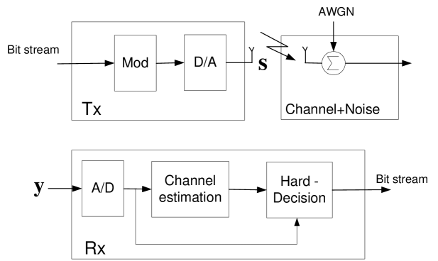
Figure 1: SISO system block diagram

The received signal $y$ is given by

$$y=hs+\rho v,$$ (1)

where $h$ is the channel response which is assumed to be known at the receiver (perfect channel knowledge), $s$ is the transmitted data (e.g QAM) and $\rho v$ is an AWGN with standard deviation $\rho$. The instantaneous antenna SNR in this case is trivial and equals to the ratio between the signal’s power to the noise’s power, meaning

$$\mbox{SNR}=\frac{|h|^{2}}{\rho^{2}}.$$ (2)

We continue with linearly decoded MIMO systems. A multiple input multiple output (MIMO) system using $M_{T}$ transmit antennas and $M_{R}$ receive antennas is illustrated in Figure 2.

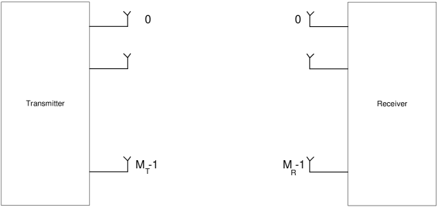
Figure 2: MIMO system block diagram (to be more detailed)

The received signal $y$ is given by

$$\mbox{\boldmath$y$}=\mbox{\boldmath$H$}_{PHY}\mbox{\boldmath$x$}+\rho\mbox{\boldmath$v$},$$ (3)

where $\mbox{\boldmath$H$}_{PHY}$ is an $\mbox{M}_{R}\times\mbox{M}_{T}$ channel matrix, $x$ is the $\mbox{M}_{T}\times 1$ transmitted vector, $v$ is a vector of i.i.d zero-mean complex Gaussian entries with unit variance and $\rho$ is the noise intensity.

In spatial multiplexing (SM) for instance, independent information streams are transmitted through the transmit antennas. Here, the transmitted vector is $\mbox{\boldmath$x$}=\displaystyle\frac{1}{\sqrt{M_{T}}}\mbox{\boldmath$s$}$, where $\mbox{\boldmath$s$}=[s_{0},s_{1},\ldots,s_{M_{T}-1}]^{T}$ is a vector of $M_{T}$ independent symbols. The factor $\displaystyle\frac{1}{\sqrt{M_{T}}}$ is introduced in order to maintain unity transmission power. The mathematical model for the received signal is

$$\mbox{\boldmath$y$}=\underbrace{\frac{1}{\sqrt{M_{T}}}\mbox{\boldmath$H$}_{PHY}}_{\mbox{\boldmath$H$}}\mbox{\boldmath$s$}+\rho\,\mbox{\boldmath$n$},$$ (4)

where $\mbox{\boldmath$H$}_{PHY}$ is the MIMO $M_{R}\times M_{T}$ channel matrix and $M_{R}\geq M_{T}$. Applying Zero-Forcing (ZF) detection gives

$$\hat{\mbox{\boldmath$s$}}=\mbox{\boldmath$H$}^{\dagger}\mbox{\boldmath$y$}=\mbox{\boldmath$s$}+\rho\mbox{\boldmath$H$}^{\dagger}\mbox{\boldmath$v$}=\mbox{\boldmath$s$}+\rho\mbox{\boldmath$Gv$},$$ (5)

where $\mbox{\boldmath$G$}=\mbox{\boldmath$H$}^{\dagger}$ is the left pseudo-inverse of $H$. The post-processing SNR of the $i-$th stream in this case reads

$$\mbox{ppSNR}_{i} = \frac{1}{\mbox{var}(\hat{s}_{i}-s_{i})}$$ (6)

$$= \frac{1}{\rho^{2}(|G_{i,0}|^{2}+\ldots+|G_{i,M_{R}-1}|^{2})}.$$

Similar results are obtained for Rx diversity and Alamouti’s space-time-coding (STC) [11]. In these schemes linear decoding is optimal so they may be viewed as a particular case of (5).

Since in general, SM is not an orthogonal transmission scheme, linear decoding is not optimal. The optimal ML decoder in this case implies exhaustive search [12]. In terms of post processing SNR, ML decoded SM differs from the linear decoding methods surveyed, in the sense that at no point in the reception process, there exists an expression for the post processing SNR. This means that another method is to be invoked.

II-B Known Approaches to SNR estimation in ML decoded SM

In this section we consider some known approaches for SNR estimation in ML decoded SM and related issues.

II-B1 SNR Estimation Based on the Capacity Formula

This approach, that was adopted by the IEEE 802.16e standard [9], uses capacity computation in order to estimate the SNR. The basic idea is to use Shannon’s expression for capacity to evaluate the SNR,

$$C = \frac{1}{M}\log_{e}\,\det\left(\mbox{\boldmath$I$}+\frac{\mbox{\boldmath$HH$}^{*}}{\rho^{2}}\right)$$

SNR Estimate $$= e^{C}-1,$$

where $M$ is the number of independent streams.

A natural question is the relevance of this metric to SNR. In order to answer this, we note that in the case of SISO, Rx diversity, and STC, this metric coincides with the standard post processing SNR. For example if we take the $1\times 2$ MRC scheme where $\mbox{\boldmath$H$}=\left[\begin{array}[]{cc}h_{0}&h_{1}\\ \end{array}\right]^{T}$ we obtain

$$C = \log\left(1+\frac{|h_{0}|^{2}+|h_{1}|^{2}}{\rho^{2}}\right),$$

which immediately implies that the estimated SNR coincides with the classical ppSNR in MRC

$$e^{C}-1=\frac{|h_{0}|^{2}+|h_{1}|^{2}}{\rho^{2}}.$$ (8)

However, despite the fact that the ability of (II-B1) to capture the SNR in the ML decoded SM case is not established, we note that (II-B1) provides a single metric, and is thus inadequate for horizontal MIMO. Horizontal transmission indicates transmitting multiple separately streams over multiple antennas such that the number of streams is more than 1 (in contrary to vertical transmission that indicates transmitting a single stream over multiple antennas).

II-B2 SNR Estimation based on Error Probability Computation

SNR and error probability are linked. Thus, an expression for the error probability may be exploited to obtain an estimate for the post processing SNR (as we will demonstrate in the next chapter). Accordingly, we consider here the closely related problem of error probability calculation in ML decoded SM.

The error probability in ML decoded SM does not have an analytic solution. One of the most prominent approaches to approximate and bound this probability is that of Paulraj and Heath [13]. They obtained the following expression for the error probability

$$\Pr\left\{\mbox{error}|\mbox{\boldmath$H$}\right\}\leq\mbox{Q}\left(\sqrt{\frac{1}{\rho^{2}}d^{2}_{\mbox{min}}(\mbox{\boldmath$H$})}\right)$$ (9)

where $d^{2}_{\mbox{min}}(\mbox{\boldmath$H$})$ is

$$d^{2}_{\mbox{min}}(\mbox{\boldmath$H$})=\mathop{\mbox{min}\|\mbox{\boldmath$H$}(\mbox{\boldmath$s$}-\mbox{\boldmath$c$})\|^{2}}_{\mbox{\boldmath$s$},\mbox{\boldmath$c$}\in\mbox{QAM}^{M_{T}},\mbox{\boldmath$s$}\neq\mbox{\boldmath$c$}}.$$ (10)

Since the computation of $d^{2}_{\mbox{min}}(\mbox{\boldmath$H$})$ requires an exhaustive search, upper and lower bounds on the minimum Euclidean distance were introduced.

$$\lambda_{\mbox{min}}^{2}(\mbox{\boldmath$H$})\frac{d_{\small{min\_QAM}}^{2}}{M_{T}}\leq d^{2}_{\mbox{min}}(\mbox{\boldmath$H$})\leq\lambda_{\mbox{max}}^{2}(\mbox{\boldmath$H$})\frac{d_{\small{min\_QAM}}^{2}}{M_{T}}$$ (11)

These bounds depend on the maximum and minimum singular values of $\mbox{\boldmath$H$}.$ In case the condition number of $H$ is high , these bounds may be loose. In addition, the computation of the singular values of $H$, especially for high ranked $H$, is a tough task by itself. Moreover, like the former approach, this method results an average estimate for the SNR over all inputs (streams), therefore it is not suitable for the per stream SNR estimation.

The rest of the paper is organized as follows. Section II includes the derivation of a series of approximations for the SNR in ML decoded SM based on a series of approximations for the per stream error probability. The chapter concludes with a low complexity implementation of the SNR estimation mechanism, based on the ML decoder itself. In Section III we present simulation results revealing the performance (in terms of SNR estimation error) of the various approximations in the horizontal and vertical cases. In the vertical case we compare our result with that of standard methods. We further show that the QPSK based methods are valid for 16QAM and 64QAM. In Section IV we summarize the results and present topics for further research.

III Proposed Method for SNR Estimation in ML Decoded SM

III-A A Series of Approximations for the Per-Stream SNR

We base our SNR estimation method on the asymptotic evaluation of the per stream error probability in ML decoded SM in high SNR. We emphasize that in order to obtain a meaningful SNR metric, the SNR estimate should satisfy (in QPSK) [14]

$$\mbox{p(error in stream i)}\approx e^{\displaystyle{-\frac{\mbox{SNR}_{i}}{2}}}.$$ (12)

We are therefore left with the problem of evaluating the per stream error probability. The conditional probability of error given the transmitted vector $s$ is (throughout we condition the probabilities on the channel matrix $H$)

$$\Pr\left\{\mbox{error}|\mbox{\boldmath$s$}\right\}=\Pr\left\{\left.\mathop{\bigcup}_{\tilde{\mbox{\boldmath$s$}}\in A(\mbox{\boldmath$s$})}\mbox{J}(\tilde{\mbox{\boldmath$s$}})<\mbox{J}(\mbox{\boldmath$s$})\right|\mbox{\boldmath$s$}\right\},$$ (13)

where $\mbox{J}(\mbox{\boldmath$s$})=\|\mbox{\boldmath$Y$}-\mbox{\boldmath$Hs$}\|^{2}$, $A(\mbox{\boldmath$s$})$ is the set of all vectors corresponding to a certain type of error, such as error in the $i-$th stream which will be represented by the set $A_{i}(\mbox{\boldmath$s$})$. Equation 13 may be bounded using the union bound

$$\Pr\left\{\mbox{error}|\mbox{\boldmath$s$}\right\} \leq \sum_{\tilde{\mbox{\boldmath$s$}}\in A(\mbox{\boldmath$s$})}{\Pr\left\{\mbox{J}(\tilde{\mbox{\boldmath$s$}})<\mbox{J}(\mbox{\boldmath$s$})|\mbox{\boldmath$s$}\right\}},$$ (14)

which may be rewritten as

$$\Pr\left\{\mbox{error}|\mbox{\boldmath$s$}\right\}\leq\sum_{\tilde{\mbox{\boldmath$s$}}\in A(\mbox{\boldmath$s$})}Q\left(\frac{\|\mbox{\boldmath$H$}(\tilde{\mbox{\boldmath$s$}}-\mbox{\boldmath$s$})\|}{\sqrt{2}\rho}\right).$$ (15)

Focusing on events of error in the $i-$th stream and averaging w.r.t $s$ gives

$$\Pr\left\{\mbox{error in i-th stream}\right\}\leq$$ (16)

$$\frac{1}{Q^{M_{T}}}\sum_{\mbox{\boldmath$s$}\in\mbox{\footnotesize{QAM}}^{M_{T}}}\sum_{\tilde{\mbox{\boldmath$s$}}\in A_{i}(\mbox{\boldmath$s$})}{\mbox{Q}\left(\frac{\|\mbox{\boldmath$H$}(\tilde{\mbox{\boldmath$s$}}-\mbox{\boldmath$s$})\|}{\sqrt{2}\rho}\right)},$$

where $Q^{-M_{T}}$ is a normalizing factor required due to the summation over all QAM points and transmit antennas. Using the upper bound on the Q-function

$$\mbox{Q}(x)\leq\frac{1}{2}\exp{\left(\displaystyle{-\frac{x^{2}}{2}}\right)},$$ (17)

we obtain a looser but simpler bound for the probability of the error

$$\Pr\left\{\mbox{error in i-th stream}\right\}\leq$$ (18)

$$\frac{1}{2}\frac{1}{Q^{M_{T}}}\sum_{\mbox{\boldmath$s$}\in\mbox{\footnotesize{QAM}}^{M_{T}}}{\sum_{\tilde{\mbox{\boldmath$s$}}\in A_{i}(\mbox{\boldmath$s$})}{e^{\displaystyle{-\frac{\|\mbox{\boldmath$H$}(\tilde{\mbox{\boldmath$s$}}-\mbox{\boldmath$s$})\|^{2}}{4\rho^{2}}}}}},$$

which may be rewritten as

$$\Pr\left\{\mbox{error in i-th stream}\right\}\leq$$ (19)

$$\frac{1}{2}\frac{1}{Q^{M_{T}}}\sum_{\mbox{\boldmath$s$}\in\mbox{\footnotesize{QAM}}^{M_{T}}}{\sum_{\mbox{\boldmath$e$}\in B_{i}(\mbox{\boldmath$s$})}{e^{\displaystyle{-\frac{\|\mbox{\boldmath$H$}\mbox{\boldmath$e$}\|^{2}}{4\rho^{2}}}}}},$$

where $\mbox{\boldmath$e$}=\tilde{\mbox{\boldmath$s$}}-\mbox{\boldmath$s$}$ and $B_{i}(\mbox{\boldmath$s$})$ is the set of vectors $e$ corresponding to $A_{i}(\mbox{\boldmath$s$})$. In order to illustrate the construction of the sets $B_{i}(\mbox{\boldmath$s$})$ we assume that the following symbol vector was transmitted

$$\mbox{\boldmath$s$}=\displaystyle\left[\begin{array}[]{c}\displaystyle\frac{-1+j}{\sqrt{2}}\\ \\ \displaystyle\frac{-1+j}{\sqrt{2}}\\ \end{array}\right],$$ (23)

as depicted in Figure 3. We focus on the probability of error in the first element, i.e., the vectors $e$ in which the first element is nonzero. All the possibilities for $e$ are illustrated in Figure 3 by the paths from the transmitted signal to any possible erroneous point.

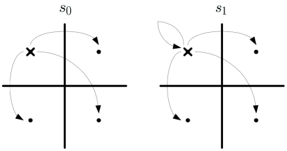
Figure 3: 2 streams constellation map

These possibilities (vectors) correspond to the following vectors $e$ in the set $B_{0}(\mbox{\boldmath$s$})$.

$$B_{0}(\mbox{\boldmath$s$}) = \sqrt{2}\left\{\left[\begin{array}[]{c}1\\ 0\\ \end{array}\right],\left[\begin{array}[]{c}1\\ 1\\ \end{array}\right],\left[\begin{array}[]{c}1\\ -1\\ \end{array}\right],\left[\begin{array}[]{c}1\\ 1-j\\ \end{array}\right],\right.$$ (50)

$$\left[\begin{array}[]{c}-j\\ 0\\ \end{array}\right],\left[\begin{array}[]{c}-j\\ 1\\ \end{array}\right],\left[\begin{array}[]{c}-j\\ -1\\ \end{array}\right],\left[\begin{array}[]{c}-j\\ 1-j\\ \end{array}\right],$$

$$\left.\left[\begin{array}[]{c}1-j\\ 0\\ \end{array}\right],\left[\begin{array}[]{c}1-j\\ 1\\ \end{array}\right],\left[\begin{array}[]{c}1-j\\ -1\\ \end{array}\right],\left[\begin{array}[]{c}1-j\\ 1-j\\ \end{array}\right]\right\}.$$

Next, we further simplify the expression, by canceling the dependence of the sets $B_{i}(\mbox{\boldmath$s$})$ on the transmitted vector $s$ and turn to unified sets $B_{i}$

$$B_{i}=\bigcup_{\mbox{\boldmath$s$}}B_{i}(\mbox{\boldmath$s$}).$$ (51)

Using the unified sets, the error probability is approximated by

$$\Pr\left\{\mbox{error in i-th stream}\right\}\approx{\sum_{\mbox{\boldmath$e$}\in B_{i}}{e^{\displaystyle{-\frac{\|\mbox{\boldmath$H$}\mbox{\boldmath$e$}\|^{2}}{4\rho^{2}}}}}}.$$ (52)

Note that the approximation in (52) is based on the fact that elements in the sets $B_{i}$ are unique, so the summation in (52) is different than that in (19). Focusing on the high SNR regime, (52) may be well approximated by the max-log approximation as

$$\Pr\left\{\mbox{error in i-th stream}\right\}\approx{e^{\displaystyle{-\mathop{\mbox{min}}\limits_{\mbox{\boldmath$e$}\in B_{i}}\frac{\|\mbox{\boldmath$H$}\mbox{\boldmath$e$}\|^{2}}{4\rho^{2}}}}}.$$ (53)

This means that the sets $B_{i}$ may be replaced with abbreviated sets $\hat{B}_{i}$ that omit elements that lead identical value of $\|\mbox{\boldmath$H$}\mbox{\boldmath$e$}\|^{2}$, such that

$$\Pr\left\{\mbox{error in i-th stream}\right\} \approx {e^{\displaystyle{-\mathop{\mbox{min}}\limits_{\mbox{\boldmath$e$}\in B_{i}}\frac{\|\mbox{\boldmath$H$}\mbox{\boldmath$e$}\|^{2}}{4\rho^{2}}}}}$$ (54)

$$= {e^{\displaystyle{-\mathop{\mbox{min}}\limits_{\mbox{\boldmath$e$}\in\hat{B}_{i}}\frac{\|\mbox{\boldmath$H$}\mbox{\boldmath$e$}\|^{2}}{4\rho^{2}}}}}.$$

For instance, the vectors $\left[\begin{array}[]{cc}\sqrt{2}&0\\ \end{array}\right]^{T}$ and $\left[\begin{array}[]{cc}-j\sqrt{2}&0\\ \end{array}\right]^{T}$ lead to the same cost, so one of them may be omitted. Moreover, noting that some pairs $\mbox{\boldmath$a$},\mbox{\boldmath$b$}$ of elements in $B_{i}$

$$\mbox{\boldmath$b$}=\alpha\mbox{\boldmath$a$},|\alpha|>1$$ (55)

leads to the understanding that the cost of $b$ is $\alpha^{2}$ the cost of $a$, so $b$ may also be omitted from the abbreviated set $\hat{B}_{i}$. An example to such a pair is

$$\displaystyle\left[\begin{array}[]{c}\sqrt{2}\\ \\ \sqrt{2}\\ \end{array}\right],$$ (59)

and

$$\displaystyle\left[\begin{array}[]{c}\sqrt{2}+j\sqrt{2}\\ \\ \sqrt{2}+j\sqrt{2}\\ \end{array}\right].$$ (63)

These arguments lead to the abbreviated set $\hat{B}_{0}$

$$\hat{B}_{0}=\sqrt{2}\left\{\left[\begin{array}[]{c}1\\ 0\\ \end{array}\right],\left[\begin{array}[]{c}1\\ 1\\ \end{array}\right],\left[\begin{array}[]{c}1\\ j\\ \end{array}\right],\left[\begin{array}[]{c}1\\ -1\\ \end{array}\right],\left[\begin{array}[]{c}1\\ -j\\ \end{array}\right],\right.$$ (74)

$$\left[\begin{array}[]{c}1\\ 1-j\\ \end{array}\right],\left[\begin{array}[]{c}1\\ 1+j\\ \end{array}\right],\left[\begin{array}[]{c}1\\ -1+j\\ \end{array}\right],\left[\begin{array}[]{c}1\\ -1-j\\ \end{array}\right],$$ (83)

$$\left.\left[\begin{array}[]{c}1+j\\ 1\\ \end{array}\right],\left[\begin{array}[]{c}1+j\\ -1\\ \end{array}\right],\left[\begin{array}[]{c}1+j\\ j\\ \end{array}\right],\left[\begin{array}[]{c}1+j\\ -j\\ \end{array}\right]\right\}.$$ (92)

An interesting outcome resulting from the abbreviation procedure is that the sets $\hat{B}_{i},\,\hat{B}_{j},\,i\neq j$ differ only in a single vector, denoted here as the first. The first vector $\mbox{\boldmath$b$}_{i}$ in the $i-$th set, refers to the error vector in which only the $i-$th element is nonzero. This implies that the sets $\hat{B}_{i}$ may be written as

$$\hat{B}_{i}=\{\mbox{\boldmath$b$}_{i},C\},$$ (93)

where the set $C$ is the intersection of all sets $\hat{B}_{i}$,

$$C=\bigcap^{i}\hat{B}_{i}.$$ (94)

III-B Low Complexity Implementation

The structure of (54) implies that the SNR may be evaluated using the ML decoder. Such a decoder is depicted in Fig. 4.

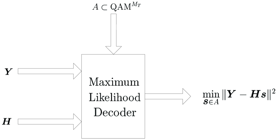
Figure 4: Maximum likelihood decoder

The ML decoder uses the inputs $Y$ and $H$ and performs a search over all vectors from a predefined set $\mathcal{A}$ (usually $\mathcal{A}\subset\mbox{QAM}^{M_{T}}$). The output of the decoder is $\mathop{\mbox{min}}\limits_{\mbox{\boldmath$s$}\in A_{ml}}\|\mbox{\boldmath$Y$}-\mbox{\boldmath$Hs$}\|^{2}$. We notice that with setting $\mbox{\boldmath$Y$}=0$ and searching over $\hat{B}_{i}$ instead of $\mathcal{A}$ we can evaluate the SNR introduced in (54). Since the sets $\hat{B}_{i}$ are significantly smaller that $\mathcal{A}$ and since the SNR calculation process is done once for many information bits, the SNR estimation task embodies a small to negligible fraction of the ML decoder resources.

To set ideas straight, we assume we have a 10 symbol QPSK allocation of 2 antenna SM. The data decoding process invokes the ML decoder twice for each transmitted bit. Each search is over $\frac{1}{2}\mbox{QPSK}^{2}$ or 8 constellation points. All in all we have 80 searches over 8 constellation points. In this allocation a single SNR calculation is needed, so we have the ML decoder invoked twice (once for each stream) to search a set of 9 elements. This means that in this case the extra overhead introduced by the SNR calculation is $\displaystyle\frac{2}{80}=2.5\%$.

We note that in many receivers the optimal ML decoder considered here is replaced with lower complexity near optimal decoders ([15],[16]). In this case, the SNR estimation methods may be modify to accommodate near optimal ML decoders.

IV Simulation Results

In this chapter we present simulation studies investigating the performance of the series of error probability approximations presented in the previous chapter and the corresponding estimated SNR. The simulation results reveal the following interesting virtues of the proposed SNR estimation methods.

• The performance of the proposed methods are consistent with the level of approximation. This means that the most accurate approximation (16) relying on solely on the union bound is superior to all other, while the simplest (54) is inferior to all others.

• The approximations introduce small performance degradation, so the performance of all methods is similar.

• In case of vertical encoding (where other methods are applicable) the proposed methods slightly outperform the existing method. This serves as a good ”sanity check” for the methods.

• SNR should not depend on the modulation employed. Thus, we examine the application of a QPSK based SNR estimation mechanism also for higher modulations. We show that the QPSK based mechanism gives plausible results also for 16QAM.

IV-A The Simulation Setup

In order to investigate the performance of the proposed methods, we used the following procedure.

1. Randomly generate 2000 i.i.d Rayleigh distributed $2\times 2$ matrices $H$.

   1. Using each matrix transmit $10^{6}$ vectors $\mbox{\boldmath$s$}\in\mbox{QAM}^{2}$, and decode the vectors $s$ from

      $$\mbox{\boldmath$y$}=\frac{1}{\sqrt{2}}\mbox{\boldmath$Hs$}+\rho\,\mbox{\boldmath$n$},$$ (95)

      using the ML decoder.

   2. Compute the empiric SER in each stream.

   3. Compute the empiric post processing SNR implied by the per stream SER according to

      $$\mbox{SNR}_{i}=-2\log\mbox{SER}_{i}.$$ (96)

   4. Compute the estimated SNR for QPSK at each stream according to the three approximations (16), (52) and (54) (denoted as ”Union Bound”, ”Full-sum approx” and ”Max-log approx” respectively in the graphs).

   5. Compute the empiric joint SER for both streams.

   6. Compute the empiric post processing SNR implied by the joint SER.

   7. Compute the joint estimated SNR for both streams based on the per stream estimated SNR through the equation

      $$\hat{\mbox{SNR}}_{vert}[\mbox{dB}]=\frac{1}{2}\left(\hat{\mbox{SNR}}_{1}[\mbox{dB}]+\hat{\mbox{SNR}}_{2}[\mbox{dB}]\right),$$ (97)

      where $\hat{\mbox{SNR}}_{i}$ is the estimated SNR in the $i-$th stream based on (16), (52) and (54).

   8. Compute the capacity based joint SNR, $\hat{\mbox{SNR}}_{cap}$, according to the capacity method (II-B1) (denoted as ”Capacity” in the graphs).

IV-B Results for Horizontal QPSK

The simulation results show that the standard deviation of the error is approximately 2-3dB for each stream using both the full-sum and max-log approximations. Moreover, the standard deviation of the error when using the union bound approximation is some 1dB, which means only 1dB better than the former approximations. These differences are well shown in Figure 5. We note that each graph was compensated with its mean error so it is symmetric around zero. It is easy to see that the max-log approximation based SNR and the full-sum approximation based SNR are very similar for stream 0. (The same holds for stream 1, too). Hence we may conclude that the max-log approximation introduces negligible performance degradation.

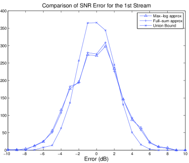
Figure 5: Distribution of the SNR estimation error respective to stream 0.

IV-B1 Vertical QPSK

In order to expand the algorithm to support a single SNR we defined the SNR to be the logarithmic average of the 2 per stream SNRs

$$\mbox{SNR}_{Vertical}=\frac{1}{2}(\mbox{SNR}_{0}+\mbox{SNR}_{1}),$$ (98)

for the union bound, full-sum and max-log approximations. Fig. 6 shows the error distribution of the vertical SNR calculation along with the capacity-based SNR as described in (II-B1). The graph shows that there is a slight advantage for the new algorithm (for both the full-sum and max-log approximations, which similarly to the horizontal case have very close performance) over the capacity based SNR in terms of error standard deviation. As expected, the union bound SNR is superior to all three other calculations, having a standard deviation of approximately 1dB.

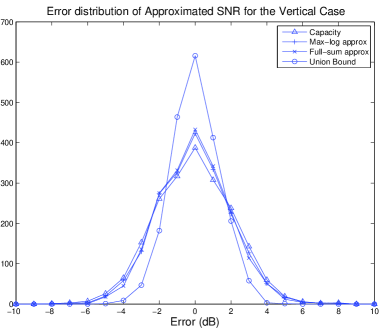
Figure 6: Distribution of the SNR estimation error for the vertical case

IV-C 16QAM and 64QAM

As mentioned, the SNR should not be constellation dependent. Therefore we examine the new method when 16QAM and 64QAM constellations are applied. The only modification needed is the calculation of the reference SNR which for QPSK was introduced in (12). In the case of 16QAM the error probability is given by

$$\mbox{p(error in stream i)}=e^{\displaystyle{-\frac{\mbox{SNR}_{i}}{10}}},$$ (99)

and in the case of 64QAM it reads

$$\mbox{p(error in stream i)}=e^{\displaystyle{-\frac{\mbox{SNR}_{i}}{42}}},$$ (100)

The values in the exponent denominators are obtained from the normalized constellation construction as depicted in the IEEE 802.16 standard [9].

IV-C1 Preliminary verification

A straight forward extension of the ideas demonstrated in Section III-A is to develop a 16QAM based SNR estimation mechanism for 16QAM transmission and a 64QAM mechanism for 64QAM transmission. The performance of a 16QAM based mechanism for 16QAM transmission is given in Fig. 7. Simulation results show that the performance in the 16QAM case is similar to that in QPSK (the standard deviation is approximately 2dB) .

Bearing in mind that SNR should be a modulation independent measure, we suggest to employ a QPSK based SNR estimation mechanism for other modulations as 16QAM and 64QAM. Obviously, this approach leads to a more efficient mechanism since it implies a single mechanism for all modulations and more important, it makes use of the smaller search spaces respective to QPSK (the 16QAM based set, which is not introduced in this work, consists of 50 entries compared to only 13 entries in the QPSK based set, as given in (74). The performance of a QPSK based mechanism for 16QAM transmission is given in Fig. 7. Note that the performance of the QPSK based mechanism is slightly inferior to the 16QAM based mechanism, however, this degradations seems negligible.

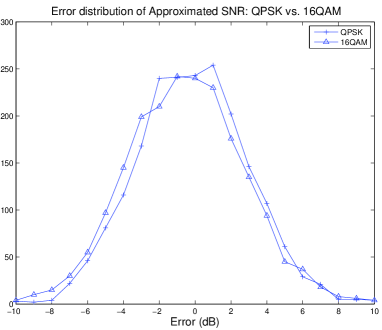
Figure 7: Distribution of the SNR estimation for QPSK and 16QAM

IV-C2 Per Stream SNR for 16QAM

Simulation report indicated a standard deviation of  2.2dB for the union bound SNR calculation and  3dB for the approximated SNR calculation For the horizontal case. As for the vertical case, similarly to QPSK, a small degradation in means of error standard deviation ($\sim 0.1$dB) was achieved using the approximated SNR over the traditional capacity based SNR. Figure 8 shows the distributions of the SNR error for stream 0.

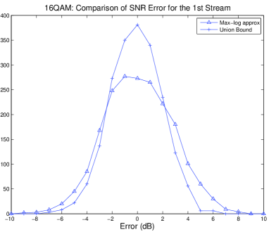
Figure 8: Distribution of the SNR estimation error of stream 0 for 16QAM

V Discussion and Conclusions

In this paper, we develop methods for estimating the post processing SNR in ML decoded SM. Our results include a series of SNR estimation methods based on various approximations for the per stream error probability in ML decoded SM. We propose a very low complexity implementation of the SNR estimation method, based on the ML decoder itself with negligible overhead over the routine employment of the decoder for data detection. We show that QPSK based algorithm provides plausible performance also for the higher modulations, so that a single SNR estimation mechanism is required for link adaptation. Per stream SNR estimation for ML decoded SM may play an important role in UL and DL SDMA schemes where each stream corresponds to a different user, hence per stream SNR estimation is required [17], [18], [19]

References

- [1] G. Holland, N. Vaidya, and P. Bahl, “A rate-adaptive MAC protocol for multi-hop wireless networks,” in Proc. ACM MobiCom ’01,, pp. 236–251, July 2001.
- [2] O. Queseth, G. Gessler, and M. Frodigh, “Algorithms for link adaptation in GRPS,” in Proc. IEEE VTC 99, pp. 943–947, May 1999.
- [3] J. Khun-Jush, P. Schramm, U. Wachsmann, and W. Wenger, “Algorithms for link adaptation in GRPS,” in Proc. IEEE VTC 99, pp. 2667–2671, May 1999.
- [4] Z. Lin, G. Malmgren, and J. Torsner, “System performance analysis of link adaptation in HiperLAN Type 2,” in Proc. IEEE VTC 00 Fall,, vol. 4, pp. 1719–1725, May 2000.
- [5] J. Habetha, and D. Calvo de No, “New adaptive modulation and power control algorithms for HIPERLAN/2 multihop ad hoc networks,” in Proc. European Wireless,, September 2000.
- [6] K. Balachandran, S. R. Kadaba, and N. Sanjiv, “Channel quality estimation and rate adaptation for cellular mobile radio,” IEEE Journal on Selected Areas in Communications, pp. 1244–1256, July 1999.
- [7] P. W. C. Chan, and R. S. Cheng, “Optimal power allocation in zero-forcing MIMO-OFDM downlink with multiuser diversity,” The 14th IST Mobile and Wireless Communications Summit, November 2005.
- [8] Z. Chen, R. Chen, J. G. Andrews, R. W. Heath Jr., and B. L. Evans, “Low complexity user selection algorithms for multiuser MIMO systems with block diagonalization,” Conference Record of the Thirty-Ninth Asilomar Conference on Signals, Systems and Computers, pp. 628–632, November 2005.
- [9] IEEE 802.16 Working Group, IEEE 802 Part 16: Air interface for croadband wireless access systems, December 2007.
- [10] D. Yao, A. Camargo, and A. Czylwik, “Adaptive MIMO transmission scheme for BICM-OFDM wireless systems,” COST 2100 TD(08)509, June 2008.
- [11] S. M. Alamouti, “A simple transmit diversity technique for wireless communications,” IEEE Journal on Selected Areas in Communications,, vol. 16, no. 8, pp. 1451–1458, October 1998.
- [12] A. Paulraj, R. Nabar, and D. Gore, Introduction to Space-Time Wireless Communications. Cambridge, 2003.
- [13] R. W. Heath Jr., and A. Paulraj, “Switching between diversity and multiplexing in MIMO systems,” IEEE Transactions on Communications,, vol. 53, no. 6, pp. 962–968, June 2005.
- [14] A. Goldsmith, Wireless Communications. Cambridge University Press, 2005.
- [15] W. U. Chung, and P. M. Hsi, “A low complexity scalable MIMO detector,” International Conference On Communications And Mobile Computing, pp. 605–610, 2006.
- [16] V. Paminer, Y. Delignon, W. Sawaya, and D. Boulingiirzi, “A low complexity suboptimal MIMO receiver: The combined ZF-MLD algorithm,” The 14th IEEE 2003 International Symposium on Persona1,lndoor and Mobile Radio Communication Proceedings, pp. 2271–2275, 2003.
- [17] Y. Taesang, and A. Goldsmith, “Optimality of zero-forcing beamforming with multiuser diversity,” IEEE International Conference on Communications, vol. 1, pp. 542–546, May 2005.
- [18] Q. H. Spencer, A. L. Swindlehurst, and M. Haardt, “Zero-forcing methods for downlink spatial multiplexing in multiuser MIMO channels,” IEEE Transactions on Signal Processing, vol. 52, no. 2, pp. 461–471, February 2004.
- [19] Y. Taesang, and A. Goldsmith, “On the optimality of multiantenna broadcast scheduling using zero-forcing beamforming,” IEEE Journal on Selected Areas in Communications, vol. 24, pp. 528–541, March 2006.