The host galaxy of a narrow-line Seyfert 1 galaxy RE J1034+396 with X-ray quasi-periodic oscillations

Abstract

Using simple stellar population synthesis, we model the bulge stellar contribution in the optical spectrum of a narrow-line Seyfert 1 galaxy RE J1034+396. We find that its bulge stellar velocity dispersion is $67.7\pm 8$ km s${}^{-1}$ . The supermassive black hole (SMBH) mass is about $(1-4)\times 10^{6}M_{\odot}$ if it follows the well-known $M_{\rm BH}-\sigma_{*}$ relation found in quiescent galaxies. We also derive the SMBH mass from the H$\beta$ second moment, which is consistent with that from its bulge stellar velocity dispersion. The SMBH mass of $(1-4)\times 10^{6}M_{\odot}$ implies that the X-ray quasi-periodic oscillation (QPO) of RE J1034+396 can be scaled to a high-frequency QPO at 27-108 Hz found in Galactic black hole binaries with a 10 $M_{\odot}$ black hole. With the mass distribution in different age stellar populations, we find that the mean specific star formation rate (SSFR) over past 0.1 Gyr is $0.0163\pm 0.0011$ $\rm Gyr^{-1}$, the stellar mass in the logarithm is $10.155\pm 0.06$ in units of solar mass, and the current star formation rate is $0.23\pm 0.016~{}M_{\odot}~{}\rm yr^{-1}$. RE J1034+396 does not follow the relation between the Eddington ratio and the SSFR suggested by Chen et al., although a larger scatter in their relation. We also suggest that about 7.0% of the total H$\alpha$ luminosity and 50% of the total [O ii] luminosity come from the star formation process.

1 INTRODUCTION

It is thought that active galactic nuclei (AGN) are scaled-up versions of Galactic black hole binaries (BHBs; Gierlinski et al. 2008 and reference therein). The power spectrum of the X-ray variability in BHBs shows the quasi-periodic oscillations of 0.01-450 Hz(QPOs; Rimillard & McClintock 2006). It is believed that we can also find the QPOs in AGN, on the similar behavior of accretion flow around the black hole (BH). Comparing to a BH of 10 $M_{\odot}$ in BHBs, the typical high-frequency QPOs of 100 Hz would be smaller by $10^{6}$ (i.e., $\sim 10^{-4}$ Hz) for a supermassive black hole ($M_{\rm BH}$ ; SMBH) of $10^{7}M_{\odot}$ if the QPO frequencies scale inversely with the BH mass (Rimillard & McClintock 2006).

With a long XMM-Newton observation (91 ks), Gierlinski et al. (2008) detected a significant QPO signal ($\nu=2.7\times 10^{-4}\rm Hz$, corresponding to a period of about 1 hour) for a nearby (z=0.043) spiral active galaxy RE J1034+396 (J2000, RA=158.66082, DEC=39.64119). It is optically classified as a narrow-line Seyfert 1 galaxy (NLS1), with similar small line width for the high-ionization and low-ionization emission lines (Puchnarewicz et al. 1998), and a very soft X-ray spectrum (Grupe et al. 2004; Casebeer et al. 2006). NLS1s are thought to be a special subclass of AGN harboring relatively small but growing SMBHs, compared with other broad-line Seyfert 1 galaxies (BLS1s; e.g. Osterbrock & Pogge 1985; Boller, Brandt & Fink 1996; Mathur 2000). By methods of the standard accretion disk model fitting of spectral energy distribution (SED; Puchnarewicz et al. 2001), the slim disk fitting of SED (Wang et al., 1999; Wang & Netzer 2003), the full width at half-maximum (FWHM) of the H$\beta$ line, [O iii] FWHM, and soft X-ray luminosity, the SMBH mass in RE J1034+396 can not be determined very well, from $6.3\times 10^{5}$ to $3.6\times 10^{7}M_{\odot}$ (Bian et al. 2004; Wang & Lu 2001). Its QPO type (high-frequency or low-frequency QPOs) can not be uniquely identified (Gierlinski et al. 2008).

In the past two decades, there has been striking progress in finding more reliable methods to calculate SMBHs masses in AGN through the line width, $\Delta V$, of H$\beta$ (or H$\alpha$, Mg ii , C iv ) from the broad line region (BLR) and the BLR size, $R_{\rm BLR}$ (e.g., Kaspi et al. 2000; McLure & Dunlop 2004; Bian & Zhao 2004; Peterson et al. 2004; Greene & Ho 2005b; Bian et al. 2008). There are mainly two ways to parameterize the line widths of broad emission lines, i.e., FWHM and the second moment ($\sigma_{line}$) (e.g. Bian et al. 2008). The second moment of the broad components of the H$\beta$ line provides a more precise measurement of the SMBH mass because the H$\beta$ profile is non-Gaussian in NLS1s. It is suggested that the mean value of the SMBH masses in NLS1s from the H$\beta$ second moment is larger by about 0.50 dex than that from FWHM (Bian et al. 2008). The well-known $M_{\rm BH}-\sigma_{*}$ relation of inactive galaxies (Tremaine et al. 2002) can also be used to estimate the SMBH mass when the stellar velocity dispersion, $\sigma_{*}$, is available (Kauffmann et al. 2003; Onken et al. 2004; Greene & Ho 2006).

The X-ray QPOs frequency may depend on the mass and the spin of BH (Rimillard & McClintock 2006). The SMBH masses are important in the study of QPOs in AGN. Here we use the the Sloan Digital Sky Survey (SDSS; Abazajian et al. 2009) data of this object to determine its SMBH mass by its $\sigma_{*}$ and H$\beta$ second moment instead of H$\beta$ FWHM in Bian et al. (2004), as well as the star formation history of its host bulge by the simple stellar population (SSP) synthesis. All of the cosmological calculations in this paper assume $H_{0}=70\rm{~{}km~{}s^{-1}~{}Mpc^{-1}}$, $\Omega_{M}=0.3$, and $\Omega_{\Lambda}=0.7$.

2 Data and Analysis

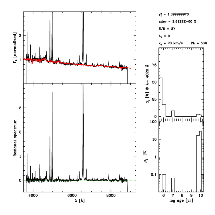
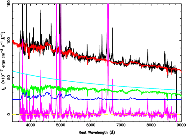
Figure 1: Results of simple stellar population (SSP) synthesis for the SDSS spectrum of RE J1034+396. Top panel: the left panels are the observed and the synthesis spectra (black and red, respectively) , and the residual spectrum. The panels on the right show the the flux-fraction $x_{j}$ and mass-fraction $\mu_{j}$ versus the ages of the simple stellar populations. Bottom panel: the black line is the observed SDSS spectrum corrected for Galactic extinction in the rest frame. The cyan line is the power-law continuum. The green line is the host contribution. The blue line is the Fe ii spectrum. The magenta line is the residue. The red line is the composition of the host contribution, Fe ii lines and the power-law continuum.

The SDSS used a dedicated 2.5-m wide-field telescope at Apache Point Observatory near Sacramento Peak in Southern New Mexico to conduct an imaging and spectroscopic survey for about 1/4 sky area. The SDSS data have been made public in a series of yearly data releases and the present is the Seventh Data Release (DR7), including data up to the end of SDSS-II in July, 2008.

The optical spectrum of RE J1034+396 is downloaded from SDSS DR7. Its spectrum covers the wavelength range of 3800-9200 Å with a spectral resolution of $1800<R<2100$. At its redshift of 0.043, the projected fiber aperture diameter of 3” is about 2.4 kpc, containing most light from its bulge. With nuclei spectrum superimposed on it, the stellar absorption features in its SDSS spectrum provide us the possibility to investigate the property of its host bulge, including the bulge stellar velocity dispersion, the stellar mass, and the star formation history. We did not apply aperture correction to the stellar velocity dispersion because this effect can be omitted for $z<0.3$ (Bernardi et al. 2003).

We outline our steps to do the SDSS spectral analysis. (1) We use SSP synthesis (STARLIGHT; Cid Fernandes et al. 2005) to model the stellar contribution in the Galactic extinction-corrected spectrum in the rest frame (Cid Fernandes et al. 2005; Bian et al. 2006, 2007, 2008). The Galactic extinction law of Cardelli, Clayton & Mathis (1989) with $R_{V}=3.1$ is adopted, which is also used for the host extinction with V-band extinction (from 0 mag to 5.0 mag). We use 45 default templates in Cid Fernandes et al. (2005), which are calculated from the model of Bruzual & Charlot (2003). The linear combination of 45 templates is used to represent the host bulge spectrum. These 45 templates comprise 15 ages, $t=$ 0.001, 0.00316, 0.00501, 0.01, 0.02512, 0.04, 0.10152, 0.28612, 0.64054, 0.90479, 1.434, 2.5, 5, 11 and 13 Gyr, and three metallicities, $Z=$ 0.2, 1 and 2.5 $Z_{\odot}$ (Cid Fernandes et al. 2005). At the same time as the SSP fit, we add a power-law component in the code to represent the AGN continuum emission, and an optical Fe ii template from the prototype NLS1 I ZW 1 (Boroson & Green 1992) to model the Fe ii emission. We exclude the AGN mission lines, such as H Balmer lines, [O ii] $\lambda$3727, [Ne iii] $\lambda$3869, [O iii] $\lambda\lambda$4959, 5007, [N ii] $\lambda\lambda$6548, 6583, [S ii] $\lambda\lambda$6717, 6731.

The synthetic spectrum is built using the following equation,

$$M_{\lambda}=M_{\lambda_{0}}\left[\sum_{j=1}^{N_{*}}x_{\rm j}b_{\rm j,\lambda}r_{\lambda}\otimes G(v_{0},v_{d})+x_{\rm fe}\otimes G(v_{\rm fe},\sigma_{\rm fe})\right]$$ (1)

where $b_{\rm j,\lambda}$ is the $j^{\rm th}$ template normalized at $\lambda_{0}=4020$ Å, $x_{j}$ is the flux fraction at 4020 Å, $M_{\lambda_{0}}$ is the synthetic flux 4020 Å, $r_{\lambda}\equiv 10^{-0.4(A_{\lambda}-A_{\lambda 0})}$ is the reddening term by V-band extinction $A_{V}$, and $G(v_{0},v_{d})$ is the line-of-sight stellar velocity distribution, modeled as a Gaussian centered at velocity $v_{0}$ and broadened by the velocity dispersion $v_{d}$. Due to different velocity dispersion in the stellar lines and Fe ii lines, we use another line-of-sight Fe ii velocity distribution $G(v_{\rm fe},\sigma_{\rm fe})$ for the Fe ii emission. $x_{\rm fe}$ is the Fe ii flux-fraction at 4020Å. The line-of-sight Fe ii velocity distribution $G(v_{\rm fe},\sigma_{\rm fe})$ is also modeled as a Gaussian centered at velocity $v_{\rm fe}$ and broadened by the velocity dispersion $\sigma_{\rm fe}$. We first fit the Fe ii lines and the continuum in the fitting windows. And we find that $\sigma_{\rm fe}=411\pm 46{\rm km\ s}^{-1}$. $\sigma_{\rm fe}$ is fixed by 411 km/s in the fitting of SSP and Fe ii . When we change $\sigma_{\rm fe}$, the SSP and Fe ii fitting results do not change, considering the errors. We also exclude the Fe ii emissions and do the SSP fit, considering the errors, the SSP results do not change. The best fit is reached by minimizing reduced $\chi^{2}$,

$$\chi^{2}(x,M_{\lambda_{0}},A_{\rm V},v_{0},v_{d})=\sum_{\lambda=1}^{N_{\lambda}}\left[\left(O_{\lambda}-M_{\lambda}\right)w_{\lambda}\right]^{2}/N$$ (2)

where the weighted spectrum $w_{\lambda}$ is defined as the noise associated with each spectral bin as reported by the SDSS pipeline output, N is the total unmasked pixels. $\chi^{2}$ is calculated by the difference between observed spectrum and the model spectrum in the fitting of SSP and Fe ii . For RE J1034+396, the best fit of SSP and Fe ii gives $\chi^{2}=1.4$ (Fig 1). We find that $A_{V}=0$, and the host extinction can be neglected (Fig 1). Through above spectral synthesis, we can obtain some parameters, such as bulge velocity dispersion $v_{d}$, flux-fraction $x_{j}$, mass-fraction $\mu_{j}$, stellar mass $M_{*}$. The mass-flux ratio can be found in STARLIGHT manual on the web site http://www.starlight.ufsc.br/. The results are shown in Fig. 1 and Table 1.

With the simulation, it is suggested that the uncertainty of SSP results can be given by the effective starlight signal-to-noise (S/N) at 4020 Å (Cid Fernandes et al. 2005; Bian et al. 2007). The S/N at 4020 Å is 37 and the starlight fraction at 4020 Å is about 43% (Table 1). Therefore the effective starlight S/N at 4020 Å is about 16, corresponding to an uncertainty of 8 km s${}^{-1}$ for the velocity dispersion, 7% for the mass-fraction, 8% for the flux-fraction, 0.06 dex for stellar mass $logM_{*}$ (Cid Fernandes et al. 2005; Bian et al. 2007). We adopt 10% as the uncertainty of host bulge flux fraction.

(2) Considering the broad wing in the H$\beta$ line profile, two broad components are used to model broad H$\beta$ profile from BLRs. The H$\beta$ line from the narrow line regions (NLRs) has the same profile as the [O iii] line from NLRs. Two components are used to model the asymmetric [O iii] line profile, and two components are used to model H$\beta$ line profile from NLRs (Bian et al. 2008). Therefore, total four Gaussians are used to model the H$\beta$ line profile, and two sets of two Gaussians are used to model the [O iii] $\lambda\lambda 4959,5007$ lines. As the same as the H$\beta$ profile, four Gaussians are used to model the H$\alpha$ profile (two broad components from BLRs and two narrow components from NLRs), and two sets of two Gaussian are used to model the [N ii] $\lambda\lambda 6548,6583$ lines. We take the same line width for each corresponding component of [O iii] $\lambda\lambda 4959,5007$ and H$\beta$ from NLRs, fix the flux ratio of [O iii] $\lambda 4959$ to [O iii] $\lambda 5007$ to be 1:3, and set the wavelength separation to the laboratory value. We take the same line width for each corresponding component of [N ii] $\lambda\lambda 6548,6583$ and H$\alpha$ from BLRs, fix the flux ratio of [N ii] $\lambda 6548$ to [N ii] $\lambda 6583$ to be 1:3, and set the wavelength separation to the laboratory value. For RE J1034+396, the best fits of the H$\beta$ , H$\alpha$ lines give reduced $\chi^{2}=2.2,\chi^{2}=2.14$, respectively. The results are shown in Fig. 2 and Table 2. The third component of the H$\beta$ line from NLRs is weaker, the results do not change if we remove this weaker component.

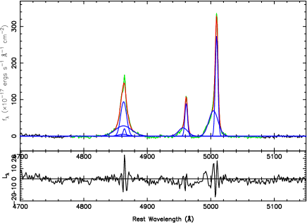
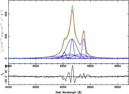
Figure 2: An example of the line fit for RE J1034+396. Top panel: the line fit for H$\beta$ and [O iii] line. The black line is the original spectrum after Galactic-extinction correction, the starlight subtraction, the power-law continuum and the Fe ii subtraction in the rest frame. The residual is shown at the bottom. The multiple Gaussian components are in blue and the sum of them is in red. The fitting window is in green. Bottom panel: the line fit for H$\alpha$ and [N ii] line. The line colors are the same to that in top panel.

3 Result and Discussion

Table 1: The host bulge properties of RE J1034+396

$\sigma_{*}({\rm km\ s}^{-1})$	$logM_{*}(M_{\odot})$	$SSFR(\rm Gyr^{-1})$	$f_{\rm host}$
(1)	(2)	(3)	(4)
$67.7\pm 8$	$10.155\pm 0.06$	$0.0163\pm 0.0011$	$43\pm 4$%

Note. Col(1): the host bulge stellar velocity dispersion; Col(2): the stellar mass; Col(3): the host bulge specific star formation rate; Col(4): the host bulge flux fraction at 4020 $\AA$ with 10% uncertainty.

Table 2: The emission lines properties of RE J1034+396

	FWHM${}^{a}$	flux${}^{b}$
H$\beta$	$1690\pm 296$	$1.1\pm 0.84$
	$617\pm 155$	$0.88\pm 0.73$
	$1022\pm 4592^{n}$	$0.10\pm 0.63$
	$292\pm 114^{n}$	$0.12\pm 0.13$
[O iii]	$1023\pm 18^{n}$	$1.26\pm 0.03$
	$292\pm 5^{n}$	$1.43\pm 0.03$
H$\alpha$	$969\pm 552$	$3.98\pm 3.15$
	$3804\pm 1100$	$2.25\pm 0.39$
	$272\pm 25^{n}$	$1.16\pm 0.25$
	$1162\pm 275^{n}$	$1.09\pm 2.75$
[N ii] $\lambda 6583$	$278\pm 80^{n}$	$1.16\pm 0.08$
	$1162\pm 287^{n}$	$1.1\pm 2.81$
Fe ii	$967\pm 108$	$1.76\pm 0.2^{c}$

Note. ${}^{a}$: FWHM of a Gaussian profile in units of km s${}^{-1}$ . ${}^{b}$: in units of $10^{-14}~{}\rm erg~{}s^{-1}~{}cm^{-2}$. ${}^{c}$: Fe ii flux between 4434 Å and 4684 Å. ${}^{n}$: the components from NLRs. The second weaker broad component of H$\alpha$ is probably due to the contribution from the continuum subtraction.