Effect of Phase Factor in the Geometric Entanglement Measure of Three-Qubit States
Sayatnova Tamaryan
Theory Department, Yerevan Physics Institute, Yerevan-36, 375036, Armenia
Hungsoo Kim
The Institute of Basic Science, Kyungnam University, Masan, 631-701, Korea
Mu-Seong Kim, Kap Soo Jang, DaeKil Park
Department of Physics, Kyungnam University, Masan, 631-701, Korea
Abstract
Any pure three-qubit state is uniquely characterized by one phase and four positive
parameters. The geometric measure of entanglement as a function of state parameters
can have different expressions. Each of expressions has its own applicable domain
and thus the whole state parameter space is divided into subspaces that are ranges
of definition for corresponding expressions. The purpose of this paper is to examine
the applicable domains for the most general qubit-interchange symmetric three-qubit
states. First, we compute the eigenvalues of the non-linear eigenvalue equations
and the nearest separable states for the permutation invariant
three-qubit states with a fixed phase. Next, we compute the geometric entanglement
measure, deduce the boundaries of all subspaces,
and find allocations of highly and slightly entangled states. It is shown that
there are three applicable domains when the phase factor is while other
cases have only two domains. The emergence of the three domains is due to the
appearance of the additional W-state. We show that most
of highly entangled states reside near the boundaries of the domains and states
located far from the boundaries become less-entangled and eventually go to the
product states. The neighbors of W-state are generally more entangled than the
neighbors of Greenberger-Horne-Zeilinger(GHZ) state from the aspect of the geometric
measure. However, the range of the GHZ-neighbors is much more wider than the range
of the W-neighbors.
I Introduction
Entanglement is a property of quantum states that does not exist classically.
Two or more subsystems of a quantum system are said to be entangled if the state of the
entire system cannot be described in terms of a state for each of the
subsystems wern-89 . This property of composite quantum systems, which exhibits
quantum correlations between subsystems, is a resource for many processes in quantum
information theory ek-91 ; ben-wies ; ben-per ; ital-09 .
Since the profound measures of entanglement, i.e. the entanglement of formation and
distillation ben-schum ; ben-vinc ; woot-98 ; vid-cir , have not been properly
generalized to multiparticle systems, the study of quantifying multipartite entanglement
via other measures vedr-plen ; plen-vedr ; mey-wall ; grov-02 ; shap-bih is a necessity.
The entanglement of a given pure state can be characterized by a
distance to the nearest unentangled state shim-95 . A whole class of such entanglement
monotones, based on the Euclidean distance of a given multipartite state to the
nearest fully separable state, was constructed in Ref.barn-01 .
Subsequently, a geometrically motivated measure of entanglement, known as geometric measure,
was introduced by Wei and Goldbart wei-03 . It is a decreasing function of the
maximal overlap and is suitable for any partite system regardless of its
dimensions. The maximal overlap has several different names and we
list all of them for the completeness:
maximal probability of success grov-02 , entanglement eigenvalue wei-03 ,
injective tensor norm wern-02 , the largest Schmidt coefficient gsd-08 and
maximum singular value sud-geom .
The geometric measure has an advantage that it can be computed analytically for
multi-parameter states. Recently, explicit expressions for the maximal overlap have
been derived for three-wei-03 ; sud-geom ; analytic ; shared ; 3q as well as for
multi-qubit states bih-04 ; local ; guh-mix ; toward . It turned out that the maximal
overlap, depending on coefficients of a quantum state in a computational basis, can take
two different values. It is equal to either the square of the largest coefficient or
the square of the circumradius of a cyclic polygon constructed by the coefficients of
the quantum state. This means that the whole
parameter space is divided into two subspaces each of which has its own expression for the
geometric measure.
In spite of these achievements, still we lack sufficient knowledge to classify generic
three-qubit pure states by the geometric measure. They have five local unitary(LU)
invariants including four positive parameters and a gauge phase
gsd-08 ; acin ; hig . The maximal overlap of these states is not known yet.
Only three-qubit states which are expressed as linear combinations of four(or less)
orthogonal product states have been considered so far shared . In fact, all of
these states have real coefficients because the phases of their coefficients can be
eliminated by LU-transformations. Thus, the contribution of the gauge phase to the
maximal overlap has remained a mystery. On the other hand, the most recent
results maximal have shown that the gauge phase plays an important role.
It parameterizes the family of maximally entangled states and identifies W-class pure
states with the boundary of pure states.
In this paper we would like to take into complete account the effect of the gauge phase
in the geometric measure of entanglement. We compute the maximal overlap as well as
the nearest product states for a given value of the gauge phase. We will show in the
following that depending on the phase factor the whole parameter space is
divided into the two or three domains, each of which has a particular expression for
the geometric measure. In addition, we will show that most of highly entangled states
reside near the boundaries of the domains. We will call these highly entangled states
as GHZ-neighbors. The states located far from the boundaries become less-entangled and
eventually go to the product states. But there is different
kind of the highly entangled states.
These states reside around W-states. We will call these highly entangled states as W-neighbors.
The W-neighbors are generally more entangled than the GHZ-neighbors from the aspect of
the geometric measure. However, the range of the GHZ neighbors is much more wider than
the range of the W-neighbors.
The paper is organized as follows. In section II following Ref.analytic we transform
the nonlinear eigenvalue equations into the Lagrange multiplier equations. In section III
we solve the Lagrange multiplier equations analytically for and .
It turns out that both cases give five different eigenvalues. Also every eigenvalue has its
own available region in the parameter space. In section IV we compute the geometric measure
for case. It turns out that two of the five eigenvalues contribute to the geometric
measure. This means that the whole parameter space is divided into two applicable domains.
In section V we compute the geometric measure for case. It is shown that the
whole parameter space is divided into the three applicable domains. In section VI we compute
the eigenvalues and the geometric measure for numerically. It is shown that
when , there are six different eigenvalues. However, only two eigenvalues
contribute to the geometric measure. In section VI a brief conclusion is given.
In appendix we have shown that Lagrange multiplier equations for arbitrary provides
a solution whose multiplier constant is zero.
II General Formalism
In this section we clarify our notations, give necessary definitions, define three-qubit
symmetric states and transform nonlinear stationarity equations to a system of linear equations.
II.1 Preliminaries
The maximal overlap of -qubit pure states is given by
(1)
where the maximization is performed over single qubit pure states. Constituents
, , …, , the nearest product state from ,
can be computed via the non-linear eigenvalue equations
(2)
where ’s are the eigenvalues of Eq.(2). Then
the geometric measure of the quantum state is defined as
, where .
For simplicity, we take a quantum states which
possess a permutational symmetry enk-09 ; guhn-gez ; wei-sev . These states have three
independent parameters and, through an appropriate LU transformations, can be
brought into
the symmetric form gsd-08
(3)
where we follow the notation of Ref.maximal . In above equation all coefficients
, and are positive and satisfy the normalization condition
. The phase has the period and ranges within
the interval . Note that Eq.(3) is not a
Schmidt decomposition for since the Schmidt normal form imposes additional
conditions(namely, a lower bound on ) on state parameters. We would like to abandon these additional constraints
and apply the general method proposed in Ref.analytic to symmetric
states Eq.(3).
II.2 Modified stationarity equations
In this subsection we would like to present the method for solving stationarity equations
for the quantum state given in Eq.(3). In the case of three-qubit pure states
the method developed in Ref.analytic transforms the system of nonlinear
equations to a system of linear equations. In spite of this essential simplification,
it is impossible to get analytic expressions for generic three-qubit states since the
solution of the linear eigenvalue equations reduces to the root finding for a couple of
algebraic equations of degree six shared . However, the permutation symmetry of
reduces this pair of algebraic equations to a single algebraic equation
of degree six. Furthermore, there is a solution which holds for all values of state
parameters maximal . The separation of this global solution allows us to
solve explicitly the eigenvalue equations for and and leads us to
a quartic equation for remaining cases. The quartic is the highest order polynomial equation
that can be solved by radicals in the general case. But expressions for roots are impractical
and we will carry out numerical analysis instead.
The method enables us to express eigenvalues via the reduced densities
and of qubits A and B in a form:
(4)
where
(5)
and ’s are Pauli matrices. Explicit calculation shows
(6)
(10)
It is worthwhile noting that is identical with and is a
symmetric matrix. These properties arise due to the fact that we have chosen the
symmetric state in Eq.(3) under the qubit-exchange.
As will be shown in the following these properties drastically simplify the calculation procedure.
Since , and are explicitly derived, the eigenvalues
can be computed if and are known. Due to the maximization in
Eq.(4) these vectors can be computed by solving the Lagrange multiplier
equations:
(11)
where the superscript stands for transpose and ’s are the Lagrange multiplier
constants. From the properties and
Eq.(11) can be reduced to a single equation
Solving , and from Eq.(14), one can compute the
eigenvalues for the symmetric canonical state (3) by inserting
the solutions into Eq.(4). In the next section we will solve analytically
Eq.(14) at the particular phases and . By making
use of the solutions we will compute and for the
corresponding quantum states.
III Eigenvalues
In this section Eq.(14) will be solved at and
separately. Since numerical calculation is needed to analyze the case,
we deal with this case in different section (see section VI).
comparison of Eq.(32) with Eq.(19) shows that the Lagrange multiplier
constant is same with the case of . Since, furthermore,
and are invariant under
and , this fact implies
that the eigenvalues for this case are exactly same with those for case.
III.1.4 case
For this case Eq.(15b) is automatically solved and the remaining equations are
Eq.(41a) guarantees that the solutions for this case are categorized by
, , and .
Since the calculation procedure for the first three cases are similar to the case,
we will briefly sketch the final result only. Although the calculation procedure for the last
case is also similar to the previous case, it gives a non-trivial available region, which
is important to compute the geometric measures in next section. Therefore, we will present the
last case in detail.
When , the Lagrangian multiplier constant is same with Eq.(16) and the
corresponding eigenvalue is
(42)
When , there are three types of solutions depending on . If
, we have vanishing Lagrange multiplier constant and the corresponding eigenvalue
is
(43)
When , where
(44)
the corresponding Lagrange multiplier constants are , and the
corresponding eigenvalues are
(45)
It should be noted that are available in entire parameter space, while
in case is restricted by Eq.(29).
As in the case of , case does not give a new eigenvalue. This
case just reproduces and .
Finally, let us discuss case. For this case Eq.(41a) is
automatically solved and the remaining equations are
Another requirement gives second available condition
(52)
Choosing as
(53)
it is straightforward to show that the eigenvalues for this case is
(54)
It is easy to show that the different choices in the sign of and/or
do not change the eigenvalue. Although the available region for is restricted by
Eq.(49) and Eq.(52), one can show that Eq.(52)
implies Eq.(49) already. To show this explicitly let us consider
case first. In this case Eq.(52) imposes .
Therefore
Similarly, one can show that Eq.(52) implies Eq.(49) for
region too. Therefore, the available region for is restricted by
Eq.(52) only.
The eigenvalues in case is summarized in
Table II.
name
eigenvalue
available region
all
all
all
all
Table II: Eigenvalues for case
III.3 limit
Since is independent of in the limit, all eigenvalues
for and cases should be same including the available
region in the parameter space. Note that and
in the limit. In this limit the
eigenvalues for exactly coincide with eigenvalues for as
following:
(55)
In addition, first three eigenvalues in Eq.(55) are available in the full parameter
space and the last one is available only at . Thus, our calculational results are
perfectly consistent in the limit.
IV Geometric Measure for
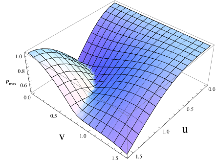
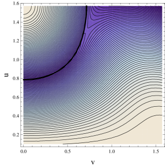
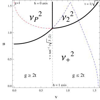
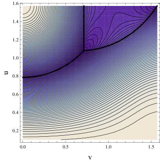
Figure 1: (Color online)
Fig. 1a is a plot of the applicable domains in -plane for .
The principal domain
is located in small and large region. This fact indicates that
this domain is around large region. Fig. 1b is plot of -dependence of
for case. Many highly entangled states are represented as a valley in this
figure. Around and there are a lot of less entangled
states. To compare the applicable domains with we plot both simultaneously in the
plane in Fig. 1c. The black thick line is a boundary between domains. The blue-color
and white-color represent the highly- and less-entangled states respectively. Fig. 1c shows
that the highly-entangled states reside around the boundary between domains.
In this section we would like to compute the geometric entanglement measure defined
(56)
for case. In order to compute we would like to emphasize three points,
which simplify the following calculation. Firstly, note that is given by
(57)
Therefore, we should choose the largest eigenvalue from all eigenvalues, each of which has
its own available regions in the parameter space. Secondly, note that
(58)
This means that is always smaller than in the available region
. Therefore, we can exclude from beginning for the computation
of . Thirdly, note that is obtained from the eigenvalues whose Lagrange
multiplier constants are positiveanalytic .
This fact excludes too. Considering all of these
facts and available regions, it is convenient to divide the whole parameter space into the
following four regions:
(59)
where
(60)
In order to compare with we compute , which is
(61)
where
(62)
Since the last term in , , is non-negative in the region
, both and are non-negative in region III. In region III,
therefore, becomes .
In region II it has been shown in Ref.maximal that when
, where
(63)
Therefore, the region II should be divided into two regions, i.e.
and . Simple consideration shows that when
and when . Combining all of
these facts, one can conclude
(64)
Now, we would like to unify the regions as many as possible to simplify the expression of
. First, one can show that is always non-positive in region A as
following. Since in region A, in this region
(65)
Second, one can show easily that is always non-negative at region D as following.
In this region
(66)
because both terms are non-negative. Combining these facts and Eq.(64) makes
to be expressed as
(69)
In order to understand the behavior of more clearly we introduce the two
parameters and as following:
(70)
with . Then, one can plot the applicable domains
and in the plane, which is Fig. 1a. As Fig. 1a has shown, the domain
for is biased in the small and large region. This indicates that
the domains for is around large region. The remaining region is
the domain for . As will be shown in next section, the number of the
applicable domains for case is not two but three. This means that the phase
factor has great impact in the geometric measure of entanglement.
Fig. 1b is -dependence of given in Eq.(69). At , which means
, becomes because it is separable state. At and , which means
that , becomes again. Between them there is valley, which represents the
set of the highly entangled states. There is different kind of the highly entangled states
around . These highly entangled states are states located near W-state,
.
In order to compare with the applicable domains we plot and the boundary
of domains simultaneously in plane in Fig. 1c. In Fig. 1c the black thick line is a
boundary of the domains. The thick-blue color and light-blue (or white) colors represent the
highly-entangled and less-entangled states, respectively. In the right-upper corner there are
many highly entangled states which are located near W-state. Another type of the
highly entangled states reside near the boundary of the applicable domains. Apart from the
boundary more and more the quantum states lose the entanglement, and eventually reduce to
the separable state.
Now, we consider several special cases. First example is and . In this
case and ,
which gives . Second example is and . In this case
and . Third example is and
. In this case and , which gives
. The second and third examples are consistent with
, where .
Fourth example is case. In this case and
, which results in
(71)
One can show that various limits of Eq.(71) are consistent with the previously
derived results. The last example is case. In this case it is easy to show
(74)
Eq.(74) is perfectly in agreement with the result of Ref.shared .
V Geometric Measure for
In this section we would like to compute the geometric entanglement measure for
case. From the constraint of the positive Lagrange multiplier constant
we can exclude and from beginning stage for the computation of the
geometric measure. Next, we should examine the sign of the Lagrange multiplier
constant for , that is
(75)
It is easy to show that in region. Also it is straightforward
to show that when and when
, where
(76)
Examining Table II and Eq.(76) leads us to divide the whole parameter space into
the following ten regions:
(77)
where
(78)
Figure 2: Pictorial representation for , ,
, and when .
Although the whole space is divided into the ten regions, one can show that some regions do not
exist. In order to show this it is convenient to introduce
(79)
Then, their difference becomes
(80)
Eq.(80) implies that in the region . Then the regions
, , , and
when can be represented as Fig. 2. With an help of Fig. 2 it is easy to
understand that there is no region which satisfies both and
when . This implies that region II and region V do not exist
in the whole parameter space.
In order to compare with we compute , which is
(81)
Therefore, the sign of is determined by . If
, and
(82)
Therefore, if in region, . Thus, we
can exclude in region IV. Similarly, one can show that if in
region, . Therefore, we can exclude
in regions VI and VIII.
Figure 3: Pictorial representation for , ,
, , and
when (Fig. 2 a) and (Fig. 2 b).
Next, we compute , which is
(83)
where
(84)
Direct calculation shows that in region when ,
where
(85)
In addition, simple consideration shows that in region
when and when .
In order to check which eigenvalue is dominant in each region it is convenient to
introduce another parameter
(86)
Then, it is easy to show
(87)
Eq.(87) enables us to represent , ,
, , and
in one-dimensional coordinate, which is illustrated in Fig. 3.
With an help of Fig. 3 one can show
easily that in region III is always non-positive and therefore,
becomes . Using Fig. 3a in region VII is . Using Fig. 3b again
one can show that region IV is divided into
(88)
Finally, we compute , which is
(89)
where
(90)
One can show directly that when . Also, it is
straightforward to show that in region is always smaller than .
Therefore, we can exclude in regions VIII and IX. Combining all of these facts,
one can express for case as follows:
(91)
(94)
(97)
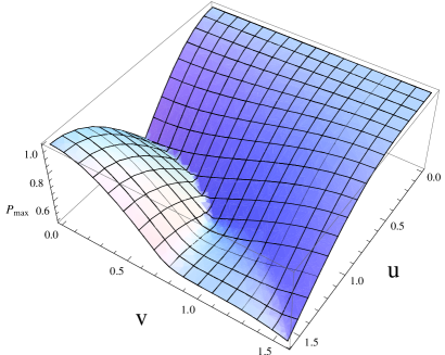
Figure 4: (Color online) Fig. 4(a) is a plot of the applicable domains for
case in -plane. Unlike case there are three applicable domains in this
case. The principal domain is larger than in
case. This fact seems to indicate that the principal domain increases its
territory with increasing . It is important to note that the domain
is not reached to axis. This implies the consistency of the limit.
Fig. 4(b) is -dependence of . The highly entangled states forms a valley
between two mountains. Fig. 4(c) is a plot of and the applicable domains in the
-plane. The boundaries of the domains are represented by black think line. Many
highly-entangles states reside around the boundaries and in the domain . It
is mainly due to the fact that there are two LU-equivalent W-states for case.
Unlike case the whole parameter space is divided into the three applicable
domains. Introducing the parameters and as Eq.(70) we plot the three
applicable domains in the - plane in Fig. 4a. Around axis there are two
domains, i.e. and . Since and go to
and in the limit, this guarantees that the
limit is consistent with same limit of case. The applicable
domain for is little bit larger than the domain for case.
The point () is shared by three domains.
This point corresponds to
(98)
This is LU-equivalent with
as shown in Ref.maximal .
In Fig. 4b we plot the ()-dependence of given in Eq.(91). Like
Fig. 1b the highly entangled states are represented as a valley in this figure. Fig. 4b
seems to show that there exists an alley in the valley, which ends at . Along this
alley so many highly entangled states are located. Comparing Fig. 4b with Fig. 1b, one
can realize that there are many more highly-entangles states for case than
case. This is mainly due to the fact that there are two LU-equivalent
W-states when .
Fig. 4c shows the geometric entanglement measure and the applicable domains simultaneously
in the - plane. Fig. 4c shows that around two W-states there are so many highly
entangled states, which we would like to call W-neighbors. Especially, the neighbors of
in Eq.(98) gather along line. Besides the W-neighbors
there are many highly entangled states around boundary of the applicable domains. These are
the neighbors of the shared statesshared , and we would like to call them
the GHZ-neighbors. The GHZ-neighbors are slightly less-entangled compared to the W-neighbors.
However, the number of the GHZ-neighbors are many more than that of the W-neighbors.
Finally, we consider the several special cases. First example is case. In this case
and , which results in
identical expression with Eq.(74). Therefore, both results for and
cases coincide with each other in the limit. Second example
is case. It is easy to show that in this case when and
when . This is consistent with
when .
VI Eigenvalues and Geometric measure for : Numerical Approach
In this section we will compute the eigenvalues and the geometric measure for
case.
where . From Eq.(102) one can compute if is
known by using
(103)
Deriving from Eq.(102) and inserting it into
Eq.(99c), one can derive the expression of in a form
(104)
On the other hand, one can derive a different expression of directly from
Eq.(102)
(105)
Equating Eq.(104) with Eq.(105) yields an equation for solely :
(106)
where
(107)
Eq.(106) guarantees the existence of the eigenvalue for as
and cases. In fact, one can show that there exists an eigenvalue
corresponding to for arbitrary . We have shown this fact in
appendix A.
Combining Eq.(102) and Eq.(108), the possible solutions for and
are
(109)
It is easy to show that both solutions in Eq.(109) gives a same eigenvalue, which
is
(110)
Finally, let us consider . It is worthwhile noting that at limit
reduces to . Therefore, the
eigenvalues corresponding to should coincide with and
for case, and with and for case at the
limit. Equation gives four solutions of , say
, , and . We ordered the solutions by a fact that
the limit
of and is and same limit of and is
. Then, the corresponding eigenvalues, say , , ,
and , can be computed numerically.
VI.2 geometric measure
Figure 5: (Color online) Fig. 5(a) is a plot of the applicable domains for
case. In this case there are two applicable domains. The principal domain
is little bit larger than for and little bit smaller than
for . This fact indicates that the principal domain increases
its territory with increasing . Fig. 5(b) is -dependence of . As
case the highly-entangled states form a valley between two mountains. Fig. 5(c) is
a plot of and the applicable domains in the -plane. Many highly-entangled
states reside around boundary of the domains and near W-state.
Using eigenvalues , derived analytically and
computed numerically, one can compute for the case. Since each
eigenvalue has its own available region, we checked this region by imposing
, , ,
, and . Although there are six
different eigenvalues, the numerical calculation shows that only and
contribute to the geometric measure. This indicates that the whole parameter space is divided
into two applicable domains. These two domains are represented in plane in Fig. 5a. The
domains is slightly larger than domain and slightly smaller than
domain . This fact seems to indicate that the domain containing extends its
territory with increasing .
Fig. 5b is a -dependence of for . Similarly with
and cases, many highly entangled states reside at the valley between two
mountains. Another highly entangled states reside around , which corresponds to
W-state. The alley appeared in Fig. 4b does not appear in this case. This seems to be due to
the fact that there is only one W-state in case.
Fig. 5c is a -dependence of and domains. As expected the highly entangled
states are located around boundary and W-state.
VII Conclusion
In this paper we have explored the effect of the phase factor in the geometric entanglement
measure. We have chosen the most general three-qubit states which have symmetry under the
qubit-exchange. Our choice of the quantum states enables us to derive all eigenvalues and
geometric measure analytically when the phase factor is or . It turns out
that the case has three applicable domains while the case has two
domains. Most highly entangled states reside around the boundaries of the domains and near
W-state. Apart from the boundaries more and more the quantum states lose their entanglement
and eventually, become the product states.
Our result naturally gives rise to a question:
what is a critical , say ,
which distinguish the two and three domains? In order to explore this question we have
analyzed the case numerically. Our numerical calculation shows that there
are six different eigenvalues for case, but only two of them contribute to
the geometric entanglement measure. Thus, there are two domains for .
We conjecture that emergence of the three applicable domains at is due to
the two LU-equivalent W-states. In order to confirm our conjecture we checked numerically
and cases, which also give two applicable domains. We also
checked the applicable domains for the partially symmetric quantum state
(111)
numerically when . This case also gives two applicable domains. Therefore, we
conclude that the emergence of the three applicable domains is due to the appearance of
additional W-state.
In appendix we have shown that there exist eigenvalues for all , whose Lagrangian
multiplier constant is zero. Although we conjecture that this is due to some symmetry of
the quantum state , we do not know the exact physical reason for the
emergence of these solutions. It seems to be of interest to reveal the physical meaning
of these solutions clearly.
Acknowledgement:
This work was supported by National Research Foundation of Korea Grant funded by the
Korean Government (2009-0073997).
References
(1)R. F. Werner, Quantum states with Einstein-Podolsky-Rosen correlations
admitting a hidden-variable model, Phys. Rev. A 40, 4277(1989).
(2)A. K. Ekert, Quantum cryptography based on Bell’s theorem, Phys. Rev. Lett. 67, 661(1991).
(3) C. H. Bennett and S. J. Wiesner, Communication via one- and
two-particle operators on Einstein-Podolsky-Rosen states, Phys Rev. Lett. 69, 2881(1992).
(4)C. H. Bennett, G. Brassard, C. Crépeau, R. Jozsa, A. Peres, and
W. K.Wootters, Teleporting an unknown quantum state via dual classical and
Einstein-Podolsky-Rosen channels, Phys. Rev. Lett. 70, 1895(1993).
(5)F. Casagrande, A. Lulli, and M. G. A. Paris, Tripartite entanglement
transfer from flying modes to localized qubits, Phys. Rev. A 79, 022307 (2009).
(6)C. H. Bennett, H. J. Bernstein, S. Popescu, and B. Schumacher,
Concentrating partial entanglement by local operations, Phys. Rev. A 53, 2046 (1996).
(7)C. H. Bennett, D. P. DiVincenzo, J. A. Smolin and W. K. Wootters,
Mixed-state entanglement and quantum error correction, Phys. Rev. A 54, 3824(1996).
(8)W. K. Wootters, Entanglement of Formation of an Arbitrary State of
Two Qubits, Phys. Rev. Lett. 80, 2245 (1998).
(9)G. Vidal and J. I. Cirac, Irreversibility in Asymptotic Manipulations
of Entanglement, Phys. Rev. Lett. 86, 5803(2001).
(10)V. Vedral, M. B. Plenio, M. A. Rippin, and P. L. Knight,
Quantifying Entanglement, Phys. Rev. Lett. 78, 2275(1997).
(11)M. B. Plenio and V. Vedral, Bounds on relative entropy of
entanglement for multi-party systems, J. Phys. A: Math. Gen. 34, 6997(2001).
(12)D. A. Meyer and N. R. Wallach, Global entanglement in multiparticle
systems, J. Math. Phys. 43, 4273(2002).
(13)O. Biham, M. A. Nielsen and T. J. Osborne, Entanglement monotone
derived from Grover’s algorithm, Phys. Rev. A 65, 062312(2002).
(14)D. Shapira, Y. Shimoni, and O. Biham, Groverian measure of
entanglement for mixed states, Phys. Rev. A 73, 044301(2006).
(15)A. Shimony, Degree of entanglement, A conference held in honor
of J. A. Wheeler, Ann. N. Y. Acad. Sci.755, 675 (1995).
(16) H. Barnum and N. Linden, Monotones and Invariants for Multi-particle
Quantum States, J. Phys. A: Math.Gen. 34, 6787 (2001).
(17)T.-C. Wei and P. M. Goldbart, Geometric measure of entanglement and
application to bipartite and multipartite quantum states, Phys. Rev. A 68 042307 (2003).
(18)R. Werner and A. Holevo, Counterexample to an additivity conjecture for
output purity of quantum channels, J.Math. Phys. 43, 4353 (2002).
(19) L. Tamaryan, D. K. Park and S. Tamaryan, Generalized Schmidt
Decomposition based on Injective Tensor Norm, [quant-ph/0809.1290].
(20)J. J. Hilling and A. Sudbery, The geometric measure of multipartite
entanglement and the singular values of a hypermatrix, arXiv:0905.2094v2 [quant-ph].
(21)L. Tamaryan, D. K. Park and S. Tamaryan, Analytic Expressions for
Geometric Measure of Three Qubit States, Phys. Rev. A 77 (2008) 022325,
[arXiv:0710.0571 (quant-ph)].
(22)L. Tamaryan, D. K. Park, J. W. Son, and S. Tamaryan, Geometric Measure of
Entanglement and Shared Quantum States, Phys. Rev. A78 (2008) 032304,
[arXiv:0803.1040 (quant-ph)].
(23) E. Jung, M. R. Hwang, D. K. Park, L. Tamaryan and S. Tamaryan, Three-qubit
Groverian Measure, Quant. Inf. Comp. 8 (2008) 0925, [arXiv:0803.3311 (quant-ph)].
(24)Y. Shimoni, D. Shapira, and O. Biham, Characterization of pure quantum states of multiple qubits using the Groverian entanglement measure, Phys. Rev. A 69, 062303 (2004).
(25)M. Hayashi, D. Markham, M. Murao, M. Owari, and S. Virmani, Bounds on Multipartite Entangled Orthogonal State Discrimination Using Local Operations and Classical Communication, Phys. Rev. Lett. 96, 040501 (2006).
(26)O. Gühne, F. Bodoky, and M. Blaauboer, Multiparticle entanglement under the influence of decoherence, Phys. Rev. A 78, 060301(R) (2008).
(27)L. Tamaryan, H. Kim, E. Jung, M.-R. Hwang, D.K. Park, and S. Tamaryan, Toward an understanding of entanglement for generalized n-qubit W-states, arXiv:0806.1314v1[quant-ph].
(28)A. Acín, A. Andrianov, L. Costa, E. Jané, J. I. Latorre, and R. Tarrach, Generalized Schmidt decomposition and classification of three-quantum-bit states, Phys. Rev. Lett. 85, 1560(2000).
(29)H. A. Carteret, A. Higuchi, and A. Sudbery, Multipartite generalisation of the Schmidt decomposition, J. Math. Phys. 41, 7932 (2000).
(30)S. Tamaryan, T. C. Wei and D. K. Park, Maximally entangled three-qubit
states via geometric measure of entanglement, arXiv:0905,3791 (quant-ph).
(31)S.J. van Enk, The joys of permutation symmetry: direct measurements of
entanglement, Phys. Rev. Lett. 102, 190503 (2009).
(32)G. Toth and O. Gühne, Entanglement and permutational symmetry,
Phys. Rev. Lett. 102, 170503 (2009).
(33)T.-C. Wei and S. Severini, Matrix permanent and quantum entanglement of permutation invariant states, arXiv:0905.0012v1 [quant-ph].
Appendix A
In this appendix we would like to show the existence of the eigenvalue , which
corresponds to , at arbitrary . When , Eq.(14)
reduces to
(A.1a)
(A.1b)
(A.1c)
The existence of can be shown as following. First we derive and by
making use of Eq.(A.1a) and Eq.(A.1b). Then we show that the
solutions and also solve Eq.(A.1c).
Now, we consider only case. Then from Eq.(A.1a) and
Eq.(A.1b) it is easy to derive
(A.2)
which gives
(A.3)
Combining Eq.(A.2) and Eq.(A.3), one can derive the solution for ,
which is
(A.4)
Inserting Eq.(A.4) into Eq.(A.1b), one can derive in
a form
(A.5)
Inserting Eq.(A.4) and Eq.(A.5) into the lhs of Eq.(A.1c), one
can show straightforwardly that Eq.(A.1c) is solved already by Eq.(A.4)
and Eq.(A.5). This guarantees the existence of .
In order to derive explicitly we choose the upper sign in Eq.(A.4) and
Eq.(A.5). Then the components of the vector becomes
(A.6a)
(A.6b)
(A.6c)
Inserting Eq.(A.6) into Eq.(4) and performing tedious calculation,
one can show that , eigenvalue corresponding to , becomes
(A.7)
It is straightforward to show that the choice of lower sign in Eq.(A.4) and
Eq.(A.5) leads us to same expression of .
One can show easily that exactly coincides with in Eq.(25),
in Eq.(43) and in Eq.(110) when ,
and respectively.
Finally, making use of explicit expression of , oen can derive the nearest product
state for , i.e.
(A.8)
where is given in Eq.(3). Since is a Bloch vector
of , one can show directly
(A.9)
where
(A.10)
Inserting Eq.(A.9) into Eq.(A.8) it is straightforward to show
that
becomes
(A.11)
where is a normalization constant, which makes unit vector.
For case the nearest product state becomes
(A.12)
It is interesting to note that when , where
is given in Eq.(63).
For case abd becomes
(A.13)
It is interesting to note that when , where
is given in Eq.(85).