Power loss and electromagnetic energy density in a dispersive metamaterial medium
Abstract
The power loss and electromagnetic energy density of a metamaterial consisting of arrays of wires and split-ring resonators (SRRs) are investigated. We show that a field energy density formula can be derived consistently from both the electrodynamic (ED) approach and the equivalent circuit (EC) approach. The derivations are based on the knowledge of the dynamical equations of the electric and magnetic dipoles in the medium and the correct form of the power loss. We discuss the role of power loss in determining the form of energy density and explain why the power loss should be identified first in the ED derivation. When the power loss is negligible and the field is harmonic, our energy density formula reduces to the result of Landau’s classical formula. For the general case with finite power loss, our investigation resolves the apparent contradiction between the previous results derived by the EC and ED approaches.
pacs:
41.20.Jb, 03.50.De, 78.20.CiI Introduction
Artificial electromagnetic media having negative permittivity and permeability have been fabricated and tested experimentally for several years Review . According to Veselago Veselago , these metamaterial media are left-handed (over a finite range of frequency), in the sense that the Poynting vector and wave vector are antiparallel to each other. Besides, they are dispersive and absorptive in general Shelby .
For a dispersive medium with negligible absorption, the energy density formula can be obtained via analyzing an adiabatic electromagnetic process Brillouin ; Landau . However, this analysis does not work when finite absorption is present. To evaluate the electromagnetic energy density stored in a dispersive medium with nonzero absorption, one has to adopt different strategies. Now the existence of the (effective) left-handed metamaterial makes this problem even more dramatic because negative permittivity and permeability seems to imply the possibility of negative energy density, contradicting the thermodynamic stability conditions.
If the absorption of the medium is infinitesimal, the time-averaged energy density of a harmonic electromagnetic wave would be given by Landau :
| (1) |
where and are the complex electric and magnetic fields, and and denote the frequency dependent permittivity and permeability, respectively. Hereafter we name Eq.(1) as Landau’s classical formula. This formula provides a reference for checking the correctness of the desired energy density formula in the lossless limit.
There are two common approaches, namely the equivalent circuit (EC) approach and the electrodynamic (ED) approach, being used to derive the energy density formula for a dispersive media with finite power loss. In the EC approach, firstly one has to transform the wave medium problem to a corresponding electric circuit problem Tretyakov ; Fung , where the values of the capacitances, inductances, resistances and their arrangements in the circuit system can be deduced from the specific forms of and , and then the electric and magnetic energies stored in the circuit system can be evaluated. In the final stage, one transforms the result back to the original wave medium problem to find the corresponding energy density. On the other hand, in the ED approach, the energy density formula is obtained as a byproduct of the following energy conservation law (the Poynting theorem)
| (2) |
This conservation law can be derived using Maxwell’s equations, with the aid of the equations of motions of the polarization and magnetization of the medium Loudon ; Ruppin ; Kong ; Boardman . Here , , and stands for the Poynting vector, energy density, and power loss, respectively. Usually the EC approach provides the time-averaged result although the energy density at a specific time can also be deduced. On the other hand, the ED approach is inherently a time domain approach, which provides the expression of the instantaneous energy density of an arbitrarily varying electromagnetic field. The time-averaged result for a harmonic wave can also be obtained by averaging the energy density in one period of oscillation.
It has been pointed out, if the medium has finite power loss, it is impossible to define the energy density uniquely if we do not have a microstructure model of the material Tretyakov . With the microscopic models of the electric and magnetic constituents of the medium, the dynamical behaviors of the corresponding electric and magnetic dipoles can be predicted, and the energy stored in the the medium can be correctly evaluated. In the literature, several dispersive media with different microscopic dipole models have been considered. The simplest one is an absorptive classical dielectric (Lorentz dispersion) with a single resonant frequency Loudon ; Fung . This can be generalized to the case that both the permittivity and the permeability have Lorentz type dispersions Ruppin ; Kong . Non-Lorentz type dispersions have also been considered. For example, in the wire-SRR metamaterial medium, the wires provide the plasma-like dispersion for permittivity
| (3) |
whereas the SRRs (split-ring resonators) provide a non-Lorentz type dispersion for permeability
| (4) |
Here the parameters and represent the absorption effect of the wires and SRRs, and is a dimensionless factor. Besides, and are the effective plasma frequency of the wire medium and the resonant frequency of the SRR medium, respectively.
Recently, two different expressions for the electromagnetic energy density of the wire-SRR medium were derived using EC Tretyakov and ED Boardman approaches. Although the electric energy densities obtained in these two papers are consistent, their results for the magnetic part are different. In addition, the magnetic energy density formula of Tretyakov (Eq.(31)) does not reduce to the classical result Landau in the lossless limit. We find that this was caused by the fact that in evaluating the total energy (Eq.(27)), the magnetic energy (of form ) stored in the mutual inductance between two sub-circuits was not taken into account by the author. On the other hand, the formula in Boardman (Eq.(19)) does reduce to the classical result in the zero absorption limit. However, when we transform every term in this formula to the corresponding EC system to find its counterpart, an unphysical term (originated from the term in the numerator) appears. Here is the capacitance in the RLC subcircuit of the EC, and is the voltage difference between the two terminals of the resistance in the subcircuit (see Fig.2 of Tretyakov ).
In addition to the above mentioned problems, we also noted that in general the derivation via ED approach does not provide a unique answer. This is caused by the fact that up to now there is no unique way to determine whether a term with the dimension of power should be included in the time derivative of the energy density or in the power loss . In fact, if one does not know the correct form of the power loss, one can always redefine the energy density and power loss as and , where is an arbitrary bilinear function of and . For harmonic and fields, this modification does not change the time-averaged value of (i.e.,), because ( is the period of oscillation). However, usually the time-averaged value of will be modified. This observation explains why the time-averaged power loss formulas obtained in Tretyakov and Boardman are the same, but their time-averaged energy density formulas are different. This observation also reveals that the expression of the energy density is related to the power loss we choose. Note that when we go to the lossless limit, the ambiguity discussed here disappears, and a unique energy density formula can be obtained. However, for the finite loss case, to identify the energy density directly is difficult and we do not know any practical method to avoid the above mentioned ambiguity, thus we propose to identify the power loss first.
In order to resolve the contradictions between the EC and ED approaches and derive a unique and physically reasonable energy density formula, we adopt the following criteria. First, the results derived by using different approaches must be the same. Second, the formula must reduce to Landau’s classical formula in the zero absorption limit. Third, the origin and the expression for the power loss must be carefully analyzed and identified first.
In this paper, we will show that the unique energy density formula can be obtained by using either the ED or EC approach. In addition, the comparison between these two different derivations helps us to clarify the meaning of each physical quantity appearing in the energy density formula. The essential part in the ED derivation is the correct form of the power loss, and we show that it can be found by carefully analyzing the heat generating mechanism in the medium. Our discussion and obtained results in this paper resolve the apparent contradictions between the ED and EC approaches and correct the calculation errors in other previous papers. Although in this paper we consider only the wire-SRR medium, the method is in fact not restricted by this case and can be applied to other kinds of dispersive metamaterial media as well.
This paper is organized as follows. In section II we derive the energy density formula via ED approach. We argue that in this derivation the correct form of power loss is essential for obtaining the unique result we desire. In section III, we further establish the ED-EC correspondence by constructing the EC system for evaluating the magnetic energy stored in the SRR array. The ED-EC correspondence further confirms the correctness of the energy density and power loss formulas obtained by ED approach. In section IV we present the conclusion of this paper.
II Power loss and ED approach
Now we consider the metamaterial medium consisting of metallic wires and split-ring resonators. Under the influence of external electromagnetic field, the wires respond to the field as electric dipoles, whereas the resonators play the role of magnetic dipoles. After averaging the dynamical behavior of these elements, the electromagnetic properties of the medium can be described by an effective theory, having the following macroscopic quantities as dynamical variables: , , , , , . They satisfy the following constituent relations:
| (5) |
| (6) |
The dynamic equations for and are given by
| (7) |
| (8) |
which can be derived by analyzing the currents flowing in the wires and the SRRs under the influence of the applying electromagnetic fields. The displacements of the charges in the wires lead to the electric dipoles, and the total electric dipole moment per unit volume defines the polarization . Therefore, the dynamic equation of follows the form of the equation of motion for the charges. On the other hand, a time varying magnetic field parallel to the axes of the SRR arrays induces the oscillating currents in these SRRs. Suppose the current in an SRR is , and the effective cross section area of it is , then is the magnetic dipole moment of the SRR. The magnetization is then defined by the total magnetic dipole moment per unit volume. The dynamical equation for the currents flowing in the SRRs can be derived by using the Faraday’s law,and the dynamic equation for follows the same form. Note that the term on the right hand side of Eq.(7) is proportional to the electric field , whereas the corresponding term in Eq.(8) is proportional to the time derivative of the magnetic field. This difference is caused by the fact that the electric dipoles are induced by the electric driving field, but the magnetic dipoles in this system can only be induced by the time varying magnetic fluxes through the SRRs. For the details of the derivation, readers may refer to Ref.Pendry1 ; Pendry2 ; Chen . Using Eq.(7) and Eq.(8), and assuming the monochromatic condition, the permittivity of Eq.(3) and permeability of Eq.(4) can be obtained according to the definitions: , .
Now we derive the energy conservation law of the form
| (9) |
from Maxwell’s equations and the dynamical equations of and (Eq.(7) and Eq.(8)). According to Amperé’s law and Faraday’s law, we have
| (10) |
The electric energy density and magnetic energy density can be obtained by integrating the and terms, respectively. The loss term can also be obtained from them. Note that the loss term cannot be written as a total derivative, and this feature was utilized by the authors of Ref.Boardman to find the energy density. However, as we have mentioned before, to uniquely determine the form of the energy density, one has to carefully analyze the origin and the correct form of the power loss first. Once the power loss has been made certain, the energy density can be determined automatically.
The origin and form of the power loss in the wire-SRR medium can be made certain by noticing the following two facts. First, both and are proportional to the currents flowing in the conducting constituents (wires and SRRs) of the wire-SRR medium. Second, the power loss of this medium can only be originated from the Joule heat of form , generated in theses conducting elements. We thus conclude that the power loss of the wire-SRR medium should have the form
| (11) |
where and are two appropriate constants.
Using Eq.(7), we get
| (12) | |||||
thus the electric energy density should be defined as
| (13) |
Note that the additional term in Eq.(12) is the electric part of , consistent with Eq.(11).
The derivation of magnetic energy density is a little different, as will be shown below. Substituting Eq.(8) into the term, we have
| (14) |
The magnetic energy density is thus written as
| (15) |
The term in Eq.(14) represents the magnetic part of the power loss caused by the Joule heat in the split-ring resonators, also consistent with Eq.(11)
Using Eq.(8) once more, the magnetic energy density can be rewritten as
| (16) | |||||
or expressed alternatively as
| (17) | |||||
Note that this final form of magnetic energy density is similar to the Eq.(15) of Boardman , but they are different. Our derivation relies on the knowledge of the correct form of the power loss, whereas the derivation in Boardman did not use this knowledge thus ambiguity may arise as has been explained before.
The total power loss is given by
| (18) |
which is indeed the expected form of Eq.(11), and different from the Eq.(16) of Boardman . Our power loss formula has clear physical meaning, as has been explained before. On the other hand, the Eq.(16) of Boardman has no such clear and convincing meaning, thus we believe it need to be modified. Note that the difference between these two formulas (i.e., ) is given by
| (19) |
Since this is simply a time derivative of a time varying quantity, it contributes nothing to the time-averaged power loss if the field is harmonic. The equivalence relation can be directly checked by explicit calculation.
Now we consider the time averaged energy density for monochromatic wave. Time averaging every term in Eq.(13), we get the electric energy density
| (20) |
Similarly, time averaging all the terms in Eq.(17) and adding them together, we get the magnetic energy density
| (21) |
We stress here that Eq.(21) is just the corrected result of the magnetic energy density formula (31) in Ref.Tretyakov after adding the mutual induction energy term that mentioned in Section I.
III The ED-EC correspondence
Referring to Ref.Chen , we can now construct an EC model for the SRR array. We will show that the magnetic energy density formula (17) can also be derived by virtue of this EC model. The most important distinction between our following derivation and those proposed by others is that we consider arbitrarily varying physical quantities, whereas others considered the restricted harmonic cases. The ED-EC correspondence further confirms the correctness of our derived energy density and power loss formulas.
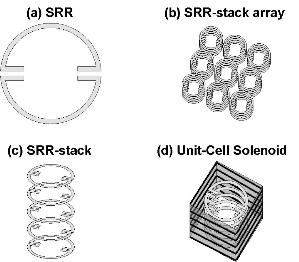
To map the ED quantities to the corresponding EC ones, we adopt the configuration sketched in figure 1. Accordingly, in one unit cell, the SRRs are piled up in the direction to form an SRR-stack, which can be viewed as a circular solenoid. The y-spacing between two successive SRRs in one stack is . These SRR-stacks are periodically arranged at a square lattice of lattice constant . For one unit cell, in order to mimic the magnetic field acting on the SRR-stack inside, we further introduce an imagined cell-solenoid of square cross section, wrapping around the “unit cell tube”. In one turn the coil line of the cell-solenoid is assumed to spiral up in the direction. We will show in the following that by appropriately defining the currents carried by the cell-solenoid and the SRR stack inside the cell tube and the electromotive forces in them, the ED-EC correspondence can indeed be established.
Now we define the physical quantities of the EC system. Since all the vector quantities we considered are parallel to the direction, hereafter we treat them as scalar quantities. The magnetization and the magnetic field (in the connected region outside the SRR stacks) are given by
| (22) |
Here is the filling fraction of the SRR-solenoid in one unit cell.
The magnetic fields outside and inside an SRR-solenoid are
| (23) |
| (24) |
respectively. Here represents the incident magnetic field.
The self inductances per turn of the cell-solenoid and of the SRR-solenoid as well as the mutual inductance between them are given by
| (25) |
The currents flowing in the cell-solenoid () and in the SRR-solenoid () per turn are
| (26) |
The “pure magnetic energy” stored in one slice of the unit cell tube of thickness , without taking into account the energy stored in the interior capacitor of the SRR, can be calculated:
| (27) | |||||
The physical meaning of the last form is obvious since the volume fractions are and , respectively.
The charge and the corresponding energy stored in the interior capacitor of the SRR are
| (28) | |||||
and
| (29) |
respectively. The Joule heat generating in the SRR can also be evaluated:
| (30) |
Here we have used the defining relations Tretyakov :
| (31) |
From these results we conclude that the ED and EC approaches are indeed equivalent. Besides, the physical meaning of each term appearing in Eq.(17) becomes very clear now.
IV Conclusion
In this paper, we review the energy density formulas obtained in Tretyakov and Boardman and analyze the apparent contradictions between the equivalent circuit (EC) and electrodynamics (ED) approach. A small error in the magnetic energy formula of Tretyakov has been pointed out, and the corrected EC energy formula was obtained. We show that energy density of an arbitrarily varying electromagnetic wave in the wire-SRR medium can be derived using either ED or EC approach, and the results are consistent. Besides, our energy density formula reduces to Landau’s classical formula in the lossless limit. This investigation reveals that the ED and EC approaches are equivalent if the correct expression of power loss is known.
Note added. One reviewer of this paper pointed out that in another publication of Prof. Tretyakov’s group Tretyakov1 , the same kind of EC approach as they used in Tretyakov were used again to derive the field energy density. After carefully checking every steps, we found their derivation of magnetic energy formulas (Eq.(28) and Eq.(33)) was based on the Eq.(20), which means the mutual inductance contribution was still omitted. Thus the results in Tretyakov1 should also be corrected. Finally, we must stress that any energy density formula for an effective medium can only be used in the frequency range where the effective theory is accurate enough, and one should not expect the formula to give reliable result beyond this frequency range.
ACKNOWLEDGEMENT
The author gratefully acknowledge financial support from National Science Council (Grant No. NSC 95-2221-E-008-114-MY3) of Republic of China, Taiwan.
References
- (1) Willie J. Padilla, Dimitri N. Basov, David R. Smith, Materials Today 9, 28 (2006).
- (2) V. G. Veselago, Sov. Phys. Usp. 10, 509 (1968)
- (3) R. A. Shelby et al., Science 292, 77 (2001)
- (4) Lon Brillouin, Wave Propagation and Group Velocity (Academic Press, 1960)
- (5) L. D. Landau and E.M. Lifshitz, Electrodynamics of Continuous Media, 2nd. Ed.(Pergamon Press 1984)
- (6) S.A. Tretyakov, Phys. Lett. A, 343, 231 (2005)
- (7) P. C. W. Fung, K. Young, Am J. of Phy., 46, 57 (1978)
- (8) R. Loudon, J. Phys. A: Gen. Phys. 3, 233 (1970)
- (9) R. Ruppin, Phys. Lett. A, 299, 309 (2002)
- (10) Tie Jun Cui, Jin Au Kong, Phys. Rev. B 70, 205106 (2004)
- (11) A. D. Boardman, K. Marinov, Phys. Rev. B 73, 165110 (2006)
- (12) J. B. Pendry, A. J. Holden, W. J. Stewart, I. Youngs, Phys. Rev. Lett. 76, 4773 (1996)
- (13) J. B. Pendry, A. J. Holden, D. J. Robbins, W. J. Stewart, IEEE Trans. Microw. Theory Tech. 47,11 (1999)
- (14) Hongsheng Chen et al., J. Appl. Phys. 100, 024915 (2006)
- (15) P.M.T. Ikonen,S.A. Tretyakov, IEEE Trans. Microw. Theory Tech. 55, 92 (2007)