Stability of Bose-Einstein condensates in a circular array

Abstract

The properties of the superfluid phase of ultra cold bosonic atoms loaded in a circular array are investigated in the framework of the Bose-Hubbard model and the Bogoliubov theory. We derive and solve the Gross-Pitaevskii equation of the model to find that the atoms condense in states of well-defined quasimomentum. A detailed analysis of the coupling structure in the effective quadratic grand-canonical Hamiltonian shows that only pairs of distinct and identical quasimomenta are coupled. Solving the corresponding Bogoliubov-de Gennes equations we see that each pair of distinct quasimomenta gives raise to doublets in the excitation energy spectrum and that the quasimomenta of the zero-energy mode and of the occupied state in the condensates are identical. The dynamical and energetic stabilities of the condensates are determined by studying the behavior of the elementary excitations in the control parameters space. Our investigation establishes that superflow condensates exists only in the central region of the first Brillouin zone whereas there is none in the last quarters since they are energetically unstable, independently of the control parameters.

I Introduction

The experimental realization of Bose-Einstein condensates in a periodic potential created by interference of laser beams, called an optical lattice Raithel ; Muller ; Friebel , opened up the possibility of studying the properties of ultra cold atoms in a variety of conditions. Examples are the access to strongly interacting atomic regimes Chu ; Kasevich and to states which are fundamental for applications in quantum information Jaksch . These systems have proven to be a rich research field that offer the unique possibility to investigate fundamental questions from condensed matter physics to quantum optics.

A Bose-Einstein condensate in an optical lattice is nearly a perfect physical realization of the Bose-Hubbard model, a fact first pointed out by Jaksch and coworkers Jaksch_Bruder . This model gives a description of the physics of interacting bosonic atoms trapped in a lattice potential with atomic tunneling between nearest neighbors and on-site repulsion. The main advantage of these systems is that they are highly controllable. As an example, when the ratio between the interaction and hopping terms is varied by changing the laser intensity, a quantum phase transition from a superfluid phase to a Mott insulator phase is observed Greiner .

In this paper we use the Bose-Hubbard model and the Bogoliubov theory to study the dynamical and energetic stabilities of Bose-Einstein condensates loaded in a periodic ring. The dynamical and energetic stability of condensates in optical lattices have been investigated both theoretically Stringari ; Paraoanu ; Wu ; Machholm ; Modugno and experimentally Fallani ; DeSarlo ; Campbell ; Mun ; Bloch . The purpose of this paper is to give a complete and self-contained description of the properties of condensates, its excitation spectrum and stability. Briefly, we characterize the condensates by the quasimomenta of occupied states which reveals the existence of equilibrium current carrying condensates Paraoanu ; Bloch , we analyze the coupling structure of the effective quadratic grand-canonical Hamiltonian in the quasimomenta basis which allowed us to establish the composition of the elementary excitations, the doublet structure of excitation energy branch and the proper assignment of the zero-energy mode Blaizot and the phonon limit. We find that in the zero-energy mode, which is a direct consequence of the atom number violation by the Bogoliubov theory, the quasimomenta of the atoms are identical to the quasimomentum of the occupied state in the condensate. Turning to the phonon limit we find that it is achieved when the relative quasimomentum $l-p$ goes to zero, with $l$ and $p$ being, respectively, the quasimomenta of the excitation and of the occupied state in the condensate, a fact overlooked in the literature Paraoanu ; Smerzi .

The stability of the condensates is determined by the behavior of the excitation energies and composition of the elementary excitations in the control parameters space. In fact an equilibrium state is dynamically stable if all excitation energies are real, Paraoanu ; Machholm ; Wu ; Modugno , and it is energetically stable if they are positive, Paraoanu ; Fetter ; Machholm ; Modugno . In our study we identify two mechanisms of energetic instability: “crossing” that occurs when the excitation energy vanishes and change its sign and “no-crossing” that occurs when the excitation energy is strictly negative, independently of the control parameters. From this analysis we determine the domains in the control parameters space where it is possible to find metastability in the system, that is, dynamically and energetically stable condensates. Metastable current carrying condensates correspond to local minima of the energy and they are candidates to present superfluid motion Wu ; Bloch .

This paper is organized as follows. In the Section II we derive and solve the Gross-Pitaevskii equation for the Bose-Hubbard model to show that the atoms condense in states with well-defined quasimomentum Paraoanu , revealing the existence of equilibrium current carrying states Bloch . Besides, these states with well-defined quasimomentum define a single-particle basis which diagonalizes the hopping term of the Bose-Hubbard Hamiltonian. In the Section III we determine the energies and the composition of the elementary excitations by the diagonalization of the effective grand-canonical Hamiltonian of the Bogoliubov theory. We express it in the quasimomentum representation to show that only pairs of quasimomenta are coupled. We identify these pairs to cast the effective grand-canonical Hamiltonian into the form of a sum of terms each one involving pairs of identical and distinct quasimomenta. This fact allow us to reduce the process of diagonalization of a $2M\times 2M$ matrix, with $M$ being the number of lattice sites, to one of $2\times 2$ matrices when the quasimomenta of the pairs are identical and $4\times 4$ matrices when they are distinct, which implies that the effective grand-canonical Hamiltonian is diagonal in blocks. In fact, when $M$ is odd, we have $\frac{M-1}{2}$ pairs with distinct quasimomenta and only one pair with identical. On the other hand, for $M$ even, we have $\frac{M}{2}-1$ pairs with distinct quasimomenta and two pairs with identical. We will see that $2\times 2$ blocks correspond to one excitation energy whereas $4\times 4$ blocks correspond to doublets. In the Section IV we determine the dynamical and energetic stability of the condensates by studying the behavior of excitation spectrum and the composition of the elementary excitations in the control parameters space. We found that the stability properties of the condensates depend only on a combination of control parameters $r\equiv\frac{nU}{2J}$, where $n=\frac{N}{M}$, $J$ and $U$ are, respectively, the density of atoms, the hopping and the on-site strenghts. We determine critical values of $r$ that define, in the control parameters space, the domains where it is possible to find superflow states in the system. The dynamical and energetic phase diagrams are shown. A summary and our conclusions are presented in the Section V.

II The Gross-Pitaevskii equation of the Bose-Hubbard model

II.1 The Bose-Hubbard Hamiltonian

The physics of an ultra cold, dilute and interacting Bose gas in a lattice potential is captured by the Bose-Hubbard model Jaksch_Bruder ; Fisher . This model can be seen as an one-mode approximation that involves the states in the first band of the optical lattice. In the tight-binding approximation, the homogeneous Bose-Hubbard Hamiltonian for a system of bosons in a periodic circular array with $M$ sites is given by Paraoanu

$$\hat{H}_{BH}=-J\sum_{\lambda=0}^{M-1}{(\hat{a}_{\lambda}^{\dagger}\hat{a}_{\lambda+1}+\hat{a}_{\lambda+1}^{\dagger}\hat{a}_{\lambda})}+\frac{U}{2}\sum_{\lambda=0}^{M-1}{\hat{n}_{\lambda}(\hat{n}_{\lambda}-1)}.$$ (1)

In (1), $\hat{a}_{\lambda}$ and $\hat{a}_{\lambda}^{\dagger}$ are, respectively, bosonic annihilation and creation operators of atoms on the $\lambda$th lattice site and $\hat{n}_{\lambda}\equiv\hat{a}_{\lambda}^{\dagger}\hat{a}_{\lambda}$ is the atom number operator that counts the number of atoms on the $\lambda$th lattice site. These operators satisfy the periodic boundary condition $\hat{a}_{\lambda}=\hat{a}_{\lambda+M}$. The first term in Bose-Hubbard Hamiltonian is the hopping term that describes the tunnelling of atoms among neighboring lattice sites with hopping strength $J$ and its effect is to delocalize the atoms over the lattice. The second term describes the inter-atomic on-site repulsion with interaction strength $U$ whose effect is to localize the atoms on the sites.

II.2 The condensates

In a condensate all atoms are in the same single-particle state and therefore the many-body state can be written as

$$|c\rangle=\frac{\hat{\Gamma}^{\dagger N}}{\sqrt{N!}}\left|0\right\rangle$$ (2)

where $\hat{\Gamma}^{\dagger}$ is the creation operator of the state occupied by the atoms

$$\hat{\Gamma}^{\dagger}=\frac{1}{\sqrt{N}}\sum_{\lambda=0}^{M-1}{z_{\lambda}\hat{a}_{\lambda}^{\dagger}}$$

which requires that the complex parameters $z_{\lambda}$ must satisfy the constraint

$$\sum_{\lambda=0}^{M-1}{|z_{\lambda}|^{2}}=N.$$ (3)

The parameters $z_{\lambda}$ are determined by a variational principle in which we minimize the mean value of $\hat{H}_{BH}$ in the boson condensate $|c\rangle$, given by (2), subject to the constraint (3). The minimization lead us to the equation

$$-J(z_{\lambda+1}+z_{\lambda-1})+U\left(1-\frac{1}{N}\right)|z_{\lambda}|^{2}z_{\lambda}=\mu z_{\lambda}$$ (4)

which is the Gross-Pitaevskii equation for the Bose-Hubbard model with $\mu$ being the chemical potential. A solution of this equation that satisfy the constraint (3) has the general form

$$z_{\lambda}=\sqrt{\frac{N}{M}}e^{i\theta\lambda}$$

and, from (4), the chemical potential takes the explicit form

$$\mu=-2J\cos\theta+\frac{UN}{M}\left(1-\frac{1}{N}\right).$$ (5)

The possible values of $\theta$ are fixed by the periodic boundary condition $z_{\lambda+M}=z_{\lambda}$ which requires that $\left(e^{i\theta}\right)^{M}=1$. This equation has $M$ solutions which are the $M$th roots of unity, that is, $\theta_{k}=\frac{2\pi k}{M}$ where $k$ is an integer defined on the set $\left\{-\frac{M}{2}+1,\ldots,\frac{M}{2}\right\}$ for $M$ even or $\left\{-\frac{\left(M-1\right)}{2},\ldots,\frac{\left(M-1\right)}{2}\right\}$ for $M$ odd. It follows from all these considerations that the bosonic atoms condense in states with well-defined quasimomentum $\frac{2\pi k}{M}$,

$$\hat{A}_{k}^{\dagger}\equiv\frac{1}{\sqrt{M}}\sum_{\lambda=0}^{M-1}{e^{i\frac{2\pi k}{M}\lambda}\hat{a}_{\lambda}^{\dagger}}.$$ (6)

These states form a single-particle basis which diagonalizes the hopping term of the Bose-Hubbard Hamiltonian. Thus, in this representation, the Hamiltonian (1) has the form

$$\hat{H}_{BH}=\sum_{k}{e_{k}\hat{A}_{k}^{\dagger}\hat{A}_{k}}\\ +\frac{U}{2M}\sum_{\{k_{j}\}}{\delta_{M}(k_{1}+k_{2}-k_{3}-k_{4})\hat{A}_{k_{4}}^{\dagger}\hat{A}_{k_{3}}^{\dagger}\hat{A}_{k_{2}}\hat{A}_{k_{1}}}$$ (7)

where

$$e_{k}\equiv-2J\cos\frac{2\pi k}{M}$$

and the Krönecker modular delta $\delta_{M}\left(k\right)$ is equal to one if $k$ is an integer multiple of $M$ and zero otherwise.

III The elementary excitations

III.1 The effective grand-canonical Hamiltonian and the coupling structure of quasimomenta

To derive the Bogoliubov-de Gennes equations we first define the shifted operators $\hat{c}_{k}$ and $\hat{c}_{k}^{\dagger}$ by

$$\hat{A}_{k}=z_{q}\delta_{k,q}+\hat{c}_{k},$$

where $z_{q}$ is the condensate wave function with quasimomentum $\frac{2\pi q}{M}$. Next we write the zero temperature grand-canonical Hamiltonian $\hat{\Omega}\equiv\hat{H}_{BH}-\mu\hat{N}$, with $\hat{N}$ denoting the number operator, as a normal order expansion with respect to the shifted operators, $\hat{c}_{k}$,

$$\hat{\Omega}=\hat{\omega}_{0}+\hat{\omega}_{1}+\hat{\omega}_{2}+\hat{\omega}_{3}+\hat{\omega}_{4},$$ (8)

where the normal ordered operators $\hat{\omega}_{i}$ involve $i$ shifted operators.

In the Bogoliubov theory the ground state is given by the vacuum of the shifted operators which is a coherent state of the operator $\hat{A}_{k}$. When we calculate the mean value of $\hat{\Omega}$ in this vacuum state it is clear that the only contribution comes from the term $\hat{\omega}_{0}$ whose minimization with respect to $z_{q}$ lead us to equation

$$\left[-2J\cos\frac{2\pi q}{M}+\frac{U}{M}|z_{q}|^{2}-\mu\right]z_{q}=0.$$ (9)

Besides if we calculate the mean value of $\hat{N}$ in this ground state, we get $N=\left|z_{q}\right|^{2}$. Since this equation plus (9) determine $z_{q}$ except by a phase factor, it can be taken as a real parameter. From these considerations it follows that $z_{q}=\sqrt{N}$ and

$$\mu=-2J\cos\frac{2\pi q}{M}+\frac{N}{M}U.$$ (10)

Notice that the expressions (5) and (10), for the chemical potential, coincide in the limit $N\gg 1$.

In the Bogoliubov theory the main hypothesis is that the majority of atoms remains in the boson condensate state and thus the dynamics of the system in the neighborhood of equilibrium states is described by the quadratic term $\hat{\omega}_{2}$ since the equation (9) makes $\hat{\omega}_{1}$ identically zero. Thus, neglecting the third and fourth order terms in (8), we obtain the effective grand-canonical Hamiltonian

$$\hat{\Omega}_{eff}^{(q)}=\hat{\omega}_{0}+\sum_{k}{(\epsilon_{k}^{(q)}+nU)\hat{c}_{k}^{\dagger}\hat{c}_{k}}\\ +\frac{nU}{2}\sum_{k,k^{\prime}}{\delta_{M}(k+k^{\prime}-2q)(\hat{c}_{k}^{\dagger}\hat{c}_{k^{\prime}}^{\dagger}+\hat{c}_{k^{\prime}}\hat{c}_{k})}$$ (11)

where

$$\epsilon_{k}^{\left(q\right)}\equiv e_{k}-e_{q}=2J\left(\cos\frac{2\pi q}{M}-\cos\frac{2\pi k}{M}\right).$$ (12)

The diagonalization of the effective Hamiltonian determines the energies and the composition of the elementary excitations. The non-diagonal term in (11) is the one that creates and annihilates pairs of atoms whose quasimomenta are fixed by the condition $\delta_{M}(k+k^{\prime}-2q)=1$ which is satisfied if $(k+k^{\prime}-2q)$ is an integer multiple of $M$,

$$k+k^{\prime}-2q=\nu\left(q\right)M.$$ (13a)

As the quasimomenta are restricted to the first Brillouin zone, the possible values of $$\nu\left(q\right)$$ are given by

$$\nu\left(q\right)=\begin{cases}\begin{cases}0&\quad\textrm{for }M\textrm{ odd}\\ 0,\>1&\quad\textrm{for }M\textrm{ even}\end{cases}&\qquad\textrm{if }q=0\\ 0,\>-\textrm{sgn}\,q&\qquad\textrm{if }q\neq 0\end{cases}$$ (13b)

where $\textrm{sgn}\,q$ is the signal function which is equal to 1 if $q>0$ and -1 if $q<0$. In the $\nu(q)=0$ equation both quasimomenta are in the first Brillouin zone whereas when $\nu(q)\neq 0$ one of the quasimomenta is outside, the effect of $\nu(q)\neq 0$ is to bring it back to the first Brillouin zone. Notice that, except in the case $q=0$ and $M$ odd, the pairs of quasimomenta coupled in (11) are determined by two equations.

From these equations two properties of the coupling structure of quasimomenta emerge. The first one is the absence of ramifications, that is, one quasimomentum appears only once in the set of pairs satisfying (13a). The second one is that the sets of pairs of quasimomenta obtained from these two equations are disjoint. These considerations indicate that when $M$ is odd, we have $\frac{M-1}{2}$ pairs with distinct quasimomenta and only one pair, $(q,q)$, with identical. On the other hand, for $M$ even, we have $\frac{M}{2}-1$ pairs with distinct quasimomenta and two pairs with identical, $(q,q)$ and $\left(q+\frac{M}{2}\nu(q),q+\frac{M}{2}\nu(q)\right)$, with $\nu(q)=-1$ if $q>0$ and $\nu(q)=1$ if $q\leq 0$. In the Tables 1 and 2, we identify the pairs of quasimomenta coupled in (11) for $M$ even and odd, respectively, irrespective if they differ by an exchange of the quasimomenta.

Table 1: The set of pairs of quasimomenta coupled in the effective grand-canonical Hamiltonian for $M$ even.

$M$ even
$q<0$	$\begin{array}[]{c}\nu(q)=0:\\ \nu(q)=1:\end{array}$	$\begin{array}[]{c}\left(\frac{M}{2}-2|q|-1,-\frac{M}{2}+1\right),\ldots,\left(-|q|,-|q|\right),\ldots,\left(-\frac{M}{2}+1,\frac{M}{2}-2|q|-1\right)\\ \left(\frac{M}{2},\frac{M}{2}-2|q|\right),\ldots,\left(-|q|+\frac{M}{2},-|q|+\frac{M}{2}\right),\ldots,\left(\frac{M}{2}-2|q|,\frac{M}{2}\right)\end{array}$
$q=0$	$\begin{array}[]{c}\nu(0)=0:\\ \nu(0)=1:\end{array}$	$\begin{array}[]{c}\left(\frac{M}{2}-1,-\frac{M}{2}+1\right),\ldots,\left(0,0\right),\ldots,\left(-\frac{M}{2}+1,\frac{M}{2}-1\right)\\ \left(\frac{M}{2},\frac{M}{2}\right)\end{array}$
$q>0$	$\begin{array}[]{c}\nu(q)=0:\\ \nu(q)=-1:\end{array}$	$\begin{array}[]{c}\left(\frac{M}{2},-\frac{M}{2}+2q\right),\ldots,\left(q,q\right),\ldots,\left(-\frac{M}{2}+2q,\frac{M}{2}\right)\\ \left(-\frac{M}{2}+2q-1,-\frac{M}{2}+1\right),\ldots,\left(q-\frac{M}{2},q-\frac{M}{2}\right),\ldots,\left(-\frac{M}{2}+1,-\frac{M}{2}+2q-1\right)\end{array}$

Table 2: The set of pairs of quasimomenta coupled in the effective grand-canonical Hamiltonian for $M$ odd.

$M$ odd
$q<0$	$\begin{array}[]{c}\nu(q)=0:\\ \nu(q)=1:\end{array}$	$\begin{array}[]{c}\left(\frac{M-1}{2}-2|q|,-\frac{M-1}{2}\right),\ldots,\left(-|q|,-|q|\right),\ldots,\left(-\frac{M-1}{2},\frac{M-1}{2}-2|q|\right)\\ \left(\frac{M-1}{2},\frac{M-1}{2}-2|q|+1\right),\ldots,\left(\frac{M-1}{2}-2|q|+1,\frac{M-1}{2}\right)\end{array}$
$q=0$	$\nu(0)=0:$	$\begin{array}[]{c}\left(\frac{M-1}{2},-\frac{M-1}{2}\right),\ldots,\left(0,0\right),\ldots,\left(-\frac{M-1}{2},\frac{M-1}{2}\right)\end{array}$
$q>0$	$\begin{array}[]{c}\nu(q)=0:\\ \nu(q)=-1:\end{array}$	$\begin{array}[]{c}\left(\frac{M-1}{2},-\frac{M-1}{2}+2q\right),\ldots,\left(q,q\right),\ldots,\left(-\frac{M-1}{2}+2q,\frac{M-1}{2}\right)\\ \left(-\frac{M-1}{2}+2q-1,-\frac{M-1}{2}\right),\ldots,\left(-\frac{M-1}{2},-\frac{M-1}{2}+2q-1\right)\end{array}$

III.2 The Bogoliubov-de Gennes equations and elementary excitations

The identification of the pairs of quasimomenta coupled in the effective Hamiltonian shows that it is block diagonal: $2\times 2$ blocks when the quasimomenta of the pairs are identical and $4\times 4$ blocks when they are distinct. In fact, (11) can be cast into the form

$$\hat{\Omega}_{eff}^{(q)}=\sum_{(k,k)}{\hat{h}_{2}(k,k)}+\sum_{{(k,k^{\prime})}\atop{k\neq k^{\prime}}}{{\hat{h}_{2}(k,k^{\prime})}}$$

where the first sum involves pairs with identical quasimomenta while the second distinct, with $\hat{h}_{2}(k,k)$ and $\hat{h}_{2}(k,k^{\prime})$ given explicitly by

$$\hat{h}_{2}(k,k)=(\epsilon_{k}^{(q)}+nU)\hat{c}_{k}^{\dagger}\hat{c}_{k}+\frac{nU}{2}(\hat{c}_{k}^{\dagger}\hat{c}_{k}^{\dagger}+\hat{c}_{k}\hat{c}_{k})$$

and

$$\hat{h}_{2}(k,k^{\prime}) = (\epsilon_{k}^{(q)}+nU)\hat{c}_{k}^{\dagger}\hat{c}_{k}+(\epsilon_{k^{\prime}}^{(q)}+nU)\hat{c}_{k^{\prime}}^{\dagger}\hat{c}_{k^{\prime}}$$

$$+ nU(\hat{c}_{k}^{\dagger}\hat{c}_{k^{\prime}}^{\dagger}+\hat{c}_{k^{\prime}}\hat{c}_{k}).$$

The diagonalization of quadratic Hamiltonians of bosonic operators is a standard problem fully explained in reference Blaizot . In the Appendix A we discuss briefly the procedure of this reference to fix the notation and to present the main properties of the eigenvalue problem. In what follows we will discuss separately the diagonalization of blocks that involve identical and distinct quasimomenta.

• Identical quasimomenta: $2\times 2$ blocks

When $M$ is odd there is only one pair with identical quasimomenta, $(q,q)$, which is equal to the quasimomentum of the occupied state. Solving the corresponding Bogoliubov-de Gennes equations (33) for $\hat{h}_{2}(q,q)$, where $\mathcal{A}=\mathcal{B}=nU$, we find that the eigenmode has zero energy and zero norm. This result is well known and it is a consequence of the broken continuous symmetry which arises due to violation of the atom number conservation by the Bogoliubov theory. In this case $\hat{h}_{2}(q,q)$ can be written as

$$\hat{h}_{2}(q,q)=\frac{\hat{\wp}^{2}}{2\chi}+\frac{nU}{2}$$

where the hermitian operator $\hat{\wp}$ is given by $\frac{1}{\sqrt{2}}(\hat{c}_{q}^{\dagger}+\hat{c}_{q})$ and the inertial parameter $\chi$ is equal to $(2nU)^{-1}$.

On the other hand, when $M$ is even, we found two pairs with identical quasimomenta $(q,q)$ and $\left(q+\frac{M}{2}\nu(q),q+\frac{M}{2}\nu(q)\right)$, with $\nu(q)=-1$ if $q>0$ and $\nu(q)=1$ if $q\leq 0$. The pair with quasimomentum equal to the occupied state, $(q,q)$, gives raise to a zero-energy eigenmode as stated before. In the case of the other pair, $\left(q+\frac{M}{2}\nu(q),q+\frac{M}{2}\nu(q)\right)$, the Bogoliubov-de Gennes equations are given by

$$\left(\begin{array}[]{cc}4J\cos\frac{2\pi q}{M}+nU&nU\\ nU&4J\cos\frac{2\pi q}{M}+nU\end{array}\right)\left(\begin{array}[]{c}u_{q+\frac{M}{2}\nu\left(q\right)}\\ v_{q+\frac{M}{2}\nu\left(q\right)}\end{array}\right)\\ =E_{q+\frac{M}{2}\nu\left(q\right)}^{\left(q\right)}\left(\begin{array}[]{cc}1&0\\ 0&-1\end{array}\right)\left(\begin{array}[]{c}u_{q+\frac{M}{2}\nu\left(q\right)}\\ v_{q+\frac{M}{2}\nu\left(q\right)}\end{array}\right)$$ (14)

where we have used $\epsilon_{q+\frac{M}{2}\nu(q)}^{(q)}=4J\cos\frac{2\pi q}{M}$, from (12) and (13a). Solving these equations we find the excitation energy

$$E_{q+\frac{M}{2}\nu(q)}^{(q)}=\sqrt{4J\cos\frac{2\pi q}{M}\left(4J\cos\frac{2\pi q}{M}+2nU\right)}$$ (15)

and the eigenvectors associated to the pair $\left(E_{q+\frac{M}{2}\nu(q)}^{(q)},-E_{q+\frac{M}{2}\nu(q)}^{(q)}\right)$, $V_{q+\frac{M}{2}\nu(q)}^{(q)}$ and $\gamma V_{q+\frac{M}{2}\nu(q)}^{(q)}$ , respectively, with $V_{q+\frac{M}{2}\nu(q)}^{(q)}=\left(\begin{array}[]{cc}u_{q+\frac{M}{2}\nu(q)}&v_{q+\frac{M}{2}\nu(q)}\end{array}\right)^{T}$, where the symbol $T$ denotes the transpose of the corresponding matrix. As will be clear latter on, another useful quantity is the ratio of the components of the eigenvector given by

$$\frac{v_{q+\frac{M}{2}\nu(q)}}{u_{q+\frac{M}{2}\nu(q)}}=-\frac{\left(4J\cos\frac{2\pi q}{M}+nU-\sqrt{4J\cos\frac{2\pi q}{M}\left(4J\cos\frac{2\pi q}{M}+2nU\right)}\right)}{nU}.$$ (16)

• Distinct quasimomenta: $4\times 4$ blocks

In this case the Bogoliubov-de Gennes equations for $\hat{h}_{2}(k,k^{\prime})$ is given by

$$\left(\begin{array}[]{cccc}\epsilon_{k}^{(q)}+nU&0&0&nU\\ 0&\epsilon_{k^{\prime}}^{(q)}+nU&nU&0\\ 0&nU&\epsilon_{k}^{(q)}+nU&0\\ nU&0&0&\epsilon_{k^{\prime}}^{(q)}+nU\end{array}\right)\left(\begin{array}[]{c}u_{k}\\ u_{k^{\prime}}\\ v_{k}\\ v_{k^{\prime}}\end{array}\right)\\ =E^{(q)}\left(\begin{array}[]{cccc}1&0&0&0\\ 0&1&0&0\\ 0&0&-1&0\\ 0&0&0&-1\end{array}\right)\left(\begin{array}[]{c}u_{k}\\ u_{k^{\prime}}\\ v_{k}\\ v_{k^{\prime}}\end{array}\right).$$ (17)

It is easily seen that equation (17) leaves uncoupled the vectors $V_{I}^{(q)}=\left(\begin{array}[]{cccc}u_{k}&0&0&v_{k^{\prime}}\end{array}\right)^{T}$ and $V_{II}^{(q)}=\left(\begin{array}[]{cccc}0&u_{k^{\prime}}&v_{k}&0\end{array}\right)^{T}$. Therefore this equation can be reduced into two $2\times 2$ eigenvalues equations

$$(I)\left(\begin{array}[]{cc}\epsilon_{k}^{(q)}+nU&nU\\ nU&\epsilon_{k^{\prime}}^{(q)}+nU\end{array}\right)\left(\begin{array}[]{c}u_{k}\\ v_{k^{\prime}}\end{array}\right)\\ =E_{I}^{(q)}\left(\begin{array}[]{cc}1&0\\ 0&-1\end{array}\right)\left(\begin{array}[]{c}u_{k}\\ v_{k^{\prime}}\end{array}\right)$$ (18a)

$$(II)\left(\begin{array}[]{cc}\epsilon_{k^{\prime}}^{(q)}+nU&nU\\ nU&\epsilon_{k}^{(q)}+nU\end{array}\right)\left(\begin{array}[]{c}u_{k^{\prime}}\\ v_{k}\end{array}\right)\\ =E_{II}^{(q)}\left(\begin{array}[]{cc}1&0\\ 0&-1\end{array}\right)\left(\begin{array}[]{c}u_{k^{\prime}}\\ v_{k}\end{array}\right).$$ (18b)

Solving these equations we find that the excitation energies are given by

$$E_{I}^{(q)\pm}=\varepsilon_{A}^{(q)}(k,k^{\prime})\pm\sqrt{\varepsilon_{S}^{(q)}(k,k^{\prime})\left(\varepsilon_{S}^{(q)}(k,k^{\prime})+2nU\right)}$$ (19a)

$$E_{II}^{(q)\pm}=-\varepsilon_{A}^{(q)}(k,k^{\prime})\pm\sqrt{\varepsilon_{S}^{(q)}(k,k^{\prime})\left(\varepsilon_{S}^{(q)}(k,k^{\prime})+2nU\right)}$$ (19b)

where

$$\varepsilon_{A}^{(q)}(k,k^{\prime})\equiv\frac{\epsilon_{k}^{(q)}-\epsilon_{k^{\prime}}^{(q)}}{2},\qquad\varepsilon_{S}^{(q)}(k,k^{\prime})\equiv\frac{\epsilon_{k}^{(q)}+\epsilon_{k^{\prime}}^{(q)}}{2}$$

with $\epsilon_{k}^{(q)}$ given by (12).

Concerning the amplitudes, we found that they satisfy the following relations $u_{k}^{(\pm)}=v_{k}^{(\mp)}$, $u_{k^{\prime}}^{(\pm)}=v_{k^{\prime}}^{(\mp)}$, $u_{k}^{(\pm)}=u_{k^{\prime}}^{(\pm)}$ and $v_{k}^{(\pm)}=v_{k^{\prime}}^{(\pm)}$. These properties allow us to identify two excitation eigenmodes whose pairs of opposite energies are $\left(E_{I}^{(q)+},-E_{I}^{(q)+}=E_{II}^{(q)-}\right)$ and $\left(E_{II}^{(q)+},-E_{II}^{(q)+}=E_{I}^{(q)-}\right)$. The corresponding eigenvectors are $V_{I}^{(q)+}$, $\gamma V_{I}^{(q)+}=V_{II}^{(q)-}$ and $V_{II}^{(q)+}$, $\gamma V_{II}^{(q)+}=V_{I}^{(q)-}$, whose components are $V_{I}^{(q)+}=\left(\begin{array}[]{cccc}u_{k}^{(+)}&0&0&v_{k^{\prime}}^{(+)}\end{array}\right)^{T}$ and $V_{II}^{(q)+}=\left(\begin{array}[]{cccc}0&u_{k^{\prime}}^{(+)}&v_{k}^{(+)}&0\end{array}\right)^{T}$.

Thus, the diagonalization of $4\times 4$ blocks gives raise to doublets of excitation energies which are degenerate when $q=0$ and $q=\frac{M}{2}$, the last one only for $M$ even.

One consequence of the above considerations is that the eigenmodes belonging to a doublet have the same norm, the ratio of the amplitudes given by

$$\frac{v_{k^{\prime}}^{(+)}}{u_{k}^{(+)}}=\frac{v_{k}^{(+)}}{u_{k^{\prime}}^{(+)}}=-\frac{\left(\varepsilon_{S}^{(q)}(k,k^{\prime})+nU-\sqrt{\varepsilon_{S}^{(q)}(k,k^{\prime})\left(\varepsilon_{S}^{(q)}(k,k^{\prime})+2nU\right)}\right)}{nU}.$$ (20)

IV Stability analysis

IV.1 Dynamical stability

According to the Bogoliubov theory an equilibrium state is dynamically stable if all the excitation energies are real. The existence of at least one complex energy is sufficient to guarantee the dynamical instability of the corresponding condensate. In what follows we investigate the dynamical stability of the condensates. We will analyze separately the cases where the quasimomenta of the pair are identical and when they are distinct.

• Pair of identical quasimomenta

As seen in the previous section, for both $M$ odd and even, there is a zero-energy eigenmode with quasimomentum equal to the quasimomentum of the occupied state in the condensate. This is a consequence of the violation of atoms number conservation introduced by the Bogoliubov approach. This mode is always present and leads to an indifferent equilibrium which does not affect the stability of condensates.

For $M$ even there is one more pair of identical quasimomenta equal to $k=q+\frac{M}{2}\nu(q)$, where $\nu(q)=-1$ if $q>0$ and $\nu(q)=1$ if $q\leq 0$. From (15) it follows that the excitation energy is real if one of the conditions

$$\cos\frac{2\pi q}{M}>0$$ (21a)

or

$$\cos\frac{2\pi q}{M}+\frac{nU}{2J}<0$$ (21b)

is obeyed. The condition (21a) is satisfied by the condensates whose quasimomentum of the occupied state is in the interval $0\leq|p|<\frac{\pi}{2}$, with $p\equiv\frac{2\pi q}{M}$, and the condition (21b) is satisfied when the quasimomentum is in interval $\frac{\pi}{2}<|p|\leq\pi$ such that

$$r<-\cos\frac{2\pi q}{M}$$ (22)

where $r$ is the combination of the control parameters $\frac{nU}{2J}$.

Up to now our analysis have established the domain of stability of a particular eigenmode $k=q+\frac{M}{2}\nu(q)$. To establish the dynamical stability of the condensate we have to analyze the behavior of all the doublets in the control parameters space.

• Pair of distinct quasimomenta: the doublets

From (19a) and (19b), the excitation energies of the doublets corresponding to the pair $\left(k,k^{\prime}\right)$ are real if one of the two conditions

$$\varepsilon_{S}^{(q)}(k,k^{\prime})>0$$ (23a)

or

$$\varepsilon_{S}^{(q)}(k,k^{\prime})+2nU<0$$ (23b)

is satisfied, where $\varepsilon_{S}^{(q)}(k,k^{\prime})$ is given explicitly by

$$\varepsilon_{S}^{(q)}(k,k^{\prime}(k))=4J\cos\frac{2\pi q}{M}\sin^{2}\frac{\pi(k-q)}{M}$$ (24)

with $k-q$ assuming the values shown in Table 5.

From (24) it is easily seen that the condition (23a) is satisfied for condensates with quasimomenta defined in the interval $0\leq|p|<\frac{\pi}{2}$. These condensates whose quasimomentum of the occupied state is in the central region of the first Brillouin zone are always dynamically stable, independently of the values of the control parameters. On the other hand the condition (23b) is satisfied for condensates with $\frac{\pi}{2}<|p|\leq\pi$ that obey the inequality

$$r<-\cos\frac{2\pi q}{M}\>\sin^{2}\frac{\pi(k-q)}{M}.$$ (25)

This condition refers to stability of a particular doublet, $(k,k^{\prime}(k))$. However we are interested in establishing a condition that guarantee that the excitation energies of all doublets are real. This requirement is fulfilled if we take the minimum of the right hand side of inequality (25) which, according to Table 5, is achieved when $k-q=\pm 1$. Thus, it follows that the condensates whose quasimomentum of the occupied state is in the last quarters of the first Brillouin zone, $\frac{\pi}{2}<|p|\leq\pi$, are dynamically stable if they obey the condition

$$r<-\cos\frac{2\pi q}{M}\>\sin^{2}\frac{\pi}{M}.$$ (26)

Notice that the stability of the doublets implies the stability of the equal quasimomentum pair since the inequality (22) is contained in (26).

In the Table 3 we summarize our findings and a dynamical stability phase diagram is shown in Figure 1 for $M=5$ sites. We disregard the condensates with quasimomentum $|p|=\frac{\pi}{2}$, the reason being that we cannot find a Bogoliubov transformation that diagonalizes the effective grand-canonical Hamiltonian since all eigenvectors of the Bogoliubov-de Gennes equation have zero norm.

Table 3: Dynamical stability of the condensates.

Dynamical Stability
$0\leq|p|<\frac{\pi}{2}$	always stable
$\frac{\pi}{2}<|p|\leq\pi$	stable if $r<-\cos p\>\sin^{2}\frac{\pi}{M}$

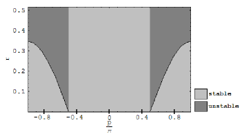
Figure 1: Dynamical stability phase diagram for $M=5$ sites. Notice that $p$ assumes only discrete values $0$, $\pm 0.4\pi$, $\pm 0.8\pi$ indicated in the figure. The condensates with quasimomenta $0$ and $\pm 0.4\pi$, which are in the central region of the first Brillouin zone, are always dynamically stable. On the other hand the dynamical stability of the condensates with quasimomenta $\pm 0.8\pi$, which are in the last quarters of the first Brillouin zone, depends on the control parameters. The continuous curve is only to guide the eye.

When $r=0$ all the condensates are dynamically stable. Actually they are eigenstates of the Bose-Hubbard Hamiltonian when $U=0$. When $r$ starts to increase the condensates with the smallest $|p|$ in the set $\frac{\pi}{2}<|p|\leq\pi$ start to become unstable until $r>\sin^{2}\frac{\pi}{M}$, when all the condensates in the last quarters of the first Brillouin zone are unstable.

Recent experiments Campbell have shown that the onset of dynamical instability occur when two atoms in the condensate can elastically scatter into a final state where they have quasimomenta different from $p=\frac{2\pi q}{M}$. To point out the relevance of our analysis to this matter, we cast the stability condition (23a) into the form Wu

$$2e_{q}<e_{k}+e_{k^{\prime}}.$$ (27)

This condition reveals that in the condensates whose quasimomentum of the occupied state is in the central region of the first Brillouin zone, pairs of atoms cannot elastically scatter into two different quasimomentum states $\frac{2\pi k}{M}$ and $\frac{2\pi k^{\prime}}{M}$.

For the condensates whose quasimomentum of the occupied state is in the last quarters of the first Brillouin zone the stability condition (23b) takes the form

$$2e_{q}>e_{k}+e_{k^{\prime}}+2nU.$$ (28)

Notice that in this case the quantity $2e_{q}-e_{k}-e_{k^{\prime}}$ is positive and has a lower limit equal to $2nU$ which implies that two atoms can inelastically scatter with the excess of energy being transferred to the other atoms in the system. However, notice that in the thermodynamical limit all these condensates are dynamically unstable.

IV.2 Energetic stability

In the framework of the Bogoliubov theory an equilibrium state is energetically unstable if there is at least one negative excitation energy. Recall that to an elementary excitation we associate a pair of eigenvectors with opposite eigenvalues $(E,-E)$ and opposite sign of the norm, where the value of the excitation energy is the eigenvalue of the eigenvector with a positive norm.

We can distinguish two mechanisms of energetic instability. One is “crossing” that occurs when a positive excitation energy vanishes and changes the sign and the second is “no-crossing” where we always have a negative excitation energy. The difference between these two mechanisms is that “crossing” depends on the control parameters whereas “no-crossing” does not.

We restrict our analysis of energetic stability to dynamically stable condensates whose excitation energies are all real, a necessary condition of energetic stability. Our procedure to establish the energetic stability of the condensates is, for each eigenmode, to identify the eigenvector with positive norm and the sign of the corresponding eigenvalue. The sign of the norm depends on the size of the ratio $\frac{v}{u}$. If $0<\left|\frac{v}{u}\right|<1$ the norm is positive and if $\left|\frac{v}{u}\right|>1$ the norm is negative. Following what we have done in the case of dynamical stability, we will discuss separately the case of identical and distinct pairs of quasimomenta.

• Pair of identical quasimomenta

As pointed out before the zero-energy eigenmode does not affect the stability of the condensates. Therefore we are left with the pair $k=q+\frac{M}{2}\nu(q)$, with $\nu(q)=-1$ if $q>0$ and $\nu(q)=1$ if $q\leq 0$, that exists only for $M$ even. By inspection of the equation (16) we find that

a) if $\cos\frac{2\pi q}{M}>0$, then $V_{q+\frac{M}{2}\nu(q)}^{(q)}$ has a positive norm;

b) if $\cos\frac{2\pi q}{M}+\frac{nU}{2J}<0$, then $V_{q+\frac{M}{2}\nu(q)}^{(q)}$ has negative norm.

Since in both cases the corresponding energy $E_{q+\frac{M}{2}\nu(q)}^{(q)}$ is always positive we conclude that in case a), where $0\leq|p|<\frac{\pi}{2}$, this particular eigenmode is always energetically stable. On the other hand, in case b), where $\frac{\pi}{2}<|p|\leq\pi$, it is always energetically unstable.

• Pair of distinct quasimomenta: the doublets

Inspection of equation (20) shows that,

a) if $\varepsilon_{S}^{(q)}(k,k^{\prime})>0$, then $V_{I}^{(q)+}$ and $V_{II}^{(q)+}$ have positive norm;

b) if $\varepsilon_{S}^{(q)}(k,k^{\prime})+2nU<0$, then $V_{I}^{(q)+}$ and $V_{II}^{(q)+}$ have negative norm.

Notice from (19a) and (19b) that the sign of the energies $E_{I}^{(q)+}$ and $E_{II}^{(q)+}$ depends on the term $\varepsilon_{A}^{(q)}(k,k^{\prime})$, given explicitly by

$$\varepsilon_{A}^{(q)}(k,k^{\prime}(k))=2J\sin\frac{2\pi q}{M}\sin\frac{2\pi(k-q)}{M}$$ (29)

for all the pairs of quasimomenta $(k,k^{\prime}(k))$. According to Table 5, we see that this term is semi-negative definite,

$$\varepsilon_{A}^{(q)}(k,k^{\prime}(k))\leq 0.$$

This property implies that $E_{II}^{(q)+}$ is always positive, whereas $E_{I}^{(q)+}$ can change its sign.

In the case a), where $p$ is defined in the range $0\leq|p|<\frac{\pi}{2}$, the condition for the $(k,k^{\prime}(k))$ mode to be energetically stable is $E_{I}^{(q)+}>0$ which can be cast into the form

$$\varepsilon_{S}^{(q)}(k,k^{\prime})\left(\varepsilon_{S}^{(q)}(k,k^{\prime})+2nU\right)-\left[\varepsilon_{A}^{(q)}(k,k^{\prime})\right]^{2}>0.$$

Inserting the expressions (24) and (29) in the above inequality we obtain

$$\cos^{2}\frac{2\pi q}{M}+r\cos\frac{2\pi q}{M}>\cos^{2}\frac{\pi(k-q)}{M}.$$

However we are interested in a condition that guarantee the stability of all the doublets. This requirement is satisfied if we take the maximum of the right hand side, which is achieved at $k-q=\pm 1$. Thus, the condensates such that $0\leq|p|<\frac{\pi}{2}$ are energetically stable if they obey the condition

$$\cos^{2}\frac{2\pi q}{M}+r\cos\frac{2\pi q}{M}>\cos^{2}\frac{\pi}{M},$$

which can be written in a more convenient way as

$$\sin\left(\frac{2\pi q}{M}-\frac{\pi}{M}\right)\sin\left(\frac{2\pi q}{M}+\frac{\pi}{M}\right)<r\cos\frac{2\pi q}{M}.$$ (30)

Thus, in this case, the route to energetic instability is the “crossing” mechanism.

In the case b) where the condensates are such that $\frac{\pi}{2}<|p|\leq\pi$, one of the energies of the doublets are always negative. To see this, note that $E_{II}^{(q)+}$ is always positive and the corresponding eigenvector, $V_{II}^{(q)+}$ , has negative norm. Thus, by the Bogoliubov criteria, the excitation energy of this mode is $-E_{II}^{(q)+}=E_{I}^{(q)-}$ which is strictly negative, independently of the control parameters. Therefore, we conclude that the condensates whose quasimomentum of the occupied state is in the last quarters of the first Brillouin zone are always energetically unstable, in this case through the “no-crossing” mechanism. In the Table 4 we summarize our findings.

Table 4: Energetic stability of condensates.

Energetic Stability
$0\leq|p|<\frac{\pi}{2}$	stable if $\sin\left(p-\frac{\pi}{M}\right)\sin\left(p+\frac{\pi}{M}\right)<r\cos p$
$\frac{\pi}{2}<|p|\leq\pi$	always unstable

In the Figure 2 we present the energetic stability phase diagram for $M=5$ sites and in the thermodynamical limit, $M\gg 1$, $n=\frac{N}{M}$ fixed. We plot the curve that defines the boundary of energetic stability only for $r\geq 0$. This curve is confined in the central region of the first Brillouin zone where the condensates are always dynamically stable, independently of the control parameters. In the last quarters, the condensates are always energetically unstable.

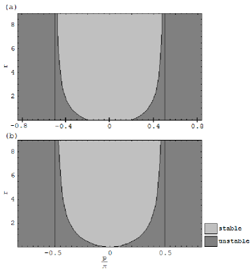
Figure 2: Energetic stability phase diagram (a) for $M=5$ sites and (b) in the thermodynamical limit $M\gg 1$, $n=\frac{N}{M}$ fixed. In (a), since $r$ is a semi-positive definite parameter, we did not plot the curve that defines the boundary of energetic stability in the interval $0\leq|p|\leq\frac{\pi}{M}$ where $r$ is negative. Notice that, in (a), $p$ assumes only discrete values $0$, $\pm 0.4\pi$, $\pm 0.8\pi$ indicated in the figure and the continuous curve is only to guide the eye. The two vertical continuous lines define the region where the condensates are always dynamically stable, independently of control parameters.

One question that we can address is to determine the interval of control parameters in which there are metastable current carrying condensates, that is, dynamically and energetically stable condensates where the occupied states have a finite quasimomentum. These superflow states correspond to local minima of the energy and they are candidates to present superfluid motion. To find this interval notice that we can define a critical value $r$, say $r_{\textrm{st}}$, such that for $r\geq r_{\textrm{st}}$ the condensates with $0<|p|<\frac{\pi}{2}$ are all metastable. If $p_{\textrm{max}}$ is the highest value of $p$ defined in the interval $0<|p|<\frac{\pi}{2}$, from (30) the critical value $r_{\textrm{st}}$ is given explicitly by

$$r_{\textrm{st}}=\frac{\sin\left(p_{\textrm{max}}-\frac{\pi}{M}\right)\sin\left(p_{\textrm{max}}+\frac{\pi}{M}\right)}{\cos p_{\textrm{max}}}.$$ (31)

We can also define another critical value $r$, say $r_{\textrm{unst}}$, such that for $r<r_{\textrm{unst}}$ there is no metastability. When this occur only the $p=0$ condensate is stable. From this consideration follows that

$$r_{\textrm{unst}}=\frac{\sin\left(p_{\textrm{min}}-\frac{\pi}{M}\right)\sin\left(p_{\textrm{min}}+\frac{\pi}{M}\right)}{\cos p_{\textrm{min}}}.$$

Since $\left|p_{\textrm{min}}\right|=\frac{2\pi}{M}$, $r_{\textrm{unst}}$ is given by

$$r_{\textrm{unst}}=\frac{\sin\left(\frac{3\pi}{M}\right)\sin\left(\frac{\pi}{M}\right)}{\cos\frac{2\pi}{M}}.$$ (32)

When $r$ increases continuously from zero there is a hierarchy in the appearance of these superflow states, starting at $r=r_{\textrm{unst}}$ where pairs of degenerate condensates with quasimomentum $p$ and $-p$, beginning with $p=\frac{2\pi}{M}$, become metastable up to $r\geq r_{\textrm{st}}$ when all states are metastable.

V Summary and conclusions

In this paper we use the Bose-Hubbard model and the Bogoliubov theory to investigate the properties of ultra cold bosonic atoms loaded in a periodic ring with $M$ sites. First we derive and solve the Gross-Pitaevskii equation of the model and from the analysis of the solutions we show that the atoms condense in states with well-defined quasimomentum whose values are the $M$th roots of unit, restricted to the first Brillouin zone. Thus, besides the usual zero quasimomentum condensate, we have equilibrium states with non-zero quasimomentum which correspond to current carrying condensates Bloch . These states with well-defined quasimomentum form a basis that diagonalize the hopping term of the Bose-Hubbard Hamiltonian.

Following the Bogoliubov theory we derive the effective grand-canonical Hamiltonian, quadratic in the shifted operators, whose diagonalization gives the energies and the composition of the elementary excitations. A detailed analysis of the coupling structure in the effective grand-canonical Hamiltonian shows that only pairs of identical and distinct quasimomenta are coupled. An immediate consequence of this coupling structure is that the effective Hamiltonian is block diagonal: $2\times 2$ blocks when the quasimomenta of the pairs are identical and $4\times 4$ blocks when they are distinct. The diagonalization of the $2\times 2$ blocks shows that the pair $(q,q)$ with quasimomentum equal to the quasimomentum of the occupied state in the condensate gives raise to the zero-energy eigenmode. On the other, the diagonalization of the $4\times 4$ blocks gives raise to doublets of excitation energies which are degenerate when $q=0$ and, for $M$ even, $q=\frac{M}{2}$. This shows that when $q\neq 0$ the excitation spectrum has a two-branch structure. We have also found, by inspection of the excitation energies (19a) and (19b), that the phonon limit is achieved when the relative quasimomentum $l-p$ goes to zero, with $l=\frac{2\pi k}{M}$ being the quasimomentum of the excitation. Indeed, in this limit it follows that $E_{I,II}=c_{I,II}|l-p|$ with two different sound velocities: $c_{I}^{+}=2J(-\sin p+\sqrt{r\cos p})$ and $c_{II}^{+}=2J(\sin p+\sqrt{r\cos p})$. These properties are signatures of the finite size of the quasimomentum of the occupied state in the condensates.

Our stability analysis shows that the condensates in the central region of the first Brillouin zone, $0\leq|p|<\frac{\pi}{2}$, are always dynamically stable whereas the dynamical stability of the condensates in the last quarters, $\frac{\pi}{2}<|p|\leq\pi$, depends on the control parameters. When $r$ increases from zero, these condensates start to become unstable beginning with the one of smallest $|p|$ ending up with the instability of all condensates, when $r>\sin^{2}\frac{\pi}{M}$.

Concerning the energetic stability, we found that the condensates in the last quarters of the first Brillouin zone are always unstable whereas the energetic stability of the condensates in the central region depends on the control parameters. We show that when $r<r_{\textrm{unst}}$ only the $p=0$ condensate is stable. However, when $r>r_{\textrm{unst}}$, pairs of degenerate condensates with non-zero quasimomentum, $p$ and $-p$, start to become energetically stable ending up with all the condensates in the central region of the first Brillouin zone being energetically stable, when $r>r_{\textrm{st}}$.

As discussed in the paper, metastable current carrying condensates are candidates to present superfluid motion. A metastable state is both dynamically and energetically stable, consequently a local minimum of the energy. Our analysis shows that the Bogoliubov theory predicts that there is an interval in the control parameters space where metastable current carrying condensates exist. The number of these states increases with $r$ and they are restricted to the central region of the first Brillouin zone.

Appendix A The diagonalization of a quadratic Hamiltonian of bosonic operators

A general quadratic Hamiltonian of bosonic operators is given by

$$\hat{H}=\sum_{i,j}{\mathcal{A}_{ij}\hat{c}_{i}^{\dagger}\hat{c}_{j}}+\frac{1}{2}\sum_{i,j}{(\mathcal{B}_{ij}\hat{c}_{i}^{\dagger}\hat{c}_{j}^{\dagger}+\mathcal{B}_{ij}^{\star}\hat{c}_{j}\hat{c}_{i})}$$

where $\hat{c}_{i}^{\dagger}$ and $\hat{c}_{i}$ are creation and annihilation bosonic operators, $\mathcal{A}_{ij}$ and $\mathcal{B}_{ij}$ are elements of an hermitian and symmetric matrices, respectively. The diagonalization of this quadratic Hamiltonian consists in finding a canonical transformation to quasiparticle operators,

$$\hat{b}_{n}^{\dagger}\equiv\sum_{r}{(u_{r}^{n}\hat{c}_{r}^{\dagger}-v_{r}^{n}\hat{c}_{r})},$$

such that $\hat{H}$, when written in terms of this operators, takes the form of a system of non-interacting quasiparticles. From this constraint it follows that

$$\left(\begin{array}[]{cc}\mathcal{A}&\mathcal{B}\\ \mathcal{B}^{\star}&\mathcal{A}^{\star}\end{array}\right)\left(\begin{array}[]{c}u^{n}\\ v^{n}\end{array}\right)=E_{n}\left(\begin{array}[]{cc}1&0\\ 0&-1\end{array}\right)\left(\begin{array}[]{c}u^{n}\\ v^{n}\end{array}\right)$$ (33)

which is the matrix form of Bogoliubov-de Gennes equations that determines the excitation energies $E_{n}$ and the composition of the elementary excitations $V^{n}=\left(\begin{array}[]{cc}u^{n}&v^{n}\end{array}\right)^{T}$, with $T$ denoting the transpose of the corresponding matrix. When the eigenvalues $E_{n}$ are real, they appear in pairs $\left(E_{n},-E_{n}\right)$ with opposite sign of the norm, $\sum_{r}{(|u_{r}^{n}|^{2}-|v_{r}^{n}|^{2})}$. In fact, if $V^{n}$ is an eigenvector with the eigenvalue $E_{n}$ then $\gamma V^{n\star}$, with

$$\gamma\equiv\left(\begin{array}[]{cc}0&1\\ 1&0\end{array}\right),$$

is an eigenvector with the opposite eigenvalue, $-E_{n}$, and opposite sign of the norm. The excitation energy is identified with the eigenvalue whose eigenvector has a positive norm.

Appendix B Parametrization of the pairs of distinct quasimomenta

As seen before the pairs of distinct quasimomenta, $\left(k,k^{\prime}\right)$, coupled in the effective grand-canonical Hamiltonian identify the doublets that compose the excitation spectrum of the condensates. However $k$ and $k^{\prime}$ are not independent since they are related by equation (13a). Therefore we need one parameter to identify the doublets. Our choice was the relative quasimomentum, $\frac{2\pi}{M}(k-q)$, which leads to an ordered and one-to-one parametrization of the doublets. This can be easily seen noticing that we can cast the equation (13a) into the form

$$(k-q)+(k^{\prime}-q)=\nu\left(q\right)M,$$

and, from it, follows the parametrization shown in the Table 5.

Table 5: Identification of the doublets in the excitation spectrum by the relative quasimomenta $\frac{2\pi}{M}(k-q)$ of the atoms in the condensate.

Condensate	Doublets ($k-q$)
	$M$ odd	$M$ even
$q\leq 0$	$1\leq k-q\leq\frac{M-1}{2}$	$1\leq k-q\leq\frac{M}{2}-1$
$q>0$	$-\frac{M-1}{2}\leq k-q\leq-1$	$-\frac{M}{2}+1\leq k-q\leq-1$

This parametrization can be extended to include the pairs of identical quasimomenta. Indeed, $k-q=0$ for the $(q,q)$ pair and $k-q=\nu(q)\frac{M}{2}$ for the $\left(q+\nu(q)\frac{M}{2},q+\nu(q)\frac{M}{2}\right)$ pair.

References

- (1) G. Raithel, G. Birkl, A. Kastberg, W. D. Phillips and S. L. Rolston, Phys. Rev. Lett. 78, 630 (1997)
- (2) T. Müller-Seydlitz, M. Hartl, B. Brezger, H. Hänsel, C. Keller, A. Schnetz, R. J. C. Spreeuw, T. Pfau and J. Mlynek, Phys. Rev. Lett. 78, 1038 (1997)
- (3) S. Friebel, C. D’Andrea, J. Walz, M. Weitz and T. W. Hänsch, Phys. Rev. A 57, R20 (1997)
- (4) S. Chu, Nature (London), 416, 206 (2002)
- (5) C. Orzel, A. K. Tuchman, M. L. Fenselau, M. Yasuda and M. A. Kasevich, Science 291, 2386 (2001)
- (6) D. Jaksch, Cont. Phys. 45, 367 (2004)
- (7) D. Jaksch, C. Bruder, J. I. Cirac, C. W. Gardiner and P. Zoller, Phys. Rev. Lett. 81, 3108 (1998)
- (8) M. Greiner, M. O. Mandel, T. Esslinger, T. Hänsch and I. Bloch, Nature 415, 39 (2002)
- (9) G. Orso, C. Menotti and S. Stringari, Phys. Rev. Lett. 97, 190408 (2006)
- (10) Gh.-S. Paraoanu, Phys. Rev. A 67, 023607 (2003)
- (11) B. Wu and Q. Niu, Phys. Rev. A 64, 061603 (2001)
- (12) M. Machholm, C. J. Pethick, and H. Smith, Phys. Rev. A 67, 053613 (2003)
- (13) M. Modugno, C. Tozzo and F. Dalfovo, Phys. Rev. A 70, 043625 (2004)
- (14) L. Fallani, L. De Sarlo, J. E. Lye, M. Modugno, R. Saers, C. Fort and M. Inguscio, Phys. Rev. Lett. 93, 140406 (2004)
- (15) L. De Sarlo, L. Fallani, J. E. Lye, M. Modugno, R. Saers, C. Fort and M. Inguscio, Phys. Rev. A 72, 013603 (2005)
- (16) G. K. Campbell, J. Mun, M. Boyd, E. W. Streed, W. Ketterle and D. E. Pritchard, Phys. Rev. Lett. 96, 020406 (2006)
- (17) J. Mun, P. Medley, G. K. Campbell, L. G. Marcassa, D. E. Pritchard and W. Ketterle, Phys. Rev. Lett. 99, 150604 (2007)
- (18) I. Bloch, J. Dalibard and W. Zwerger, Rev. Mod. Phys. 80, 885 (2008)
- (19) J. P. Blaizot and G. Ripka, Quantum Theory of Finite Systems (Cambridge, MA: MIT Press, 1986)
- (20) A. Smerzi, A. Trombettoni, arXiv:0801.4909v1
- (21) A. A. Svidzinsky and A. L. Fetter, Phys. Rev. Lett. 84, 5919 (2000)
- (22) M. P. A. Fisher, P. B. Weichman, G. Grinstein and D. S. Fisher, Phys. Rev. B 40, 546 (1989)