Rabi Interferometry and Sensitive Measurement
of the Casimir-Polder Force with Ultra-Cold Gases

Abstract

We show that Rabi oscillations of a degenerate fermionic or bosonic gas trapped in a double-well potential can be exploited for the interferometric measurement of external forces at micrometer length scales. The Rabi interferometer is less sensitive, but easier to implement, than the Mach-Zehnder since it does not require dynamical beam-splitting/recombination processes. As an application we propose a measurement of the Casimir-Polder force acting between the atoms and a dielectric surface. We find that even if the interferometer is fed with a coherent state of relatively small number of atoms, and in the presence of realistic experimental noise, the force can be measured with a sensitivity sufficient to discriminate between thermal and zero-temperature regimes of the Casimir-Polder potential. Higher sensitivities can be reached with spin squeezed states.

Introduction. Interferometers with trapped ultra-cold atoms are valuable tools for the precise measurement of external forces Cronin et al. (2009). A promising one is the double-well Mach-Zehnder interferometer (MZI) Pezzé et al. (2005); Lee (2006); Huang and Moore (2008); Jo et al. (2007); Schumm et al. (2005); Gati et al. (2006); Böhi et al. (2009). This requires two 50/50 beam splitters implemented by a dynamical manipulation of the inter-well barrier. The phase shift is accumulated during the interaction of atoms with an external potential in the absence of the inter-well coupling. It is interesting to search for alternative interferometric schemes which can be easier to realize and therefore can be more stable than the MZI. In this Letter we propose a new protocol to create a Rabi interferometer. It can be implemented using either degenerate spin-polarized Fermions or non-interacting Bose-Einstein condensates (BECs) trapped in a double-well potential. The gas tunnels between the two wells while acquiring, at the same time, a phase shift. The relative number of particles among the two wells undergoes Rabi oscillations analogous to those experienced by a collection of two-level atoms in a radio frequency field Windpassinger et al. (2008). The measurement of population imbalance as a function of time allows to infer the value of the external force as it affects both the amplitude and frequency of Rabi oscillations. The Rabi interferometer is less sensitive than the MZI, but does not require any splitting/recombination processes and is suitable for the estimation of forces rapidly decaying with distance. In particular, once fed with a fermionic/bosonic spin coherent state, the interferometer allows for the accurate measurement of the Casimir-Polder force between the atomic sample and a surface. We show that even in the presence of typical experimental noise it is possible to distinguish between thermal and zero-temperature regimes of the Casimir-Polder potential Antezza et al. (2004), which has not yet been achieved in experiment Pasquini et al. (2004); Harber et al. (2005); ju Lin et al. (2004); Obrecht et al. (2007); Sukenik et al. (1993). Moreover, we demonstrate that the Rabi interferometer can further benefit from the use of entangled states as input. In analogy to the MZI, a sub shot-noise phase sensitivity can be obtained with spin squeezed states recently created with a BEC Esteve et al. (2008).

The Rabi interferometer. Let us consider a degenerate gas of non-interacting atoms confined in a double-well potential along the $x_{1}$ direction, and in a harmonic trap along $x_{2}$ and $x_{3}$. A field operator formalism allows for studying interferometry with both bosons and fermions. We introduce the field operator $\hat{\Psi}(\vec{r})=\sum_{\vec{k}}\psi_{k_{1}}(x_{1})\psi_{k_{2}}(x_{2})\psi_{k_{3}}(x_{3})\,\hat{c}_{\vec{k}}$, where $\psi_{k_{i}}(x_{i})$ are single-particle energy eigenfunctions along the $i$-th direction and the sum is over the complete set of quantum numbers $\vec{k}\equiv(k_{1},k_{2},k_{3})$. The annihilation (creation) operators $\hat{c}_{\vec{k}}$ ($\hat{c}_{\vec{k}}^{\dagger}$) satisfy commutation or anticommutation relations, depending on the statistics. In two-mode approximation (taking into account only lowest $k_{1}=0$ and the first excited $k_{1}=1$ states) we introduce the wave functions $\psi_{a/b}(x_{1})=(\psi_{0}(x_{1})\pm\psi_{1}(x_{1}))/\sqrt{2}$ and mode operators $\hat{a}_{\vec{k}_{\perp}}=(\hat{c}_{0,\vec{k}_{\perp}}+\hat{c}_{1,\vec{k}_{\perp}})/\sqrt{2}$ and $\hat{b}_{\vec{k}_{\perp}}=(\hat{c}_{0,\vec{k}_{\perp}}-\hat{c}_{1,\vec{k}_{\perp}})/\sqrt{2}$, where $\vec{k}_{\perp}\equiv(k_{2},k_{3})$. The dynamics of the system is thus governed by the Hamiltonian

$$\hat{H}=-E_{J}\hat{J}_{x}+\delta\hat{J}_{z},$$ (1)

where $E_{J}$ is the tunneling energy, $\delta$ is the relative energy shift due to interaction with a position-dependent external potential $V(x_{1})$ not (a). The operators $\hat{J}_{x}$, $\hat{J}_{y}$ and $\hat{J}_{z}$ not (b) form a closed algebra of angular momentum. The goal of the Rabi interferometer is to estimate $\delta$ with the highest possible sensitivity. We consider the measurement of the population imbalance between the two modes, which can be expressed in terms of the eigenvalues of the operator $\hat{J}_{z}$. Using the evolution operator generated by (1),

$$\hat{U}(t)=e^{-i\alpha\hat{J}_{y}}e^{i\Omega\hat{J}_{x}}e^{i\alpha\hat{J}_{y}},$$ (2)

we obtain $\hat{J}_{z}(t,\delta)=u(t,\delta)\hat{J}_{x}+v(t,\delta)\hat{J}_{y}+w(t,\delta)\hat{J}_{z}$, with $u(t,\delta)=\sin\alpha\cos\alpha(\cos\Omega-1)$, $v(t,\delta)=-\cos\alpha\sin\Omega$ and $w(t,\delta)=(\cos^{2}\alpha\cos\Omega+\sin^{2}\alpha)$. Here, $\Omega=\omega t$, $\cos\alpha=E_{J}/\hbar\omega$, $\sin\alpha=\delta/\hbar\omega$ and $\omega=\sqrt{E_{J}^{2}+\delta^{2}}/\hbar$ is the detuned Rabi frequency.

The estimation protocol consists of measuring the population imbalance at $k$ times $t_{1},t_{2},...,t_{k}$, with $m$ repetitions at each time. The value of $\delta$ is estimated by $\delta_{est}$ resulting from a least squares fit of a theoretical curve $\langle\hat{J}_{z}(t,\delta_{\mathrm{est}})\rangle$ to the set $\{n\}=(n_{1},\ldots,n_{k})$ of acquired points. In order to determine the error on $\delta_{est}$, we notice that if $m\gg 1$, according to the central limit theorem, the conditional probability for measuring a value $n_{i}$ of the population imbalance at time $t_{i}$ tends to $p(n_{i}|\delta)=\frac{1}{\sqrt{2\pi}\Delta\hat{J}_{z}(t_{i},\delta)/\sqrt{m}}\exp\big{[}-\frac{(n_{i}-\langle\hat{J}_{z}(t_{i},\delta)\rangle)^{2}}{2\Delta^{2}\hat{J}_{z}(t_{i},\delta)/m}\big{]}$, where $\Delta^{2}\hat{J}_{z}(t_{i},\delta)=\langle\hat{J}_{z}(t_{i},\delta)^{2}\rangle-\langle\hat{J}_{z}(t_{i},\delta)\rangle^{2}$. The average values are calculated on the input state $|\psi_{inp}\rangle$. Since measurements at different times are independent, the joint conditional probability of detecting $\{n\}$ reads $p(\{n\}|\delta)=\prod_{i=1}^{k}p(n_{i}|\delta)$. It is then possible to demonstrate that $\delta_{\mathrm{est}}$ corresponds to $\delta_{\mathrm{ML}}$, called the maximum likelihood (ML), which maximizes the probability $p(\{n\}|\delta)$ not (c). Finally, the error on $\delta_{\mathrm{ML}}$, and thus on $\delta_{\mathrm{est}}$, is given by the inverse of the Fisher information, $\Delta^{2}\delta_{\rm ML}=\mathcal{F}^{-1}$ not (d) and reads $\Delta^{2}\delta_{\rm ML}=\big{(}\sum_{i=1}^{k}\frac{1}{\Delta^{2}\delta(t_{i})}\big{)}^{-1}$, where

$$\Delta^{2}\delta(t)=\frac{\Delta^{2}\hat{J}_{z}(t,\delta)}{m\left[\frac{\partial}{\partial\delta}\langle\hat{J}_{z}(t,\delta)\rangle\right]^{2}}.$$ (3)

Let us now consider a coherent spin state (CSS) Arecchi et al. (1972) as input of the Rabi interferometer. This state corresponds to a Poissonian distribution of particles among the two wells. For fermions, it is given by $|\mathrm{CSS}\rangle_{F}=\prod_{\vec{k}_{\perp}}\hat{c}^{\dagger}_{0,\vec{k}_{\perp}}|0\rangle$, where $|0\rangle$ is the vacuum and the product runs over the first $N$ excited states along the ($x_{2},x_{3}$) directions, while for bosons $|\mathrm{CSS}\rangle_{B}=N!^{-1/2}(\hat{c}^{\dagger}_{0,\vec{k}_{\perp}=0})^{N}|0\rangle$. When the interferometer is fed with the CSS, the relative population oscillates as

$$\langle\hat{J}_{z}(t,\delta)\rangle=\frac{N}{2}\tan\alpha\big{(}\cos\Omega-1\big{)},$$ (4)

and the sensitivity

$$\frac{\Delta\delta(t)}{\delta}=\frac{1}{\sqrt{m}\sqrt{N}\tan\alpha}\bigg{|}\cos\Omega-1-\frac{\sin^{2}\alpha}{\cos\alpha}\Omega\sin\Omega\bigg{|}^{-1},$$ (5)

scales at the shot noise limit, $\frac{\Delta\delta(t)}{\delta}\sim 1/\sqrt{N}$. The sensitivity of the Rabi interferometer fed by a CSS scales as $t^{-1}$ only when $\frac{\sin^{2}\alpha}{\cos\alpha}\Omega\geq 1$. Using realistic values for $\delta$ and $E_{J}$ (see following section), the above condition is satisfied for $t\gtrsim 3$ s. This implies, that when the measurements are done within first few Rabi periods, the sensitivity does not benefit from the scaling with time. This is in contrast to the MZI, where $\Delta\delta\propto t^{-1}$ even for short times.

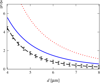
Figure 1: (color online): The detuning $\frac{\delta}{\hbar}$ calculated with $V_{\mathrm{CP}}(x_{1};d)$ (black dashed line) and the corresponding sensitivity (error bars) of a fit to $k=10$ points in time and $m=10$ measurements at each time point. The uncertainty includes the effect of atom-atom interactions and limited resolution of the measurement of population imbalance (see text for details). The input state is the classical spin coherent state. Also, a detuning calculated with $V^{th}_{\mathrm{CP}}(x_{1};d)$ for $T=300$ K (solid blue line) and $T=600$ K (dotted red line) is plotted.

Estimation of the Casimir-Polder force. Since in the presented scheme the information about $\delta$ is acquired by the continuous tunneling of atoms between the wells, the interferometer is suited for measuring forces which decay on a scale of typical inter-well distances of few microns. As an example, we analyze here the measurement of the Casimir-Polder force. We consider an experimentally realistic setup, consisting of a BEC of $N=2500$ ⁸⁷Rb atoms trapped in a double-well potential, with its minima separated by $l=4.8$ $\mu$m and the tunneling energy equal to $E_{J}/\hbar=52.3\ s^{-1}$. When a sapphire plate is placed at a distance $d$ from one of the wells, a Casimir-Polder force acts on the atoms. The exact form of the potential, given by Eq.(26) of Antezza et al. (2004), depends on the dielectric properties of the atoms and the plate, as well as on the temperature $T$ of the latter. If the thermal wavelength $\lambda_{th}=\frac{\hbar c}{k_{B}T}$ of the photons emitted from the plate is much larger than $d$ (as it is for $d\simeq 5\ \mu$m when $T\leq 100$ K), the Casimir-Polder potential is well approximated by $V_{\mathrm{CP}}(x_{1};d)=-\frac{0.24\ \hbar\ c\ \alpha_{0}}{(x_{1}+l/2+d)^{4}}\ \frac{\varepsilon_{0}-1}{\varepsilon_{0}+1}$. Here, $\varepsilon_{0}=9.4$ is the static value of the dielectric function of the sapphire, $c\simeq 3\times 10^{8}\ \frac{\mathrm{m}}{\mathrm{s}}$ is the speed of light and $\alpha_{0}=47.3\times 10^{-30}$ m³ is the static value of ⁸⁷Rb atomic polarizability. The potential shifts the energy minima by $\delta$, calculated as in not (a) using $V(x_{1})=V_{\mathrm{CP}}(x_{1};d)$. If the plate is positioned at $d=4\ \mu$m, then $\delta/\hbar=4.4\ s^{-1}$ and $\frac{\delta}{E_{J}}=0.084$. The period of Rabi oscillations is given by the detuned Rabi frequency and equals 120 ms.

If the temperature of the plate is high, so that the condition $\lambda_{th}\gg d$ is no more satisfied, the Casimir-Polder interactions are described by a temperature-dependent potential $V^{th}_{\mathrm{CP}}(x_{1};d)=-\frac{k_{B}T\ \alpha_{0}}{4\ (x_{1}+l/2+d)^{3}}\ \frac{\varepsilon_{0}-1}{\varepsilon_{0}+1}$. For $T\geq 300$ K, at distance $d$ of few microns, the thermal potential $V^{th}_{\mathrm{CP}}(x_{1};d)$ vastly dominates over the low-temperature one, $V_{\mathrm{CP}}(x_{1};d)$.

In Fig.1, we plot the values of $\delta/\hbar$, as a function of distance $d$, calculated with either $V_{\mathrm{CP}}(x_{1};d)$ (dahsed black line) or $V^{th}_{\mathrm{CP}}(x_{1};d)$ for $T=300$ K (solid blue line) and $T=600$ K (dotted red line). The error bars around the dashed line give the uncertainty $\Delta\delta_{\mathrm{ML}}/\hbar$ of the Rabi interferometer fed by a CSS for a fit to $k=10$ points $t_{i}=\frac{2\pi i}{\omega k}$ in first Rabi period with $m=10$ measurements at each time. In the calculation of the sensitivity, we alse include realistic experimental noise originating from two sources discussed below.

Sources of noise. Spin-polarized fermions are optimal candidates for the implementation of the above interferometric scheme since the s-wave particle-particle interaction is naturally suppressed by the Pauli exclusion principle. In the case of BEC, the atomic interactions can be reduced using the Feshbach resonance method. This technique does not allow for tuning the two body interactions precisely to zero. Some residual interactions always persist and can spoil the sensitivity of the estimation. This can be taken into account by an additional term $E_{C}\hat{J}_{z}^{2}$ in Hamiltonian (1). If the amplitude of the interactions is small, $\gamma\equiv N\frac{E_{C}}{E_{J}}\ll 1$, one can calculate the correction to the evolution operator (2) in first order Dyson expansion with respect to small parameter $\gamma$. Using realistic value $\gamma=0.1$ not (e), the contribution to the error bars in Fig.1 is negligible.

An important source of noise in the Rabi interferometer is given by the limited resolution of population imbalance measurement. This can be taken into account by substituting the ideal probability $p(\{n\}|\delta)$ with the convolution $p_{res}(\{n\}|\delta)=\sum_{n^{\prime}}\mathcal{P}(n,n^{\prime})p(\{n^{\prime}\}|\delta)$, where $\mathcal{P}(n,n^{\prime})$ gives the probability to measure the population imbalance $n^{\prime}$, given the true value $n$. As an example, we take $\mathcal{P}(n,n^{\prime})=\frac{1}{\sqrt{2\pi}\sigma_{\mathrm{res}}}\exp{\big{[}-\frac{(n-n^{\prime})^{2}}{2\sigma_{\mathrm{res}}^{2}}\big{]}}$, with a conservative value $\sigma_{\mathrm{res}}=40$ (the population imbalance is measured with a resolution of $\pm 40$ particles). Then, the ratio $\frac{\Delta\delta_{\mathrm{ML}}}{\delta}$ for the spin coherent state with 2500 atoms increases by a factor of two and this value of $\sigma_{\mathrm{res}}$ is used to present the sensitivity in Fig.1. Even in presence of this noise, the sensitivity is sufficient to precisely distinguish between thermal and zero-temperature regimes of the Casimir-Polder force. This is the main result of this Letter.

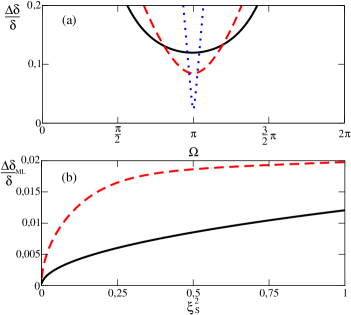
Figure 2: (color online): (a) The relative uncertainty $\frac{\Delta\delta}{\delta}$ as a function of $\Omega$ for $m=1$. Solid black, dashed red and dotted blue lines correspond to $\xi^{2}=$1.0, 0.5, 0.017, respectively. For $\Omega\simeq\pi$, the sensitivities reach optimal point. (b) The relative uncertainty $\frac{\Delta\delta_{\rm ML}}{\delta}$ as a function $\xi^{2}$. The solid black line corresponds to 100 measurements at optimal point. The dashed red line is a result of a fit to $k=$10 different points with $m=$10 repetitions at each point. Here, $N=2500$ and $\frac{\delta}{E_{J}}=0.084$.

Interferometer with squeezed input states. So far, we have discussed the sensitivity of the Rabi interferometer fed with a coherent input state. Below we show that higher sensitivity can be reached when using spin squeezed states. Such states can be created by adiabatically splitting an interacting BEC trapped in a double well potential, as recently experimentally demonstrated in Esteve et al. (2008).

When $N$ is large, and if the input states $|\psi_{inp}\rangle=\sum_{n=0}^{N}c_{n}|n,N-n\rangle$ are symmetrical, i.e. $c_{n}=c_{N-n}$, one can approximate $c_{n}$’s with Gaussians, $c_{n}\propto e^{-(n-\frac{N}{2})^{2}/(4\sigma^{2})}$. Direct calculation gives $\langle\hat{J}_{x}\rangle\simeq\frac{N}{2}e^{-\frac{1}{8\sigma^{2}}}$, $\langle\hat{J}^{2}_{x,y}\rangle\simeq\frac{N^{2}}{8}(1\pm e^{-\frac{1}{2\sigma^{2}}})$ and $\langle\hat{J}^{2}_{z}\rangle\simeq\sigma^{2}$. According to the definition of spin squeezing Wineland et al. (1994), $\xi^{2}=N\frac{\langle\hat{J}_{z}^{2}\rangle}{\langle\hat{J}_{x}\rangle^{2}}\approx 4\frac{\sigma^{2}}{N}e^{\frac{1}{4\sigma^{2}}}$, states with $\sigma<\frac{\sqrt{N}}{2}$ are called squeezed states and the values of $\xi^{2}$ range from 1 for a CSS, to 0 for a Fock state.

In Fig.2(a) we plot the sensitivity from Eq.(3) for a single measurement ($m=1$) in units of $\delta$ for three values of squeezing, as a function of time in the first Rabi period. We use realistic parameters $N=2500$ and $\frac{\delta}{E_{J}}=0.084$ from previous section. Squeezing of the input state clearly improves the precision.

We also observe that the interferometer has an optimal working time equal to $\frac{\pi}{\omega}$. This suggests the following strategy for estimation of $\delta$. Instead of fitting a curve to a set of equally distributed points in time, one should focus the experimental effort around the working point. In Fig.2(b) we compare the sensitivities $\frac{\Delta\delta_{\rm ML}}{\delta}$ as a function of squeezing parameter $\xi^{2}$ for these two estimation strategies. The solid black line is obtained using the optimal strategy while the dashed red line results from a fit to $k=10$ points equally spaced in first Rabi period. Even though the optimal time strategy proves better, the difference is smaller than one order of magnitude. Notice that for both protocols precision of the estimation strongly benefits from squeezing of the input state. For the optimal time strategy with a generic symmetrical input state, this can be shown analytically by expressing the sensitivity in terms of the spin squeezing parameter $\frac{\Delta\delta_{\rm ML}}{\delta}=\xi\frac{\omega}{2\delta\sqrt{N}\sqrt{mk}}$.

By finding minimum of $\Delta\delta_{\mathrm{ML}}$ with respect to $\sigma$, one can also show that for a Fock state the sensitivity reaches Heisenberg limit, i.e. $\Delta\delta_{\rm ML}\propto N^{-1}$. Recently, a squeezed state with $\xi^{2}=0.58$ for $N\simeq 2000$ particles was achieved Esteve et al. (2008). As seen in Fig.2(b), such state would allow for 1.5 times improvement of sensitivity in case of optimal point estimation strategy.

Comparison with other interferometric setups. The possibility to use cold/degenerate atoms for the measurement of forces at small distances has lead to a number of proposals and experiments Carusotto et al. (2005); Sorrentino et al. (2009); Ferrari et al. (2006); Wolf et al. (2007); Pasquini et al. (2004); Harber et al. (2005); ju Lin et al. (2004); Obrecht et al. (2007). In Obrecht et al. (2007), the gradient of the Casimir-Polder force was deduced from the shift of the frequency of the collective oscillations of a BEC in a trap put below a surface. The precision of the experiment was not sufficient to make a distinction between thermal and zero-temperature regimes of the force. On the theoretical side, the References Carusotto et al. (2005); Sorrentino et al. (2009), propose to estimate the strength of the interaction between the atoms and a surface using the frequency shift of Bloch oscillations of a cold fermionic gas in a vertical optical lattice. An important aspect of this proposal is the scaling of the sensitivity $\Delta\delta\sim t^{-1/2}$ with the oscillation time $t$. As argued before, this is not the case of the Rabi interferometer. However, when compared to the Bloch oscillations proposal, our setup has the advantage of the sensitivity scaling with the number of particles in the input state $\Delta\delta\sim N^{-\beta}$. As shown above, this scaling is at the shot noise $\beta=1/2$ for a CSS and can be further increased $1/2<\beta\leq 1$ for entangled atoms.

Conclusions. We have shown that a degenerate either bosonic or fermionic gas in a double-well potential can realize a sensitive device for measuring short-range interactions, such as the Casimir-Polder force. Even the interferometer is fed with a classical spin coherent state with moderate number of atoms, and in the presence of realistic experimental noise, the Casimir-Polder force can be measured with precision sufficient to distinguish between its thermal and zero-temperature regimes. The estimation protocol further benefits from squeezing the input state and measuring the population imbalance at the optimal time.

References

- Cronin et al. (2009) A. Cronin, J. Schmiedmayer, and D. Pritchard, Rev. Mod. Phys. 81, 1051 (2009).
- Pezzé et al. (2005) L. Pezzé, L. A. Collins, A. Smerzi, G. P. Berman, and A. R. Bishop, Phys. Rev. A 72, 043612 (2005).
- Lee (2006) C. Lee, Phys. Rev. Lett. 97, 150402 (2006).
- Huang and Moore (2008) Y. Huang and M. Moore, Phys. Rev. Lett. 100, 250406 (2008).
- Jo et al. (2007) G. Jo, Y. Shin, S. Will, T. A. Pasquini, M. Saba, W. Ketterle, D. E. Pritchard, M. Vengalattore, and M. Prentiss, Phys. Rev. Lett. 98, 030407 (2007).
- Schumm et al. (2005) T. Schumm, S. Hofferberth, L. Andersson, S. Wildermuth, S. Groth, I. Bar-Joseph, J. Schmiedmayer, and P. Krüger, Nat. Phys. 1, 57 (2005).
- Gati et al. (2006) R. Gati, B. Hemmerling, J. Folling, M. Albiez, and M. K. Oberthaler, Phys. Rev. Lett. 96, 130404 (2006).
- Böhi et al. (2009) P. Böhi, M. Riedel, J. Hoffrogge, J. Reichel, T. Hänsch, and P. Treutlein, Nat. Phys. 5, 592 (2009).
- Windpassinger et al. (2008) P. Windpassinger, D. Oblak, P. Petrov, M. Kubasik, M. Saffman, C. Alzar, J. Appel, J. Müller, N. Kjergaard, and E. Polzik, Phys. Rev. Lett. 100, 103601 (2008).
- Antezza et al. (2004) M. Antezza, L. P. Pitaevskii, and S. Stringari, Phys. Rev. A 70, 053619 (2004).
- Pasquini et al. (2004) T. A. Pasquini, Y. Shin, C. Sanner, M. Saba, A. Schirotzek, D. E. Pritchard, and W. Ketterle, Phys. Rev. Lett. 93, 223201 (2004).
- Harber et al. (2005) D. M. Harber, J. M. Obrecht, J. M. McGuirk, and E. A. Cornell, Phys. Rev. A 72, 033610 (2005).
- ju Lin et al. (2004) Y. ju Lin, I. Teper, C. Chin, and V. Vuletic, Phys. Rev. Lett. 92, 050404 (2004).
- Obrecht et al. (2007) J. M. Obrecht, R. J. Wild, M. Antezza, L. P. Pitaevskii, S. Stringari, and E. A. Cornell, Phys. Rev. Lett. 98, 063201 (2007).
- Sukenik et al. (1993) C. I. Sukenik, M. G. Boshier, D. Cho, V. Sandoghdar, and E. A. Hinds, Phys. Rev. Lett. 70, 560 (1993).
- Esteve et al. (2008) J. Esteve, C. Gross, A. Weller, S. Giovanazzi, and M. K. Oberthaler, Nature 455, 1216 (2008).
- not (a) We have , where is the double well potential and the mass of the atoms. The parameter , where is the perturbing potential.
- not (b) , , .
- not (c) For , the equation defining the ML estimator, , corresponds to the least square fit formula, .
- not (d) The Fisher information is defined as .
- Arecchi et al. (1972) F. T. Arecchi, E. Courtens, R. Gilmore, and H. Thomas, Phys. Rev. A 6, 2211 (1972).
- not (e) It corresponds to tuning the scattering length to approximately 0.01 Bohr radius; see M. Fattori et al, Phys. Rev. Lett. 101, 190405 (2008).
- Wineland et al. (1994) D. Wineland, J. Bollinger, W. Itano, and D. Heinzen, Phys. Rev. A 50, 67 (1994).
- Carusotto et al. (2005) I. Carusotto, L. Pitaevskii, S. Stringari, G. Modugno, and M. Inguscio, Phys. Rev. Lett. 95, 093202 (2005).
- Sorrentino et al. (2009) F. Sorrentino, A. Alberti, G. Ferrari, V. V. Ivanov, N. Poli, M. Schioppo, and G. M. Tino, Phys. Rev. A 79, 013409 (2009).
- Ferrari et al. (2006) G. Ferrari, N. Poli, F. Sorrentino, and G. M. Tino, Phys. Rev. Lett. 97, 060402 (2006).
- Wolf et al. (2007) P. Wolf, P. Lemonde, A. Lambrecht, S. Bize, A. Landragin, and A. Clairon, Phys. Rev. A 75, 063608 (2007).