Analysis of Supercontinuum Generation Under General Dispersion Characteristics and Beyond the Slowly Varying Envelope Approximation

Abstract.

The generation of broadband supercontinua (SC) in air-silica microstructured fibers results from a delicate balance of dispersion and nonlinearity. We analyze two models aimed at better understanding SC. In the first one, we characterize linear dispersion in the Fourier domain from the calculated group velocity dispersion (GVD) without using a Taylor approximation for the propagation constant. Results of our numerical simulations are in good agreement with experiments. A novel relevant length scale, namely the length for shock formation, is introduced and its role is discussed. The second part shows similar dynamics for a model that goes beyond the slowly varying approximation for optical pulse propagation.

Alejandro B. Aceves

¹ Department of Mathematics

Southern Methodist University

Dallas TX 75275, USA

Rondald Chen², Yeojin Chung¹, Thomas Hagstrom¹ and Michelle Hummel²

²Department of Mathematics and Statistics

The University of New Mexico

Albuquerque, NM 87131, USA

1. Introduction

Since the experimental demonstration of optical soliton propagation in single mode fibers some 20 plus years ago, the investigation of pulse dynamics in nonlinear optical fibers has evolved due to the introduction of novel structures with complex properties, such as photonic crystal and holey fibers [19]. In essence these are examples of engineered dielectric structures aimed at tailoring dispersive characteristics and enhancing nonlinear behavior. A direct outcome in terms of the pulse dynamics that has brought much attention from several experimental groups [11, 14, 13, 10, 7, 29, 26, 22, 17, 24] is the ability to generate broadband supercontinuum spectra. Scientifically this is a departure from soliton dynamics that requires careful analytical and numerical modeling in parallel with the experiments. From the applications point of view, it has opened possibilities never seen before in areas such as frequency metrology [28] and medical diagnostics [16, 25, 23].

Supercontinuum generation (SCG) can arise from various physical processes such as self- and cross-phase modulation, and amplitude modulation [2]. Due to the complex interplay of linear and nonlinear phenomena in SCG dynamics, the theoretical formulation of the SCG mechanism imposes considerable challenges, in particular if this process happens in bulk media [21]. The major recent theory that explains the SCG for relatively low intensities in confined waveguides rests on the evolution and fission of higher-order solitons near the zero-dispersion wavelength in PCFs [17, 18, 12]. If the input wavelength is close to the zero-dispersion wavelength, then the influence of third-order dispersion is strong, thus a higher-order soliton with number $N$ splits into its constituent solitons with the emission of blueshifted nonsolitonic radiation [30]. Since each soliton and its corresponding radiation has a different central frequency, the width of the generated total spectrum increases with increasing soliton number.

Recent experimental observations of supercontina in soft glass (schott SF6) PCF [22, 24], however, suggest an interesting physical mechanism of SCG that cannot be fully explained by the previously known theories. In these experiments, SCG occurs in a dramatic fashion in the very early states of propagation, in particular at a length scale where solitons start forming. Such a phenomenon can only be explained if, initially, nonlinear effects other than soliton fission dominate the physics. Indeed, the underpinning mechanisms that generate supercontinua as reported in most theoretical and experimental studies are shock generation and its dispersive regularization in combination with multisoliton fission. The shock generation is a well known classical phenomenon in fluids and gas dynamics [31]. It also appears in ultra-short pulse propagation in fibers [1, 3, 32]. For ultrashort pulses, the refractive index depends on the pulse intensity, thus the center of the pulse envelope travels with a different speed than that of the trailing and leading edges of the pulse; this leads to an asymmetric shape of the pulse, which invokes shock formation. However, in optical propagation, dispersion plays an important role, preventing a sharp discontinuity. On the other hand, multisoliton generation resulting from small dispersion effects is a consequence of the integrability of the nonlinear Schrödinger equation (NLSE) [33]. Its eventual fission is the result of perturbations to the NLSE such as third order dispersion. Altogether, a universal feature of nonlinear dispersive wave phenomena is that the long term dynamics results from the delicate balance between linear and nonlinear effects.

To better illustrate this delicate balance we begin by studying a simpler model. Here we do not aim at studying a particular fiber; instead we highlight with a minimal number of linear and nonlinear terms different output scenarios. For this, consider the equation

$$i\partial_{z}A+c_{3}\partial^{2}_{t}A+i\epsilon\partial^{3}_{t}A+|A|^{2}A+ic_{2}\partial_{t}(|A|^{2}A)=0,$$ (1)

where $A$ is the envelope of the pulse, $c_{3},\epsilon$ are respectively coefficients for the second and third linear dispersion terms, and $c_{2}$ is the coefficient of a self-steepening term. We can then characterize the dynamics of pulses under different regimes. In all instances we assume an input pulse $A_{inp}=\sqrt{2}/\cosh(t)$.

(i) $0<\epsilon,c_{2},c_{3}\ll 1$ for which $N\approx\frac{\sqrt{2}}{\sqrt{c_{3}}}$ solitons are created and third order dispersion and self-steepening are viewed as perturbations that split the solitons (Figure 1).

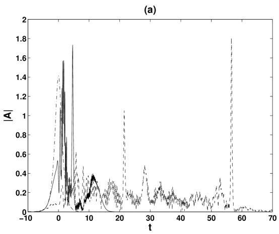
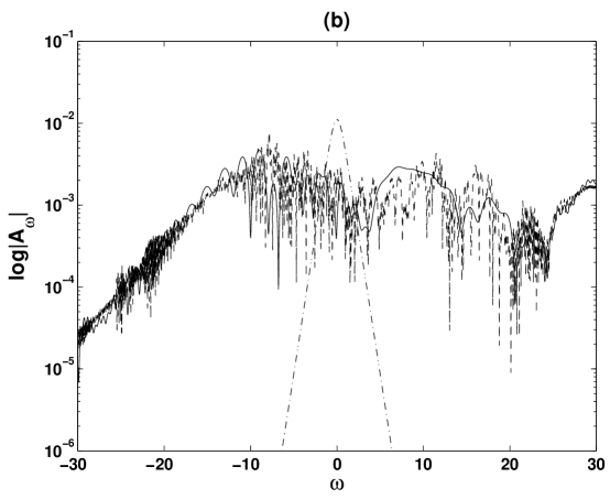
Figure 1. Spectral (bottom) and temporal (top) picture of the pulse profile at $z=0$ (dash-dotted), $z=10$ (solid) and at $z=100$ (dashed). Parameter values $\epsilon=0.01,c_{2}=0.001,c_{3}=0.01$.

(ii) $0<\epsilon,c_{3}\ll 1$ and both much smaller than $c_{2}$, for which the dominant effect is shock formation at a propagation length proportional to $\frac{1}{2c_{2}}$. The dispersion terms are viewed as perturbations which may or may not prevent shock formation. If they do, one expects spectral broadening (Figure 2).

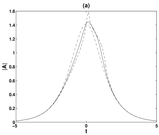
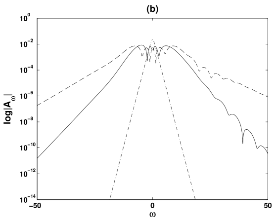
Figure 2. Spectral (bottom) and temporal (top) picture of the pulse profile at $z=0$ (dash-dotted), $z=5$ (solid) and at $z=7$ (dashed). Parameter values $\epsilon=0.0001,c_{2}=0.01,c_{3}=0.0004$.

In contrast, if linear dispersion is dominant and of order one, two cases which illustrate the overall dynamics are, first:

(iii) $c_{3}=1,\ c_{2}\ll\epsilon\ll 1$ for which a soliton emerges and its dynamics under higher order corrections is well described by soliton perturbation theory [8] (Figure 3). In addition, third order dispersion accounts for linear wave resonances which explain the peak in the spectrum (figure 3b).

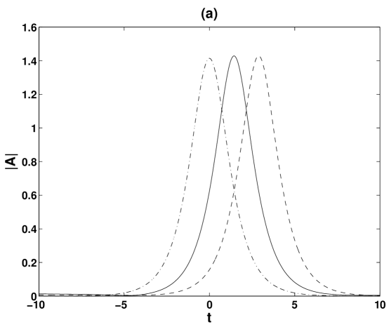
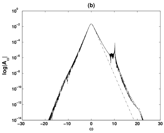
Figure 3. Spectral (bottom) and temporal (top) picture of the pulse profile at $z=0$ (dashed-dotted), $z=10$ (solid) and at $z=20$ (dashed). Parameter values $\epsilon=0.1,c_{2}=0.02,c_{3}=1.0$.

Finally,

(iv) $\epsilon=0.1,\ c_{3}\ll c_{2}\ll 1$ for which there is no soliton (Figure 4).

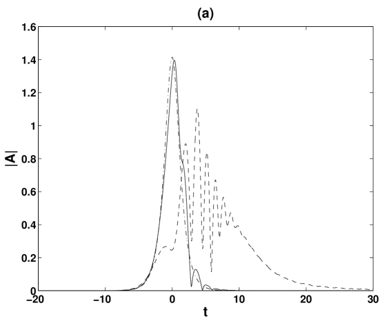
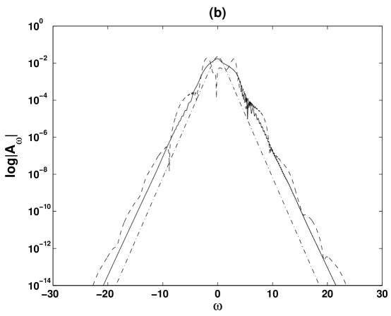
Figure 4. Spectral (bottom) and temporal (top) picture of the pulse profile at $z=0$ (dashed-dotted), $z=1$ (solid), $z=5$ (dashed). Parameter values $\epsilon=0.1,c_{2}=0.01,c_{3}=0.0001$.

Notice the striking difference in the spectrum at the output. While a broadening of the spectrum is achieved in the first two scenarios, this is not the case for the last two, even if, as the temporal profile displayed in case (iv) suggests, the initial pulse is destroyed.

In the next section, we recognize the aformentioned outcomes for a more realistic model describing the pulse dynamics in photonic crystal fibers. The extended model accounts for all competing effects including self-steepening, which we believe is as important as the effect from the fully detailed linear dispersion. As we hoped the first part showed, in order to understand and exploit these phenomena, it is essential to obtain and analyze better these mathematical models. This in addition could explain for each instance in a real experiment what triggered SC generation. To begin with, the accurate broadband modeling of the dispersion relation is required to make sure one does not obtain spurious results, and to do so here we depart from the commonly used approach where a Taylor series expansion of the propagation constant $\beta$ models the dispersive properties in a generalized nonlinear Schrödinger equation (gNLSE). Instead, we develop a mathematical model starting from calculated group velocity dispersion (GVD) curves. Then, we construct the function $\beta(\omega)$ over a broad frequency window and integrate the gNLSE preserving the spectral dependence of the propagation constant. As an illustration, we present our numerical results based on the calculated GVD for an $LP_{01}$ mode in an air-silica microstructured fiber studied by Dudley et al. [13]. Then, similar to what we did with equation (1), we carry out a careful numerical analysis. We find that if the nonlinear self-steepening term is strong enough, the model as it stands produces a shock that is not arrested by dispersion, whereas for weaker nonlinearity the pulse propagates the full extent of the fiber with the generation of a supercontinuum.

Recent studies, in particular for ultrashort pulse dynamics [9], have recognized that the slowly varying envelope approximation may not hold as a good model. In the last part of this paper we discuss how spectral broadening arises without invoking the slowly varying envelope approximation (SVEA).

2. Formulation of the model

The propagation of an electric field wave packet through an optical fiber can be described by gNLSE [1],

$$i\partial_{z}A+{\mathcal{F}}^{-1}[(\beta(\omega)-\beta(\omega_{0}))\hat{A}]+\gamma\left(1+\frac{i}{\omega_{0}}\partial_{t}\right)(A|A|^{2})=0.$$ (2)

Here, the variables $z,T,\omega$ represent propagation distance, time and optical frequency, respectively. The envelope of the wave packet is $A$, and $c,\lambda,\omega_{0},\beta(\omega)$ represent the velocity of light in vacuum, wavelength, central frequency and wave number, respectively. $\mathcal{F}^{-1}$ denotes the inverse Fourier transform, and $\hat{A}$ is the Fourier transform of the pulse envelope. Finally the self-steepening term models the instantaneous nonlinear response function of the medium, which is a good approximation given the temporal lengths of the pulses. The inclusion of a Raman (non-instantaneous) term we believe will only introduce a shift in the peak location in the spectrum (see Fig. 6 and compare with Fig. 5b in [13]).

The effects of fiber dispersion are accounted for by the propagation constant $\beta(\omega)$ which we calculate based on the dispersion profile presented in [13], without performing a Taylor series expansion around the carrier frequency. Using two high-precision numerical integrations of an accurate rational interpolant of the GVD curve, we obtain the GVD function $D(s)$. Then, the group velocity $\nu_{g}(\omega)$ is derived from $D(s)$ through the relation,

$$\frac{1}{\nu_{g}(\omega)}-\frac{1}{\nu_{g}(\omega_{0})}=\int_{\lambda_{0}}^{\lambda}D(s)ds.$$ (3)

By setting $F(\lambda)=\int_{\lambda_{0}}^{\lambda}D(s)ds$, we obtain

$$\nu_{g}(\omega)=\frac{\nu_{g}(\omega_{0})}{1+\nu_{g}(\omega_{0})F(\lambda)}.$$ (4)

Since $\frac{\partial\beta}{\partial\omega}=\frac{1}{\nu_{g}}$, it follows that

$$\frac{\partial\beta}{\partial\omega}=\frac{1}{\nu_{g}(\omega_{0})}+F(\lambda)\sim\frac{1}{c}+F(\lambda).$$ (5)

By integrating Eq. (5) with respect to $\omega$ and using the relation $\lambda=\frac{2\pi c}{\omega}$, we obtain

$$\beta(\omega)-\beta(\omega_{0})=\frac{\omega-\omega_{0}}{\nu_{g}(\omega_{0})}-2\pi c\int_{\lambda_{0}}^{\lambda}\frac{F(\lambda)}{\lambda^{2}}d\lambda.$$ (6)

We employ a frame of reference moving with the pulse at the group velocity $\nu_{g}$ by making the transformation $t=T-z/{\nu_{g}}$. In the end, we obtain

$$i\partial_{z}A-2\pi c{\mathcal{F}}^{-1}\left(\int_{\lambda_{0}}^{\frac{2\pi c}{\omega}}\frac{F(\lambda)}{\lambda^{2}}d\lambda\hat{A}(\omega,z)\right)+\gamma\left(1+\frac{i}{\omega_{0}}\partial_{t}\right)(A|A|^{2})=0.$$ (7)

The resulting equation preserves the complete structure of fiber dispersion which is indeed utilized in experiments. In addition, the equation is valid not only for broad pulses, but also short pulses since the derivation is carried out without the assumption of a pulse centered around a specific carrier frequency (without Taylor series expansion of the propagation constant around a carrier frequency). In the remainder of this section, we present analytical and numerical results obtained from the gNLS (7).

2.1. Optical shock formation

In order to first pay attention to the nonlinear effects governing the mechanism of shock formation [1, 3], we consider the dispersionless case by setting $F(\lambda)=0$ in Eq. (7). In the absence of dispersion, we first split Eq. (7) into an intensity-phase system by adding and subtracting

$${A^{*}}\frac{\partial A}{\partial z} = -\frac{\gamma{A^{*}}}{\omega_{0}}\frac{\partial}{\partial t}(|A|^{2}A)+i\gamma|A|^{4},$$ (8)

$${A}\frac{\partial{A^{*}}}{\partial z} = -\frac{\gamma A}{\omega_{0}}\frac{\partial}{\partial t}(|A|^{2}A^{*})-i\gamma|A|^{4},$$ (9)

where $A^{*}$ is the complex conjugate of $A$.

By defining $I=|A|^{2}$, the addition of Eqs. (8),  (9) gives

$$\frac{\partial I}{\partial z} = -\frac{\gamma}{\omega_{0}}\left[2|A|^{2}\frac{\partial|A|^{2}}{\partial t}+|A|^{2}\left(A^{*}\frac{\partial A}{\partial t}+A\frac{\partial A^{*}}{\partial t}\right)\right]$$ (10)

$$= -\frac{3\gamma}{\omega_{0}}I\frac{\partial I}{\partial t}.$$

The general solution of Eq. (10) is

$$I(z,t)=f\left(t-\frac{3\gamma}{\omega_{0}}Iz\right),$$ (11)

where $f(t)$ is determined by the initial pulse shape, namely, $f(t)=I(0,t)$. The solution form Eq. (11) implies that asymmetric distortion of the pulse will occur eventually.

From Eq. (11), we also find

$$\frac{\partial I}{\partial t}=\frac{f^{\prime}}{1+\frac{3\gamma}{\omega_{0}}f^{\prime}z}.$$ (12)

The resulting equation shows that after a distance $z_{s}=-\frac{\omega_{0}}{3\gamma}\frac{1}{f^{\prime}}$, a singularity in the pulse intensity will be generated, namely, the formation of an optical shock. This shock does play an important role in the spectral broadening once dispersion regularizes it. In other words, the effects of fiber dispersion cannot be ignored. Moreover, the effect of GVD becomes more important as the pulse steepening becomes significant. This phenomenon prevents further steepening of pulse shape, i.e.,an appropriate strength of linear dispersion results in a mechanism that may prevent (or regularize) the shock.

2.2. Numerical solutions of the generalized nonlinear Schrödinger equation

Using the GVD profile employed in experiments [13], we perform our numerical simulations of pulse dynamics based on Eq.  (7). In particular, we consider the propagation of 100$fs$ pulses at 780$nm$ in a 1-m length air-silica microstructured fiber with $\gamma=0.1W^{-1}m^{-1}$. We assume that the input pulse has a form of $A_{0}^{2}/\cosh^{2}\frac{t}{t_{0}}$. As a reference, we find from the previous analysis that the shock length for this input pulse is $z_{s}=22.1cm$ which is much shorter than the actual fiber length, thus in this case shock regularization is a likely scenario for SC generation.

The integration spectrally covers the $400-900nm$ range and, as stated above, it does not require a Taylor expansion of $\beta$. Instead we calculate $\beta$ via two high-precision numerical integrations of the GVD. The numerical evolution is then completed using a standard adaptive ode solver. The results displayed below (figures 5, 6) are in clear qualitative agreement with those in [13]. We should point out two important distinctions between figure 5 in [13] and figure 5 here: we do not capture the peak in the spectrum at wavelengths close to $1200nm$ in 5a,b of [13] and the corresponding pulse (labeled $C$) shown in figure 5c. This is because in our approach we computed the dispersion profile based on the calculated GVD curve shown in figure 2 of [13]. This calculation did not extend to wavelengths beyond $900nm$ and we did not extrapolate such curves. This explains the sharp decay in the spectrum of figure 5 here. Calculations based on a Taylor expansion of $\beta$ which is commonly used, can in principle be extended to any desired spectral range. On the other hand, our result better reproduces the observed supercontinuum spectrum (figure 5a of [13]) in the short (less than $600nm$) wavelength portion and is as good as the Taylor expansion in the intermediate regime.

Finally, figure 5 (right) shows five distinguishable pulses at the output. In figure 6, we spectrally isolate each pulse and find their peaks centered approximately at: $867nm$ (peak 1), $913nm$ (peak 2), $848nm$ (peak 3), $840nm$ (peak 4) $858nm$ (peak 5). As we state below, the spectral separation should be accentuated by the presence of the Raman shift which we did not include in the model. What is most important here is we corroborate spectral broadening and that splitting of pulses occurs, with the spectral shift accounting for differences in soliton velocities.

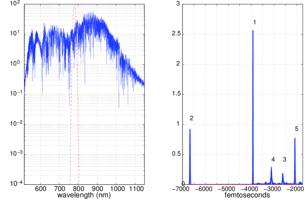
Figure 5. Spectral (left) and temporal (right) picture of the output after $1m$ propagation. All relevant parameters are taken from [5]

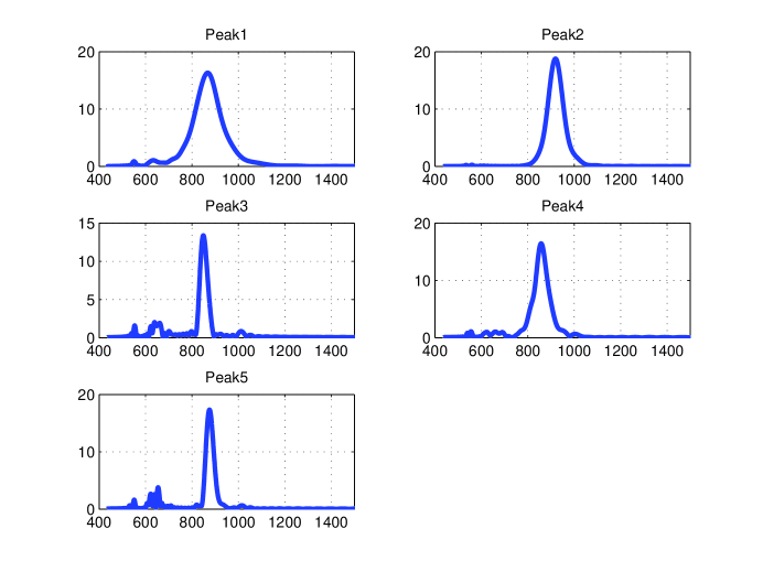
Figure 6. Spectral characteristics of the five distinguishable temporal pulses from figure 5.

In trying to understand the critical balance between linear and nonlinear effects, we now depart from the concrete example to further illustrate this interplay in a series of simulations of the equation shown below, which is no different than equation (7) except that we placed two adjustable constants $c_{2}$($c_{3}$) in front of the self-steepening (linear) term to account for their respective strengths.

$$i\partial_{z}A-c_{3}2\pi c{\mathcal{F}}^{-1}\left(\int_{\lambda_{0}}^{\frac{2\pi c}{\omega}}\frac{F(\lambda)}{\lambda^{2}}d\lambda\hat{A}(\omega,z)\right)+\gamma\left(1+c_{2}\frac{i}{\omega_{0}}\partial_{t}\right)(A|A|^{2})=0.$$ (13)

By proper re-scaling of the propagation variable $z$ and the pulse peak amplitude, one can eliminate the parameter $c_{3}$ but for clarity we analyze our simulations in the 2-parameter space while using the same initial condition. Observe that from (12), an increase of $c_{2}$ effectively means the shock length is reduced. In practice, this shock length reduction can be induced by having shorter input pulses. By allowing ourselves to modulate dispersion and nonlinearity through these two parameters, we hope to highlight how delicate this balance is. Figure 7 which presents a separation between two distinct outcomes was obtained by careful simulations in the $(c_{2},c_{3})$ parameter space. For the region above the curve the shock is not arrested and below the curve dispersion regularizes the shock. It is important to point out the results shown below will strongly depend on the dispersion profile. Nonetheless it is intriguing to see from figure 7 that a universal critical value $(\frac{c_{2}}{c_{3}})_{C}\approx 2.1$ emerges. While one could argue that by modifying $c_{3}$ one departs from a particular photonic structure, what matters is that for every value $c_{3}$ (that is moving vertically in figure 7), this transition always occurs. At this time, we do not have an explanation for it. Furthermore, this property should be tested for different dispersion profiles. To summarize, by performing a series of careful numerical simulations where we look at the relative strengths of the dispersion (measured by a parameter $c_{3}$ that multiplies $F(\lambda)$ in Eq. (1)) and of the self-steepening term (measured by a parameter $c_{2}$) we clearly demonstrate two dynamical regions: one where the singularity due to the shock is not suppressed by dispersion (the region above the curve). In this regime the spectral broadening does not saturate and the numerical solution blows up, clearly suggesting that additional physical mechanisms must be considered. In the second region (the region below the curve) propagation leading to supercontinuum generation or other dynamics similar to those highlighted in the first part of the paper is observed. Although we did not show the curve beyond $c_{3}=0.8$, it should be clear that the point $c_{2}=c_{3}=1$ corresponding to the experimental parameters in [3], is as expected below the curve.

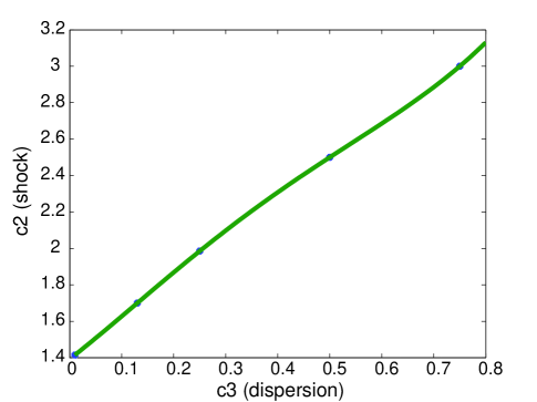
Figure 7. c2 vs c3 curve that separates regions where the numerical simulation blows up (region above the curve) from the region where supercontinuum is numerically observed (region below the curve).

3. SC generation beyond the SVEA

As research into SC generation extends into regimes exhibiting the formation of ultra-short temporal pulses, the validity of the slowly varying envelope approximation (SVEA), even if we incorporate a detailed dispersion profile over a broad spectral range, requires careful consideration. Deriving unidirectional propagation equations for short pulses that would start from Maxwell’s equations and account for dynamics such as higher harmonic generation and sub-cycle shock structure leads to complex envelope equations which can only be solved numerically [20, 15]. One can instead build computational schemes that solve Maxwell’s equations for ultra-short pulses [27]. Careful integration of generalized envelope equations can relove pulses as shot as sub-50 attoseconds [15]. Alternatively, in this section, we illustrate the universality of the features discussed above and observed in many experiments; optical shock formation, dispersion regularization and spectral broadening arise, employing models that do not use the SVEA. Consider the one dimensional nonlinear wave equation derived from Maxwell’s equations,

$$\frac{\partial^{2}A}{\partial z^{2}} = \frac{\partial^{2}A}{\partial t^{2}}+\frac{\partial^{2}}{\partial t^{2}}\int\chi^{(1)}(t-\tau)A(z,\tau)d\tau$$

$$+ \frac{\partial^{2}}{\partial t^{2}}\int\chi^{(3)}(t-\tau_{1},t-\tau_{2},t-\tau_{3})A(z,\tau_{1})A(z,\tau_{2})A(z,\tau_{3})d\tau_{1}d\tau_{2}d\tau_{3},$$

where $\chi^{(1)},\chi^{(3)}$ are linear and nonlinear susceptibilities (for a detailed derivation of this equation, see [9]). Due to the characteristics of its derivation, this equation again preserves the nonlocal nature of the pulse, and thus is valid for both broad and ultrashort pulses. Moreover, it was reported in [9] that $A(t)=\frac{\alpha}{1+(\beta t)^{2}}$ is a stationary solution provided that $\chi^{(3)}=1$ and the Fourier transform of linear susceptibility takes the parabolic form,

$$\hat{\chi}^{(1)}(\omega)=-\frac{1}{8}\frac{\alpha^{2}}{\beta^{2}}(\omega^{2}+3\beta|\omega|+3\beta^{2}),$$ (15)

for some real constants $\alpha$ and $\beta$. While this may not be a realistic dispersion profile, we believe it illustrates well phenomena observed in realistic scenarios.

Here we assume that $\hat{\chi}^{(1)}$ has the form of Eq. (15) with $\alpha=0.2,\beta=0.75$, and an initial pulse of $\frac{0.4}{1+0.75^{2}t^{2}}$. Note that the amplitude of the initial pulse is larger than $\alpha$, and thus the solution will not be stationary and we expect nonlinear effects will be dominant.

We first illustrate the role of nonlinear effects by turning off the linear susceptibility, i.e., ${\chi}^{(1)}=0,$ and setting the nonlinear coefficient $\chi^{(3)}=1$. Numerical simulations of pulse propagation based on Eq. (3) show the output pulse at propagation length $z=5$ and its spectrum (Figure  8). In this case, the nonlinear effects lead to steepening of the pulse shape, which results in the broad spectrum of the output pulse. In the other extreme, Fig.  9 illustrates the pure linear effects by turning off the nonlinearity, i.e., $\chi^{(3)}=0$, and using the linear susceptibility as in (15). At propagation length $z=5$, the pulse has slightly changed its form and also its spectrum. Finally, Fig. 10 presents the combined effects of both nonlinearity and linearity, i.e., $\chi^{(3)}=1$ and $\chi^{(1)}$ as in (15). Compared to Fig. (8), the shock is suppressed by linear dispersion. However, with our choice of input conditions, the nonlinear effect still dominates the dynamics, which induces spectral broadening at finite propagation distances.

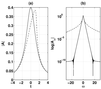
Figure 8. (a) The initial pulse (solid) and output pulse (dashed) after propagation $z=5$, resulted from Eq.(3), where ${\chi}^{(1)}=0$ and $\chi^{(3)}=1$. (b) Spectra of initial pulse (solid) and output pulses (dashed).

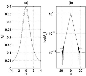
Figure 9. (a) The initial pulse (solid) and output pulse (dashed) after propagation $z=5$, resulted from Eq.(3), where $\chi^{(3)}=0$ and ${\chi}^{(1)}$ as in Eq. (15). (b) Spectra of initial pulse (solid) and output pulse (dashed).

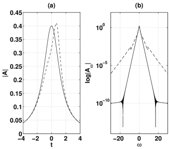
Figure 10. (a) The initial pulse (solid) and output pulse (dashed) after propagation $z=5$ with combining linear and nonlinear effects. The solution is computed based on Eq. (3), where $\chi^{(3)}=1$ and ${\chi}^{(1)}$ as in Eq. (15). (b) Spectra of initial pulse (solid) and output pulse (dashed) presented.

4. Conclusions

Supercontinuum generation is a fascinating and important phenomenon observed in certain nonlinear wave systems. In this work, we first discussed several simple models where we tuned dispersion and nonlinearity so that we could showcase different outcomes. In particular we showed shock driven SC generation as well as soliton-fission driven SC. Next we moved to a model closely related to an existing photonic crystal fiber and showed both SC generation as well as critical shock formation. It is important to emphasize that by properly integrating the dispersive terms for a given photonic microstructured fiber, we capture supercontinuum generation as observed in experiments, likely to greater accuracy than the more common expansion to a finite order of the linear dispersion relation. Our numerical simulations illustrate that for some input conditions, shocks rather than soliton fission appear to be dominant and become the major source of spectral broadening. It is true that soliton fission as seen in many works could be the leading mechanism towards SC generation. Which effect is more dominant and what signatures (if any) of the spectral picture can explain the hierarchy of effects coming into the dynamics remains unclear. Interestingly, two recent theoretical papers using a wave-turbulence approach [4, 6] propose an explanation of SC generation. In [4], the authors claim that coherent structures (solitons, shocks) no longer play a significant role and instead SC results from a nonequilibrium thermodynamic process. This was based in an NLSE-type model which included higher order dispersion, but excluded self-steepening. On the other hand, if self-steepening is included [6], it plays a critical role in thermalization towards a two peak SC spectral profile.An experimental signature of such optical thermalization was recently reported in [5] Overall, as these works clearly illustrate, an accurate mathematical model is essential to better reflect the experimental outcomes. In particular we have a numerical approach at our disposal to study any photonic fiber structure for which GVD profiles have been or can be computed.

Any time one models SC with a slowly varying envelope approximation the question of validity comes to mind. In the last section we presented a simple 1D nonlinear Maxwell’s equation model where spectral broadening is achieved, thus re-enforcing the overall principle that SC generation is universal. While more realistic models that go beyond the SVEA are more difficult to analyze, careful numerical simulations will lead to a better understanding of this very rich phenomenon.

References

- [1] G.P. Agrawal, “Nonlinear Fiber Optics,” 3rd edition, Academic Press, 2001.
- [2] R. Alfano, “The supercontinuum laser source,” New York, Springer-Verlag, 1989.
- [3] D. Anderson and M. Lisak, Nonlinear asymmetric self-phase modulation and self-steepening of pulses in long optical waveguides, Phys. Rev. A, 27 (1983), 1393–1398.
- [4] B. Barviau, B. Kibler, S. Coen and A. Picozzi, Toward a thermodynamic description of supercontinuum generation, Opt. Lett., 33 (2008), 2833–2835.
- [5] B. Barviau, B. Kibler, A. Kudlinski, A. Mussot, G. Millot and A. Picozzi, Experimental signature of optical wave thermalization through supercontinuum generation in photonic crystal fiber Opt. Exp., 17 (2009) 7392–7406.
- [6] B. Barviau, B. Kibler and A. Picozzi, Wave-turbulence approach of supercontinuum generation: Influence of self-steepening and higher order dispersion, Phys. Rev. A, 79 (2009), 063840.
- [7] T. A. Birks, W. J. Wadsworth, and P. S. J. Russell, Supercontinuum generation in tapered fibers, Opt. Lett., 25 (2000), 1415-1417.
- [8] A. Biswas and A. B. Aceves Dynamics of solitons in optical fibres Journ. of Modern Optics 48 (2001) 1135-1150.
- [9] Y. Chung and T. Schäfer, Stabilization of ultra-short pulse in cubic nonlinear media, Phys. Lett. A. 361 (2007), 63–69.
- [10] J. Dudley and S. Coen, Numerical simulations and coherence properties of supercontinuum generation in photonic crystal and tapered optical fibers, IEEE J. Sel. Top. Quantum Electron, 8 (2002), 651–659.
- [11] J. Dudley, G. Genty, and S. Coen, Supercontinuum generation in photonic crystal fiber, Rev. of Mod. Phys., 78 (2006), 1135–1184.
- [12] J. M. Dudley, X. Gu, L. Xu, M. Kimmel, E. Zeek, P. O’Shea, R. Trebino, S. Coen, R. S. Windeler , Cross-correlation frequency resolved optical gating analysis of broadband continuum generation in photonic crystal fiber: simulations and experiments, Opt. Exp., 10 (2002), 1215–1221
- [13] J.M. Dudley, L. Provino, N. Grossard, H. Maillotte, R.S. Windeler, B.J. Eggleton and S. Coen, Supercontinuum generation in air-silica microstructured fibers with nanosecond and femtosecond pulse pumping, JOSA B, 19 (2002), 765–771.
- [14] G. Genty, S. Cohen and J. M. Dudley, Fiber supercontinuum sources (Invited), JOSA B, 24 (2007), 1771–1785.
- [15] G. Genty, P. Kinsler, B. Kibler and J.M. Dudley Nonlinear envelope equation modeling of sub-cycle dynamics and harmonic generation in nonlinear waveguides, Opt. Exp., 15 (2007) 5382–5387.
- [16] I. Hartl, X. D. Li, C. Chudoba, R. K. Ghanta, T. H. Ko, J. G. Fujimoto, J. K. Ranka, and R. S. Windeler, Ultrahigh-resolution optical coherence tomography using continuum generation in an air-silica microstructure optical fiber, Opt. Lett., 26 (2001), 608–610.
- [17] J. Herrmann, U. Griebner, N. Zhavoronkov, A. V. Husakou, D. Nickel, J. C. Knight, W. J. Wadsworth, P. S. J. Russell, and G. Korn, Experimental evidence for supercontinuum generation by fission of higher-order solitons in photonic fibers, Phys. Rev. Lett., 88 (2002), 173901.
- [18] A. V. Husakou and J. Herrmann, Supercontinuum Generation of Higher-Order Solitons by Fission in Photonic Crystal Fibers, Phys. Rev. Lett., 87 (2001), 203901.
- [19] J. C. Knight, T. A. Birks, D. M. Atkin, and P. S. J. Russell, Pure silica single-mode fiber with hexagonal photonic crystal cladding, in Proc. Opt. Fiber Commun. Conf. No. PD3, San Jose, California Feb. (1996).
- [20] M. Kolesik and J. V. Moloney Nonlinear optical pulse propagation simulation: From Maxwell’s to unidirectional equations, Phys. Rev. E, 70 (2004), 036604.
- [21] M. Kolesik, E. M. Wright and J. V. Moloney, Supercontinuum and third-harmonic generation accompanying optical filamentation as first order scattering processes, Opt. Lett., 342 (2007), 2816–2818.
- [22] V. V. R. K. Kumar, A. K. George, W. H. Reeves, J. C. Knight, P. S. J. Russell, F. G. Omenetto, and A. J.Taylor, Extruded soft glass photonic crystal fiber for ultrabroad supercontinuum generation, Opt. Exp., 10 (2002), 1520–1525.
- [23] K. Lindfors, T. Kalkbrenner, P. Stoller, and V. Sandoghdar, Detection and spectroscopy of gold nanoparticles using supercontinuum white light confocal microscopy, Phys. Rev. Lett., 93 (2004), 037401.
- [24] F. G. Omenetto, N. A. Wolchover, M. R. Wehner, M. Ross, A. Efimov, A. J.Taylor, V. V. R. K. Kumar, A. K. George, J. C. Knight, N. Y. Joly, and P. S. J. Russell, Spectrally smooth supercontinuum from 350 nm to 3 m in sub-centimeter lengths of soft-glass photonic crystal fibers, Opt. Exp., 14 (2006), 4928–4934.
- [25] K. Shi, P. Li, S. Yin and Z. Liu, Chromatic confocal microscopy using supercontinuum light, Opt. Exp., 12 (2004), 2096–2101.
- [26] K. Shi, F. G. Omenetto, and Z. Liu, Supercontinuum generation in an imaging fiber taper, Opt. Exp., 14 (2006), 12359–12364.
- [27] J. C. A. Tyrrell, P. Kinsler and G. H. C. New, Pseudospectral spatial-domain: A new method for nonlinear pulse propagation in a few-cycle regime with arbitrary dispersion, Journ of Mod. Opt., 52 (2005), 973–986.
- [28] T. Udem, R. Holzwarth, and T. W. Hänsch, Optical frequency metrology, Nature, 416 (2002), 233–237.
- [29] W. J. Wadsworth, A. Ortigosa-Blanch, J. C. Knight, T. A. Birks, T-P. M. Man, and P. S. J. Russell, Supercontinuum generation in photonic crystal fibers and optical fiber tapers: a novel light source, JOSA B, Special issue on nonlinear optics in photonic crystals and fibres, 19 (2002), 2148–2155.
- [30] P. K. A. Wai, C. R. Menyuk, Y. C. Lee, and H. H. Chen, Nonlinear pulse propagation in the neighborhood of the zero-dispersion wavelength of monomode optical fibers, Opt. Lett., 11 (1986), 464–466.
- [31] G. B. Whitham, “Linear and nonlinear waves,” New York, Wiley Ed., 1974.
- [32] G. Yang and Y. R. Shen, Spectral broadening of ultrashort pulses in a nonlinear medium, Opt. Lett., 9 (1984), 510–512.
- [33] V.E. Zakharov and A.B. Shabat, Exact theory of two dimensional self-focusing and one dimensional self-modulation of waves in nonlinear media, Sov. Physics JETP, 34 (1972), 62–69.