Kinematic constraints on the stellar and dark matter content of spiral and S0 galaxies

Abstract

We present mass models of a sample of 14 spiral and 14 S0 galaxies that constrain their stellar and dark matter content. For each galaxy we derive the stellar mass distribution from near-infrared photometry under the assumptions of axisymmetry and a constant $K_{S}$-band stellar mass-to-light ratio, $(M/L)_{K_{S}}$. To this we add a dark halo assumed to follow a spherically symmetric Navarro, Frenk & White (NFW) profile and a correlation between concentration and dark mass within the virial radius, $M_{\rm DM}$. We solve the Jeans equations for the corresponding potential under the assumption of constant anisotropy in the meridional plane, $\beta_{z}$. By comparing the predicted second velocity moment to observed long-slit stellar kinematics, we determine the three best-fitting parameters of the model: $(M/L)_{K_{S}}$, $M_{\rm DM}$ and $\beta_{z}$. These simple axisymmetric Jeans models are able to accurately reproduce the wide range of observed stellar kinematics, which typically extend to $\approx$ 2–3 $R_{\mathrm{e}}$ or, equivalently, $\approx$ 0.5–1 $R_{25}$. We find a median stellar mass-to-light ratio at $K_{S}$-band of $1.09\,(M/L)_{K_{S},\odot}$ with an rms scatter of 0.31. We present preliminary comparisons between this large sample of dynamically determined stellar mass-to-light ratios and the predictions of stellar population models. The stellar population models predict slightly lower mass-to-light ratios than we measure. The mass models contain a median of 15 per cent dark matter by mass within an effective radius $R_{\mathrm{e}}$ (defined here as the semi-major axis of the ellipse containing half the $K_{S}$-band light), and 49 per cent within the optical radius $R_{25}$. Dark and stellar matter contribute equally to the mass within a sphere of radius $4.1\,\hbox{$R_{\mathrm{e}}$}$ or $1.0\,R_{25}$. There is no evidence of any significant difference in the dark matter content of the spirals and S0s in our sample. Although our sample contains barred galaxies, we argue a posteriori that the assumption of axisymmetry does not significantly affect our results. Models without dark matter are also able to satisfactorily reproduce the observed kinematics in most cases. The improvement when a halo is added is statistically significant, however, and the stellar mass-to-light ratios of mass models with dark haloes match the independent expectations of stellar population models better.

1 Introduction

In the dominant paradigm describing structure formation, initial fluctuations in density are enhanced by gravity until galaxies form in potential wells (White & Rees, 1978; Blumenthal et al., 1984). Numerical simulations and semi-analytic models of galaxy formation are able to reproduce many of the statistical characteristics of galaxies and some of their detailed features (e.g. Kauffmann et al., 1993; Cole et al., 1994; Benson et al., 2003; Baugh, 2006; Somerville et al., 2008). A detailed and consistent theory remains elusive, however, and there are apparent contradictions between the predictions of models and the observations (see, e.g. Baugh, 2006; Mayer et al., 2008, and references therein).

The main stumbling blocks are the significant uncertainties and computational difficulties involved in capturing the baryonic physics that is crucial on sub-Mpc scales. Progress can be made in two ways. Firstly, using observational constraints which are thought to be insensitive to baryonic physics, one can circumvent these uncertainties and directly test the predictions of large-scle structure formation, which is in itself crucially important. Alternatively, one can test formation models with galaxy-scale observations. The outcomes of these tests can be used to refine and improve the models. Perhaps one of the most useful observational constraints for either approach is an understanding of the relative distribution of dark and luminous matter. In this work we aim to measure the radial dark matter distribution in a sample of 28 edge-on disc galaxies. We make cosmologically-motivated assumptions, which allow us to lift certain modelling degeneracies.

It is well-established that, within the optical disc, the kinematics of high surface brightness spiral galaxies can be reproduced by maximal disc models, in which luminous material contributes the maximum amount consistent with the observed rotation curve (e.g. van Albada & Sancisi, 1986; Persic et al., 1996; Palunas & Williams, 2000). The stellar components of maximal disc models typically contribute 75–95 per cent of the rotational velocity at $2.2\,R_{\rm disc}$, where $R_{\rm disc}$ is the scale length of the exponential disc and $2.2\,R_{\rm disc}$ is the radius where the rotational velocity of the exponential disc peaks (Sackett, 1997). This permits dark haloes that comprise 10–45 per cent of the total mass within 2.2 $R_{\rm disc}$. In a Freeman disc (Freeman, 1970), $R_{25}$, the radius of the 25 mag arcsec^-2 isophote occurs at $\approx 3\,R_{\rm disc}$.

Side-stepping the maximal disc assumption, Ratnam & Salucci (2000) demonstrate that rotation curves can be adequately fitted without dark matter. Kassin et al. (2006) avoided the maximal disc assumption entirely by using independent estimates of the stellar mass-to-light ratio inferred from a relationship with colour (Bell & de Jong, 2001; Bell et al., 2003). Most of their models were consistent with a maximal disc. Further evidence is provided by model-independent analysis of rotation curves at intermediate radii (McGaugh et al., 2007).

In the case of elliptical and S0 galaxies, evidence from dynamical modelling and gravitational lensing studies suggests that dark matter makes only a small contribution to the total mass within $R_{\mathrm{e}}$, the radius of the elliptical isophote containing half the light. For example, from the dynamical studies, Gerhard et al. (2001) find that 10–40 per cent of the mass within $R_{\mathrm{e}}$ is dark in their sample of 21 ellipticals, Borriello et al. (2003) find 30 per cent dark matter within $R_{\mathrm{e}}$ by constraining a sample of 221 ellipticals to lie on a fundamental plane, Cappellari et al. (2006) find a median of 30 per cent dark matter within $R_{\mathrm{e}}$ in their sample of 25 ellipticals and S0s, Thomas et al. (2007) find 10–50 per cent dark matter within $R_{\mathrm{e}}$ for a sample of 17 ellipticals and S0s, and Weijmans et al. (2008) find 55 per cent dark matter within 5 $R_{\mathrm{e}}$ in NGC 2974. Lensing studies find similar results. For example, Rusin et al. (2003) find 22 per cent dark matter within 2 $R_{\mathrm{e}}$ of 22 elliptical lenses, Koopmans et al. (2006) find 25 per cent dark matter within the Einstein radius of 15 elliptical lenses (the Einstein radius is approximately equal to the effective radius for galaxy scale lenses), and Bolton et al. (2008) find 38 per cent dark matter inside $R_{\mathrm{e}}$ for 53 elliptical lenses.

However, the total absence of dark matter in ellipticals is sometimes excluded with only low significance due to intrinsic degeneracies in the dynamical models (see, e.g. Romanowsky et al. 2003 and the response by Dekel et al. 2005) and the lack of kinematic tracers at large radii. Moreover, in all cases $\hbox{$R_{\mathrm{e}}$}\ll R_{25}$. The constraints on both the mass of the halo and its extent are therefore less strong for ellipticals than for spirals.

Perhaps the most compelling evidence for the dominance of stellar matter in either ellipticals or high surface brightness disc galaxies comes from the analysis of the bars and spiral arms often present in disc galaxies. These non-axisymmetric features lift the degeneracy between the contributions from luminous and dark matter. This is done by assuming that dark matter is axisymmetric, so all non-circular motions can be attributed to the non-axisymmetric luminous component. This approach has been applied to both bars (e.g. Englmaier & Gerhard, 1999; Weiner et al., 2001) and spiral arms (e.g. Kranz et al., 2003) and provides results consistent with maximal disc studies. Further constraints come from $N$-body simulations of bars, which imply that a significant central dark component would slow or even destroy bars (e.g. Debattista & Sellwood, 2000), while observations systematically indicate that bars are fast (e.g. Aguerri et al., 2003; Gerssen et al., 2003).

To summarize, observational evidence indicates that the kinematics of both spiral and elliptical galaxies can often be reproduced by mass models that include a sub-dominant contribution from dark matter in the optical or central regions. The specific amount required and correlations between halo and luminous galaxy properties are, however, unclear. Note that we have not mentioned low surface brightness and dwarf galaxies, which are dark matter-dominated at all radii (e.g. Persic et al., 1996; de Blok & McGaugh, 1997; Verheijen, 1997; Swaters, 1999) and may provide the most stringent constraints on halo shapes, once observational uncertainties are resolved (e.g. de Blok et al., 2001; Swaters et al., 2003, and references therein). Such galaxies are, however, unrepresentative and extrapolating their results to systems with greater stellar masses may introduce biases. It is therefore crucial to place accurate constraints on the dark matter content of giant, high surface brightness spiral, S0 and elliptical galaxies.

This work uses a modelling technique which is different but qualitatively similar to traditional mass decomposition and rotation curve analyses of spiral galaxies. The key differences are (i) the stellar components of our mass models are based on deep near-infrared photometry, which accurately traces the smooth stellar potential of the galaxy (see Section 2.1), (ii) we lift a degeneracy by making assumptions about the shape of the dark halo that are motivated by the results of cosmological simulations and observational constraints (see Section 2.2) (iii) we lift a further degeneracy (and account for pressure support) by comparing the predicted second velocity moment rather than the rotational velocity to the observed kinematics (see Section 2.3).

We apply this technique to a sample of 28 edge-on spiral and S0 galaxies. We use edge-on galaxies because, under the assumption of axisymmetry, the deprojection is unique. Moreover, when a galaxy is close to edge-on ($i=90^{\circ}$), an inclination error does not propagate on to significant uncertainties in the kinematics in the plane of the galaxy (which is proportional to $\sin i$), and thus on to significant mass uncertainties. The mass models consist of a dark halo component and an unusually detailed parametrization of the projected light. Under justifiable assumptions, the mass model has three free parameters, the stellar mass-to-light ratio, the mass of the dark halo and the velocity anisotropy. We place constraints on these parameters by adjusting them so that the mass model predicts stellar kinematics that closely match those observed. We hope that these simple but powerful quantitative statements will be of use in constraining models of galaxy formation and evolution.

In addition to the halo masses inferred, the constraints we place on the near-infrared stellar mass-to-light ratios are themselves of great interest. There are significant difficulties in modelling the spectral energy distribution of stellar populations in the near-infrared, due to the importance of the complex thermally pulsing asymptotic giant branch at these wavelengths (Maraston, 2005). Moreover, the normalization of the models is uncertain due to a lack of knowledge about the initial mass function of stars. Dynamical measures of the near-infrared stellar mass-to-light ratio like ours, that do not depend on population models and seek to correctly account for dark matter, therefore provide important independent tests of these models.

A final goal of the study is to provide detailed constraints on dark matter in S0 galaxies. The dark matter content of S0s is an important quantity to constrain because the dominant model of S0 formation as faded spirals predicts a simple and verifiable relation between the Tully-Fisher relations of spirals and S0s (e.g. Bedregal et al., 2006, and references therein). Galaxies that lie on a single Tully-Fisher relation linking their luminosities and rotational velocities are believed to have equal dynamical mass-to-light ratios. This will be investigated in more detail in a future paper (Williams, Bureau & Cappellari, in preperation).

This paper is organised as follows: in Section 2 we describe the multi-Gaussian expansion used to model the luminous and dark mass distribution of the galaxies and the dark halo model adopted. We then give an overview of the Jeans modelling technique used to model the stellar kinematics. In Section 3 we present the sample of edge-on galaxies under consideration and describe the photometric and kinematic data. In Section 4 we present the results of our modelling of both the mass distribution and stellar kinematics of the sample, which we discuss in depth in Section 5. Finally, we summarise our conclusions and discuss possibilities for future work in Section 6.

2 Methods

2.1 Modelling the luminous mass distribution

We use multi-Gaussian expansions (MGEs) to create mass models that have a simple analytic form whose kinematics can easily be solved using the Jeans equations. MGE is a method of parametrizing an image of a galaxy as the sum of a finite number of two-dimensional Gaussian functions. The original application of two-dimensional Gaussians to galaxy images (Bendinelli, 1991) was extended to the non-circular case and to more general point spread functions (PSFs) by Monnet et al. (1992) and Emsellem et al. (1994). Here we briefly summarize the method using a formalism due to Cappellari (2002), which we simplify for the special case of axisymmetric edge-on disc galaxies with a luminous component with a constant mass-to-light ratio.

In a coordinate system ($x$, $y$, $z$), where $x$ and $z$ are centred on the galaxy nucleus and point along the major and minor axes in the plane of the sky while the $y$-axis points away from the observer, $\tilde{\Sigma}_{X}(x,z)$ the apparent surface brightness of a galaxy at an arbitrary waveband $X$ can be written as a sum of $N$ two-dimensional Gaussians of apparent width $\tilde{\sigma}_{i}$ in the $x$-direction and $\tilde{\sigma}_{i}\tilde{q}_{i}$ in the $z$-direction:

$$\tilde{\Sigma}_{X}(x,z)=\sum_{i=1}^{N}\frac{L_{i}}{2\pi\tilde{\sigma}^{2}_{i}\tilde{q}_{i}}\exp\left[-\frac{1}{2\tilde{\sigma}^{2}_{i}}\left(x^{2}+\frac{z^{2}}{\tilde{q}^{2}_{i}}\right)\right],$$ (1)

where $L_{i}$ is the total luminosity of the $i$th Gaussian component. We further model the PSF as a circular Gaussian of width $\sigma_{\mathrm{PSF}}$ such that the intrinsic projected light distribution, deconvolved from seeing effects, is

$$\Sigma_{X}(x,z)=\sum_{i=1}^{N}\frac{L_{i}}{2\pi\sigma^{2}_{i}q_{i}}\exp\left[-\frac{1}{2\sigma^{2}_{i}}\left(x^{2}+\frac{z^{2}}{q^{2}_{i}}\right)\right],$$ (2)

where $\sigma_{i}$, the intrinsic width of the $i$th Gaussian in the $x$-direction, and $\sigma_{i}q_{i}$, the intrinsic width in the $z$-direction, are given by

$$\sigma^{2}_{i}=\tilde{\sigma}^{2}_{i}-\sigma^{2}_{\mathrm{PSF}},$$ (3)

$$\sigma^{2}_{i}q^{2}_{i}=\tilde{\sigma}^{2}_{i}\tilde{q}^{2}_{i}-\sigma^{2}_{\mathrm{PSF}}.$$ (4)

Once the projected light distribution is expressed in this simple analytic form, it can be deprojected straightforwardly to give a full three-dimensional model of the light. In this work we deproject by assuming that the galaxy is axisymmetric, but other assumptions about the geometry are possible. Assuming axisymmetry and an edge-on view allows us to trivially transform from the ($x$, $y$, $z$) Cartesian coordinates of the Gaussians on the sky to the ($R$, $\phi$, $z$) cylindrical system of the galaxy, where $R$ is the galactocentric radius, $\phi$ the azimuthal angle and $z$ the axis of symmetry of the galaxy. We also assume a constant stellar mass-to-light ratio $(M/L)_{X}$ to transform the stellar light at waveband $X$ to a stellar mass distribution.

Together these assumptions of axisymmetry, an edge-on view and a constant mass-to-light ratio imply that the intrinsic mass distribution of the luminous component of the galaxy can be written as

$$\rho(R,z)=(M/L)_{X}\sum^{N}_{i=1}a_{i}\exp\left[-\frac{1}{2\sigma_{i}^{2}}\left(R^{2}+\frac{z^{2}}{q^{2}_{i}}\right)\right],$$ (5)

where $a_{i}=L_{i}/(\sqrt{2\pi}\sigma_{i})^{3}q_{i}$.

In this work we determined an optimal MGE parametrization of the images described in Section 3 using the public fitting routine of Cappellari (2002), which minimizes the quantity

$$\chi^{2}_{\mathrm{MGE}}\equiv\sum_{j=1}^{M}\left(\frac{C_{j}(x,z)-\tilde{\Sigma}(x,z)}{C_{j}(x,z)}\right)^{2}$$ (6)

for a given set of $\sigma_{i}$, $q_{i}$ and $L_{i}$, where $M$ is the number of photometric data points $C_{j}$ and $\tilde{\Sigma}$ is the apparent surface brightness of the model.

A MGE is simply a sum of Gaussians reproducing the observed surface brightness. As such, the amplitude of each individual Gaussian, $L_{i}$, is not constrained to be positive as long as the total luminosity and density are positive. Our sample consists of edge-on disc galaxies, which are particularly difficult to fit with solely positive Gaussian terms. As was demonstrated by Bureau et al. (2006), the major axis surface brightness profiles exhibit significant plateaus and secondary maxima. These cannot be fitted by a sum of concentric Gaussians with positive amplitudes, which is necessarily monotonically decreasing with radius. The complex rectilinear or concave two-dimensional structures visible in the isophotes of boxy and peanut-shaped (B/PS) bulges are similarly challenging.

We therefore lifted the positivity constraint on $L_{i}$ when modelling the luminous mass. In doing so, we encountered numerical issues with both the accuracy and stability of the fitting algorithm when using large numbers of Gaussians ($\approx 30$). We solved these by reducing the maximum number of Gaussians in the sum to a relatively small number ($\approx 10$), enabling double precision arithmetic to avoid cancellation errors, and finally, where necessary, tweaking the minimum surface brightness level down to which the fit was constrained by the photometry. We show a typical example of the improvement that is possible when terms with negative amplitude are allowed in Fig. 1. These improved mass models resulted in small but systematic improvements in the accuracy of the modelled kinematics. That a more accurate description of the light gives a more accurate model of the kinematics gives us some confidence that our kinematic modelling methods and assumptions (described in Section 2.3) are not significantly flawed.

The pixel-by-pixel absolute deviation from the photometry of our MGEs is typically 2–4 per cent. For a given constant $(M/L)_{X}$ these small errors are propogated linearly into the mass model. In most previous work, the observed surface brightness distribution of disc galaxies is parametrized using fits to azimuthally averaged radial profiles (e.g. Ratnam & Salucci, 2000; Kassin et al., 2006) or two-dimensional Sersic and/or exponential decompositions (e.g. Gentile et al., 2004). While the terms in our MGEs lack any direct physical association with intrinsic components of the galaxies (bulge, disc, etc.), they reproduce the observed surface photometry more accurately than the simpler parametrizations, and their form is mathematically convenient for Jeans modelling (see Section 2.3).

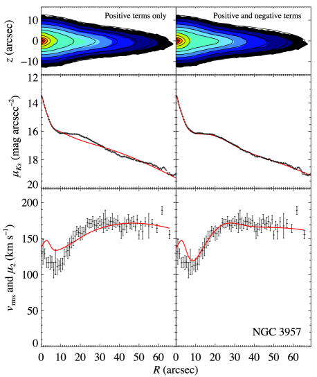
Figure 1: A comparison of the best MGE model with only positive amplitude Gaussians (left-hand panels) and both positive and negative amplitude Gaussians (right-hand panels) for the same object, NGC 3957. The top plots show the $K_{S}$-band surface brightness of the image (filled contours) and model isophotes (solid lines). Contours are separated by 0.5 mag arcsec^-2. The middle plots show the major axis surface brightness profiles of the image (points) and models (solid lines). The bottom panels show $v_{\mathrm{rms}}$ (points), the observed root mean square velocity, and $\mu_{2}$, the best-fitting second moment found by solving the Jeans equations for the MGE model (solid lines). Note that allowing terms in the Gaussian expansion to have a negative amplitude improves both the fit to the photometry and the accuracy with which the kinematics can be reproduced. In order to make the effect clear, the mass model shown here does not include a dark halo.

At large radii, where the model is only weakly constrained by photometric data, models including negative Gaussians can look a little unphysical to the eye (see, e.g., NGC 1886 in Fig. 5). Because there is so little light at these radii, however, we are confident that this does not affect the results significantly. We confirmed this by summing the light of all Gaussians in the MGE models, which can of course be computed analytically, to derive estimates of the total apparent magnitudes of the galaxies. As is shown in Fig. 2, these match the total apparent magnitudes presented in the 2MASS Extended Source Catalog (Jarrett et al., 2000) to within $0.2$ mag. This demonstrates that the excess light sometimes present in the outer regions of MGEs including negative terms is not significant, and that the photometric calibration described in Appendix B is reliable. Fig. 2 also hints that the application of a growth curve method to the relatively shallow 2MASS images of faint objects results in total magnitudes that are systematically too faint (see also Noordermeer & Verheijen, 2007).

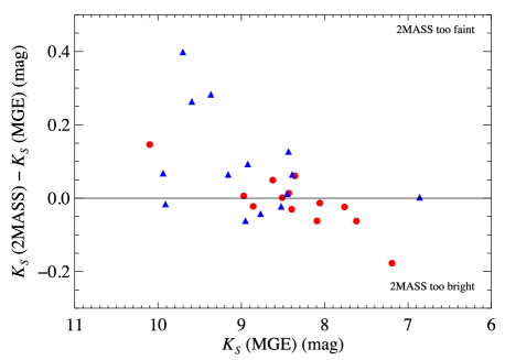
Figure 2: Comparison of the apparent magnitudes of the sample galaxies computed by summing the light of all Gaussians in the best-fitting MGE models with the apparent magnitudes published in the 2MASS Extended Source Catalog. The 2MASS values are derived in the usual way using a growth curve. The methods typically agree to within 0.2 mag. S0s are shown as red circles and spirals as blue triangles.

2.2 Modelling the dark halo mass distribution

If mass models are derived under the assumption that mass follows light then that implicitly assumes that dark matter is not a significant component by mass within the radius probed by the model. Strictly speaking, such models also admit the possibility that the spatial distribution of dark matter closely matches that of the luminous matter, but we know of no physically motivated model of galaxy formation that predicts this behaviour.

We extend our models by explicitly including a dark halo. Although the long-slit kinematic data for each galaxy typically reach $\approx$ 2–3 $R_{\mathrm{e}}$ or, equivalently, $\approx$ 0.5–1 $R_{25}$, they are insufficient to allow a us to constrain the shape of the halo of giant, high surface brightness galaxies like these (see, e.g. Banerjee & Jog, 2008). We therefore emphasise that we are not able to constrain the shapes of the dark haloes. Rather we attempt to probe the more limited question of what fraction by mass of each galaxy is dark assuming the haloes follow the particular one-parameter density profile described below.

Our halo model is motivated by the results of $N$-body simulations of cold dark matter (CDM) in an up-to-date cosmology. In such simulations the dark matter halo density $\rho_{\rm DM}$ is given by the spherically averaged NFW profile:

$$\rho_{\rm DM}(r)=\frac{\rho_{\rm s}}{(r/r_{\rm s})(1+r/r_{\rm s})^{2}}$$ (7)

(e.g. Navarro et al., 1997; Bullock et al., 2001; Wechsler et al., 2002), were $r_{\rm s}$ is a scale radius characterising the location of the ‘break’ in the profile and $\rho_{\rm s}$ is a corresponding inner density.

Rewriting equation (7) in terms of $M_{\rm DM}$, the total dark matter mass enclosed within the virial radius $r_{\mathrm{vir}}$, and defining a concentration parameter $c_{\mathrm{vir}}\equiv r_{\mathrm{vir}}/r_{\rm s}$ implies

$$\rho_{\rm DM}(r)=\frac{M_{\rm DM}}{4\pi A(c_{\rm vir})}\frac{1}{r(r_{\mathrm{s}}+r)^{2}},$$ (8)

where $M_{\rm DM}=4\pi\rho_{\mathrm{s}}r_{\mathrm{s}}^{3}A(c_{\rm vir})$ and

$$A(x)=\ln(1+x)-\frac{x}{1+x}.$$ (9)

The virial radius is defined as the radius within which the mean density is $\Delta\rho_{\mathrm{crit}}$ and $\rho_{\mathrm{crit,0}}=3H_{0}^{2}/8\pi G$ now. Throughout this work we adopt the cosmological parameters found by the Wilkinson Microwave Anisotropy Probe five-year results (WMAP5), i.e. $\Delta=95.1$ and the Hubble constant $H_{0}=100\,h$ km s^-1 Mpc^-1 where $h=0.70$ (Komatsu et al., 2009).

Following Napolitano et al. (2005), we use a key result from simulations of $\Lambda$CDM to eliminate one of the free parameters from equation (8). The simulations demonstrate that concentration and halo mass are correlated: low mass haloes are more concentrated and the concentration–mass relation is well described by a single power law with a slope $\approx-0.1$ (e.g. Navarro et al., 1997; Bullock et al., 2001; Eke et al., 2001; Kuhlen et al., 2005; Neto et al., 2007). We choose the fitting formula presented by Macciò et al. (2008) that is consistent with their WMAP5 simulations over the range $10^{10}\,M_{\odot}<M_{\mathrm{vir}}<10^{15}\,M_{\odot}$:

$$c_{\rm vir}(M_{\rm vir})\approx 9.354\left(\frac{M_{\rm vir}}{h^{-1}10^{12}\,M_{\odot}}\right)^{-0.094},$$ (10)

where $M_{\mathrm{vir}}$ is the total mass enclosed within the virial radius.

We then rewrite this relationship in terms of the dark mass inside the virial radius, rather than the total mass using the equation $M_{\mathrm{vir}}=\alpha\,M_{\mathrm{DM}}$. A number of plausible choices are available to us for the constant $\alpha$: to adopt the cosmological value, to neglect the contribution of baryons entirely, or to adopt some intermediate value. The cosmological value is derived from the ratios of matter density to critical density $\Omega_{\mathrm{m}}=0.258$ and baryon density to critical density $\Omega_{\mathrm{b}}=0.0438$, which together imply

$$\alpha=\frac{\Omega_{\mathrm{m}}}{\Omega_{\mathrm{m}}-\Omega_{\mathrm{b}}}=1.20.$$ (11)

The most extreme ’missing baryon’ scenario, which neglects the contribution of baryons to the total viral mass, implies $\alpha=1$. An intermediate possibility is motivated by the results of observationally constrained halo occupation distribution methods and semi-analytic models, which imply that the stellar mass of a galaxy is typically around 3 per cent of that of its halo, i.e. $\alpha=1.03$. In this work we follow Napolitano et al. (2005) and adopt the cosmological value, $\alpha=1.20$, which gives

$$c_{\mathrm{vir}}(M_{\rm DM})\approx 9.195\left(\frac{M_{\rm DM}}{h^{-1}10^{12}\,M_{\odot}}\right)^{-0.094}.$$ (12)

However, we note that the choice of $\alpha$ makes almost no different to our results. This is because $\alpha$ is immediately raised to the power $-0.094$ in order to define the concentration of the halo; a 20 per cent change in $\alpha$ changes $c_{\mathrm{vir}}$ at the 2 per cent level. If our choice is wrong and results in the introduction of such a small systematic error in $c_{\mathrm{vir}}$, then the consequences for the parameters of the best-fitting mass models are in any case negligible compared to the observational errors.

The dark halo density profile may therefore be written as a function of a single parameter, $M_{\rm DM}$, using equations (8), (9) and (12). We perform a multi-Gaussian expansion of this one-dimensional, single parameter profile to allow us to easily include it in the potential for which we derive model kinematics.

We refrain from including prescriptions for the effects of baryonic contraction on our halo model (e.g. Blumenthal et al., 1986; Gnedin et al., 2004; Abadi et al., 2009). We do this for two reasons. Firstly, our goal is not to determine the detailed shapes of dark haloes but rather the total dark and stellar masses in the optical parts of galaxies. Secondly, while our kinematic data do not allow us to constrain the halo shape, other observational evidence suggests that contracted NFW haloes do not reproduce observed kinematics. (e.g. Gentile et al., 2004; Kassin et al., 2006; Thomas et al., 2007).

2.3 Modelling the stellar kinematics

The most general dynamical methods are particle-based (e.g. de Lorenzi et al., 2007) or orbit-based (e.g. Schwarzschild, 1979; Cappellari, et al., 2007; van den Bosch et al., 2008; Thomas et al., 2009). These powerful methods are so general, however, that a wide range of unrealistic models can be made to fit long-slit data, providing only weak constraints on the parameters of the mass models (see, e.g., fig. 2 of Cappellari & McDermid, 2005). In fact, the stellar kinematics of early-type fast-rotator galaxies are well-described by Jeans models with a cylindrically-aligned velocity ellipsoid with a constant flattening in the $z$-direction (Cappellari, et al., 2007; Thomas et al., 2009). This has lead to the use of a Jeans modelling technique in which such a velocity ellipsoid is assumed. By varying the flattening of the velocity ellipsoid, the Jeans modelling approach has been shown to reproduce a wide range of two-dimensional observed kinematics in the central regions of early-type fast-rotators in the SAURON survey (Cappellari, 2008; Scott et al., 2009) and out to $5\,\hbox{$R_{\mathrm{e}}$}$ in the case of the edge-on S0 NGC 2549 (Weijmans, 2009). The large size of our sample (28 galaxies) allows us to test whether the assumptions provide a good description of our galaxies, but we note that our galaxies are at least as rotationally supported as the SAURON galaxies, so we expect to be even less vulnerable to assumptions about anisotropy.

For convenience we provide an overview of the derivation and solution of the Jeans equations. This is essentially a summary of Sections 2 and 3.1 of Cappellari (2008). Under the assumptions required for the collisionless Boltzmann equation to hold (a smooth potential and steady state), and the further assumption of axisymmetry, the Jeans equations may be written in cylindrical coordinates as

$$\frac{\rho\overline{v_{R}^{2}}-\rho\overline{v_{\phi}^{2}}}{R}+\frac{\partial(\rho\overline{v_{R}^{2}})}{\partial R}+\frac{\partial(\rho\overline{v_{R}v_{z}})}{\partial z} = -\rho\frac{\partial\Phi}{\partial R},$$ (13)

$$\frac{\rho\overline{v_{R}v_{z}}}{R}+\frac{\partial(\rho\overline{v_{z}^{2}})}{\partial z}+\frac{\partial(\rho\overline{v_{R}v_{z}})}{\partial R} = -\rho\frac{\partial\Phi}{\partial z}$$ (14)

(Jeans 1922; Binney & Tremaine 2008). Here $\rho$ is the density, $\Phi$ is the gravitational potential and we use the usual notation

$$\rho\overline{v_{k}v_{j}}\equiv\int v_{k}v_{j}f\;\mathrm{d}^{3}\mathbf{v}.$$ (15)

Even if $\rho$ and $\Phi$ are known (as is the case for our mass models), equations (13) and (14) are still two equations with four unknowns, $\overline{v_{R}^{2}}$, $\overline{v_{z}^{2}}$, $\overline{v_{\phi}^{2}}$ and $\overline{v_{R}v_{z}}$, so they do not specify a unique solution. In order to close the equations one can assume a particular anisotropy, i.e. a relationship between the lengths of the axes of the velocity ellipsoid. We assume here that the velocity ellipsoid is aligned with the cylindrical coordinate system of the galaxy and that the anisotropy in the meridional plane is constant ($\overline{v_{R}^{2}}=b\overline{v_{z}^{2}}$ where $b$ is a constant). Under these assumptions, equations (13) and (14) reduce to:

$$\frac{b\,\rho\overline{v_{z}^{2}}-\rho\overline{v_{\phi}^{2}}}{R}+\frac{\partial(b\,\rho\overline{v_{z}^{2}})}{\partial R} = -\rho\frac{\partial\Phi}{\partial R},$$ (16)

$$\frac{\partial(\rho\overline{v_{z}^{2}})}{\partial z} = -\rho\frac{\partial\Phi}{\partial z}.$$ (17)

These equations are solved for the case of a density and potential described by a sum of Gaussians in Cappellari (2008). Once the observable quantities in the solutions have been projected along the line-of-sight, a single integration gives a model of the second velocity moment, $\mu_{2}$ (see equation [28] of Cappellari 2008). We use the Jeans Anisotropic MGE (jam) routines to perform the calculation.¹ The second velocity moment is compared to the observed root mean square velocity, $v_{\mathrm{rms}}\equiv(v^{2}+\sigma^{2})^{1/2}$, where $v$ is the observed line-of-sight velocity and $\sigma$ the observed line-of-sight velocity dispersion. $v_{\mathrm{rms}}$ is a good approximation to the true second moment. The second moment $\mu_{2}$ is perhaps a less familiar quantity to work with than the circular or line-of-sight velocities, but it has the distinct advantage that it is not necessary to assume a particular ‘splitting’ between ordered and random motions. We discuss its physical meaning in more detail in Section 5.5.3.

The quantity $b$ is often expressed as an anisotropy parameter $\beta_{z}=1-1/b$, where $\beta_{z}=0$ corresponds to isotropy. To give an idea of the kinds of anisotropies observed in real galaxies, Shapiro et al. (2003) found flattened velocity ellipsoids with $0.35\lesssim\beta_{z}\lesssim 0.75$ in the discs of Sa and Sb galaxies. Cappellari, et al. (2007) and Thomas et al. (2009) found more circular ellipsoids for which $\beta_{z}\lesssim 0.4$ in fast-rotator ellipticals and S0s.

If the anisotropy $\beta_{z}$ is free then the predicted kinematics for each galaxy are a function of three parameters: $(M/L)_{X}$, $M_{\rm DM}$ and $\beta_{z}$. We find, however, that for our galaxies, which are rotation dominated, the predicted kinematics along the slit are not very sensitive to the particular choice of $\beta_{z}$. This means that we are unable to place stringent constraints on anisotropy using these data, but it also means that we are not vulnerable to serious systematic errors due to our assumptions about anisotropy.

2.4 Summary of methods and assumptions

To sum up our methods section, we find the stellar component of each mass model by assuming axisymmetry and a constant stellar mass-to-light ratio. To each model we add a dark halo that follows a spherically symmetric NFW profile and assumes the correlation between halo concentration and halo mass defined by equation (12). The total mass model is a function of two parameters, the stellar mass-to-light ratio $(M/L)_{X}$ and the dark halo mass within the virial radius $M_{\rm DM}$. It is expressed as a sum of Gaussians.

The mass model is used to calculate an estimate of the observed stellar kinematics. This is done by solving the Jeans equations under the assumption of constant anisotropy in the meridional plane, yielding the second velocity moment, $\mu_{2}$. This predicted quantity is then compared to the observed root mean square velocity $v_{\mathrm{rms}}\equiv(v^{2}+\sigma^{2})^{1/2}$. The two parameters of the mass model $(M/L)_{X}$ and $M_{\rm DM}$, and the velocity anisotropy $\beta_{z}$ are then adjusted until the predicted stellar kinematics match the observations, placing constraints on those parameters.

Having determined the parameters for each galaxy, we also compute circular the velocities $v_{\mathrm{c}}$ of the stellar, dark and total mass distributions using the numerical techniques described in Cappellari (2002). $v_{\mathrm{c}}$ provides an intuitive measure of the mass enclosed as a function of radius, which is proportional to $v_{\mathrm{c}}^{2}$. The ratio of the squares of the stellar and dark circular velocities is therefore equal to the ratio of the stellar and dark mass enclosed. $v_{\mathrm{c}}$ will also be useful in a forthcoming paper on the Tully-Fisher relation (Williams, Bureau & Cappellari, in preparation).

All mass-to-light ratios in this work are given in solar units, i.e. the mass-to-light ratio at waveband $X$, $(M/L)_{X}$, is in units of $(M/L)_{X,\odot}$.

3 Sample and observations

We apply the methods described above to a sample of 28 edge-on disc galaxies selected by Bureau & Freeman (1999). 14 of the 28 galaxies are classified as S0s and the remaining 14 are Sa–Sb galaxies (see Table 1).

The galaxies in the sample were originally selected to investigate the nature of boxy and peanut-shaped (B/PS) bulges. Of the 28 galaxies, 22 have a B/PS bulge and 6 form a control sample with spheroidal bulges. Galaxies with a B/PS bulges are edge-on disc systems with bulge isophotes above and below the centre of the disc that are either horizontal (boxy) or concave (peanut-shaped). B/PS bulges are thought to simply be bars viewed edge-on. Many $N$-body simulations have shown that bars buckle and thicken soon after formation, resulting in an object that appears peanut-shaped when viewed side-on and boxy when viewed at intermediate angles (e.g. Combes & Sanders, 1981; Combes et al., 1990; Raha et al., 1991; Athanassoula & Misiriotis, 2002). Lütticke et al. (2000) found that 45 per cent of edge-on disc galaxies have a B/PS bulge, which is roughly consistent with the fraction of bars in face-on spirals. Moreover, several studies have identified the kinematic signatures of bars in systems with a B/PS bulge (e.g. Kuijken & Merrifield, 1995; Merrifield & Kuijken, 1999; Bureau & Freeman, 1999; Chung & Bureau, 2004) and a recent study demonstrates the converse by observing kinematic evidence for a B/PS bulge in a face-on barred system (Méndez-Abreu et al., 2008). The sample therefore contains galaxies whose central regions are probably non-axisymmetric. If there is a direct correspondence between B/PS bulges and bars, then the bar fraction in our sample ($\approx 75$ per cent) is representative of that in all disc galaxies ($\approx 65$ per cent, e.g. Sheth et al. 2008). In fact, we will argue in Section 5 the these non-axisymmetries do not affect our results, despite our axisymmetric modelling techniques.

Table 1: Galaxy sample

Galaxy	Type	D	$R_{25}$	$R_{\mathrm{e}}$	$R_{\mathrm{max}}/R_{25}$	$R_{\mathrm{max}}/\hbox{$R_{\mathrm{e}}$}{}$	$K_{S}$	$B$	$M_{K_{S}}$	$M_{B}$
		(Mpc)	(arcsec)	(arcsec)			(mag)	(mag)	(mag)	(mag)
(1)	(2)	(3)	(4)	(5)	(6)	(7)	(8)	(9)	(10)	(11)
B/PS bulges
NGC 128	S0 pec	$59.2$	95.3	18.1	0.49	2.58	8.51	12.46	-25.35	-21.40
ESO 151-G004	S00	$106.9$	42.2	14.1	0.71	2.13	10.29	14.73	-24.85	-20.41
NGC 1381	SA0	$16.8$	76.2	20.1	0.92	3.47	8.36	12.35	-22.76	-18.77
NGC 1596	SA0	$15.3$	116.7	21.7	0.39	2.11	8.06	11.94	-22.86	-18.98
NGC 1886	Sab	$24.5$	96.2	31.1	0.71	2.20	9.16	12.22	-22.79	-19.73
NGC 2310	S0	$15.2$	135.6	39.2	0.64	2.21	8.43	11.48	-22.48	-19.43
ESO 311-G012	S0/a?	$14.5$	122.8	29.7	0.49	2.04	7.76	10.89	-23.05	-19.92
NGC 3203	SA(r)0+	$35.4$	96.6	22.1	0.64	2.80	8.86	12.76	-23.89	-19.99
NGC 3390	Sb	$44.0$	93.8	28.4	0.92	3.03	8.39	11.73	-24.83	-21.49
NGC 4469	SB(s)0/a?	$16.5$	143.3	39.1	0.60	2.21	8.09	12.07	-23.00	-19.02
NGC 4710	SA(r)0+	$16.5$	131.6	44.0	0.73	2.19	7.62	11.69	-23.47	-19.40
PGC 44931	Sbc	$61.2$	91.4	32.3	0.66	1.86	9.60	12.60	-24.34	-21.33
ESO 443-G042	Sb	$35.8$	84.6	35.9	0.86	2.02	9.37	12.56	-23.40	-20.21
NGC 5746	SAB(rs)b?	$30.4$	217.3	51.0	0.67	2.84	6.86	10.11	-25.55	-22.30
IC 4767	S pec	$53.3$	57.8	21.4	0.64	1.72	9.94	13.91	-23.69	-19.72
NGC 6722	Sb	$70.9$	87.9	22.4	0.81	3.19	8.95	12.28	-25.30	-21.97
NGC 6771	SA(r)0+	$64.6$	98.7	15.5	0.52	3.29	8.97	13.24	-25.08	-20.81
ESO 185-G053	SB pec	$66.9$	37.4	12.3	0.77	2.34	9.91	14.04	-24.22	-20.09
IC 4937	Sb	$72.4$	51.5	27.7	0.87	1.63	9.70	13.84	-24.60	-20.46
ESO 597-G036	S00 pec	$123.5$	43.3	18.5	0.87	2.04	10.10	14.76	-25.36	-20.70
IC 5096	Sb	$47.0$	105.7	27.6	0.56	2.14	8.52	12.15	-24.84	-21.21
ESO 240-G011	Sb	$41.4$	167.2	41.5	0.73	2.92	8.43	11.53	-24.65	-21.56
Control sample
NGC 1032	S0/a	$37.0$	106.0	21.0	0.58	2.91	8.40	12.13	-24.44	-20.71
NGC 3957	SA0+	$24.1$	100.7	31.6	0.65	2.08	8.62	12.71	-23.29	-19.20
NGC 4703	Sb	$72.0$	50.9	28.0	1.33	2.43	8.92	13.37	-25.36	-20.92
NGC 5084	S0	$24.2$	297.9	27.0	0.30	3.26	7.19	10.07	-24.73	-21.85
NGC 7123	Sa	$55.3$	80.2	17.1	0.60	2.83	8.45	12.90	-25.26	-20.81
IC 5176	SAB(s)bc?	$24.8$	135.2	29.6	0.46	2.10	8.77	12.02	-23.20	-19.95

Notes. (1) Galaxy name. To ensure continuity with previous studies, the sample is subdivided into B/PS bulges and control galaxies and arranged in order of increasing right ascension. (2) Morphological type taken from Jarvis (1986), de Souza & Dos Anjos (1987), Shaw (1987) and Karachentsev et al. (1993). (3) Distance. The distance of NGC 1381 is taken from Jensen et al. (2003) and that of NGC 1596 from Tonry et al. (2001). NGC 4469 and NGC 4710 are members of the Virgo cluster so we adopt the cluster distance derived by Mei et al. (2007). For all other galaxies we use distances from the NASA/IPAC Extragalactic Database (NED) calculated assuming a WMAP5 cosmology (Komatsu et al. 2009, $H_{0}=70$ km s^-1 Mpc^-1) and a Virgocentic flow model (Mould et al., 2000). (4) Radius of the 25 mag arcsec^-2 $B$-band isophote taken from HYPERLEDA (Paturel et al., 2003). (5) Semi-major axis of the ellipse containing half the light at $K_{S}$-band, measured using the near-infrared photometry presented in Bureau et al. (2006) and the method described in Section 4. (6) and (7) Radius of the last stellar kinematic data point used in this work, expressed as a fraction of $R_{25}$ and $R_{\mathrm{e}}$. (8) Apparent magnitude at $K_{S}$-band derived from the MGE parametrization of the $Kn$-band image (Bureau et al., 2006) calibrated using the 2MASS $K_{S}$-band image (Skrutskie et al., 2006) corrected for Galactic extinction. (9) Apparent magnitude at $B$-band corrected for internal and Galactic extinction taken from HyperLEDA. (10) and (11) Absolute magnitudes derived from the distance and apparent magnitudes in columns (3), (8) and (9).

To parametrize the projected light distribution we use the relatively deep, high-resolution $K$n-band images presented by Bureau et al. (2006). In the course of this work we discovered that the photometric calibration of the images was incorrect (they were too faint by $\approx 0.8$ mag), so we used shallower 2MASS images to recalibrate them, transforming from $K$n to $K_{S}$-band in the process. We describe this procedure in detail in Appendix B. We also correct the 2MASS images and therefore our models for the effects of foreground Galactic extinction using the dust maps of Schlegel et al. (1998). Because the apparent surface brightness distributions that we parametrize are at $K_{S}$-band, the mass-to-light ratios we measure are also at $K_{S}$-band, and therefore denoted $(M/L)_{K_{S}}$. Throughout this work we adopt a value for the absolute magnitude of the Sun at $K_{S}$-band of $M_{K_{S},\odot}=3.29$ (Blanton & Roweis, 2007).

We compare the predicted kinematics of the mass models to major-axis long-slit stellar kinematics presented in Chung & Bureau (2004). We use stellar kinematics rather than gas kinematics because gas is not present and/or not extended in many cases. Where gas is present, it is strongly affected by non-circular motions and shocks in the inner parts of many of the objects (see Bureau & Athanassoula, 1999; Athanassoula & Bureau, 1999). Line-of-sight velocity distributions were extracted using the Fourier Correlation Quotient algorithm (Bender, 1990); the $v$ and $\sigma$ used are those of the best-fitting Gaussian.

4 Results

4.1 Exploring parameter space

Before presenting our best models, we give an overview of how the changes in $(M/L)_{K_{S}}$ and $M_{\rm DM}$ affect the predicted second velocity moment $\mu_{2}$, and what kinds of constraints this allows us to place on these parameters. In general, increasing $(M/L)_{K_{S}}$ shifts the model $\mu_{2}$ to greater velocities at all radii. Increasing $M_{\mathrm{DM}}$ increases $\mu_{2}$ at large radii more than it does at small radii. Fig. 3 demonstrates this behaviour for NGC 1381.

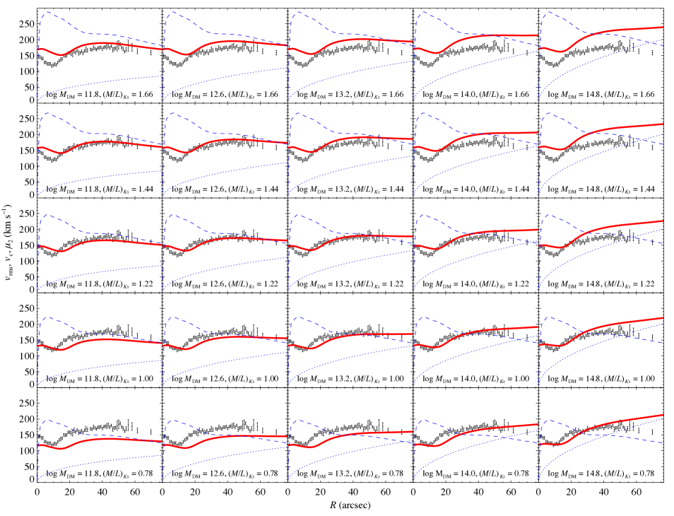
Figure 3: Predicted kinematics for several mass models of NGC 1381, demonstrating the effects of varying the model parameters $M_{\mathrm{DM}}$ and $(M/L)_{K_{S}}$ Each plot shows the observed $v_{\mathrm{rms}}$ (points with error bars) and predicted $\mu_{2}$ (solid red line). We also show the circular velocity of the luminous (dashed blue line) and dark (dotted blue line) components. The text at the bottom of each plot gives the parameters of the mass model in solar units at $K_{S}$-band. The best fitting mass model for this galaxy has $(M/L)_{K_{S}}=1.22$, $M_{\mathrm{DM}}=10^{13.21}$ and $\beta_{z}=0.14$. For this figure we assumed isotropy, i.e. $\beta_{z}=0.0$.

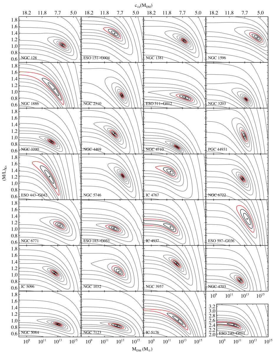
Figure 4: $\chi^{2}$ contour plots for the complete sample showing fit quality as a function of dark halo mass $M_{\rm DM}$ and stellar mass-to-light ratio $(M/L)_{K_{S}}$. The third parameter, the anisotropy $\beta_{z}$, has been marginalized out for this figure, as described in Section 4.1. The red contours are the $3\,\sigma$ confidence levels. The inner black contours are at $1\,\sigma$ and $2\,\sigma$. The cross in each plot shows the location of minimum $\chi^{2}$. The upper horizontal axis shows the halo concentrations $c_{\rm vir}(M_{\rm DM})$ corresponding to $M_{\rm DM}$, as defined by equation (12). With the exception of ESO 240-G011, we arrange galaxies in the same order in which we present them in Table 1. The parameters of the best-fitting model for ESO 240-G011 are outliers, so this galaxy is shown over a different range of $(M/L)_{K_{S}}$.

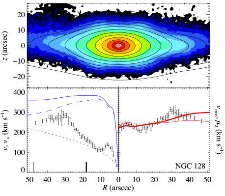
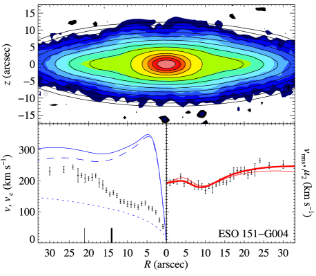
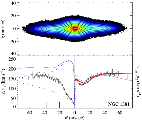
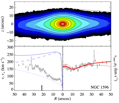
Figure 5: Complete results of the mass and dynamical modelling described in Section 2 for the sample of galaxies with a B/PS bulge. Briefly, the top plot of each panel shows the isophotes of the image (filled contours) and the MGE parametrization of this luminous component (solid black lines). The bottom left plot shows $v$, the observed line-of-sight velocity (points), $v_{\mathrm{c}}$, the total circular velocity (solid blue line), and the circular velocities of the luminous component (dashed blue line) and dark halo (dotted blue line). The thick notch on the $R$-axis shows $R_{\mathrm{e}}$, the $K_{S}$-band effective radius. The thin notch shows $R_{25}/2$, half the $B$-band optical radius. The bottom right plot shows $v_{\mathrm{rms}}$, the observed root mean square line-of-sight velocity (points), $\mu_{2}$, the best-fitting model second velocity moment (thick solid red line) and the best-fitting second moment with no dark halo (thin solid red line). See Section 4.2 for a more detailed explanation of these figures.

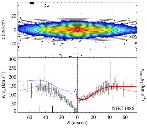
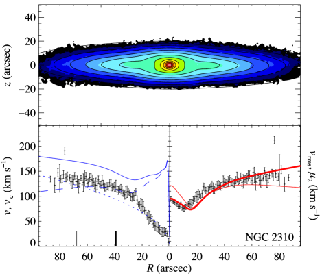
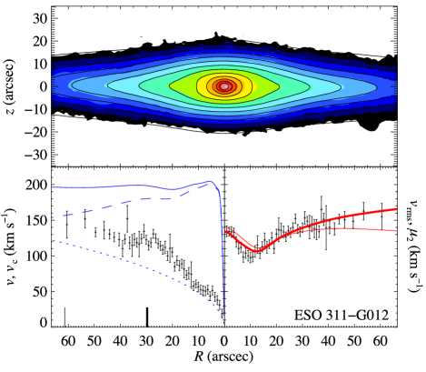
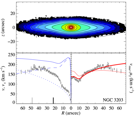
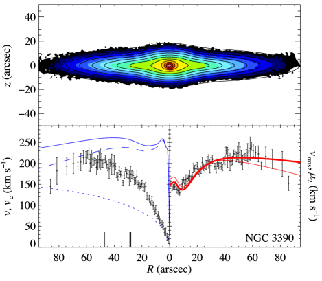
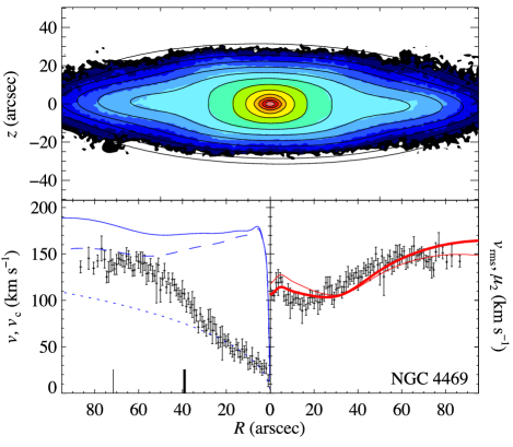
Figure 5: — continued

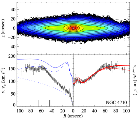
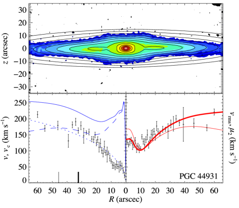
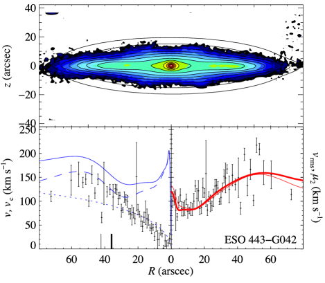
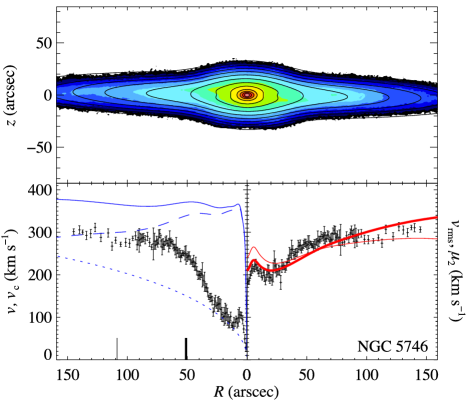
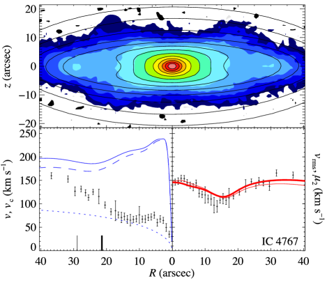
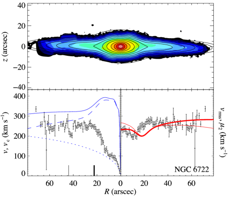
Figure 5: — continued

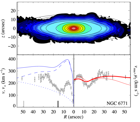
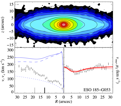
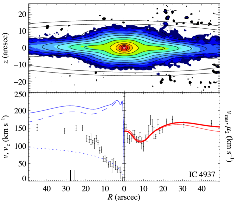
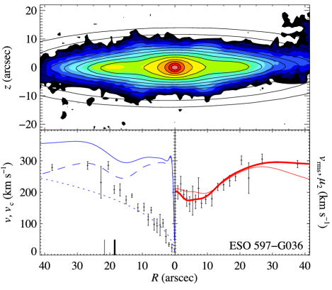
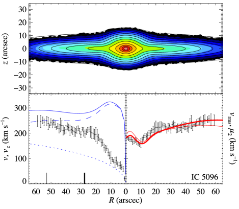
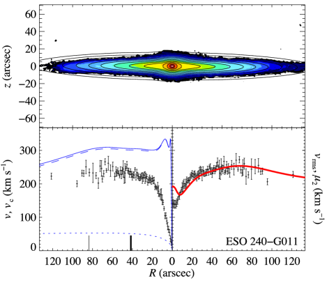
Figure 5: — continued

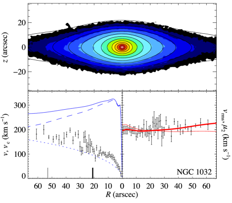
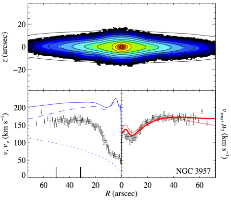
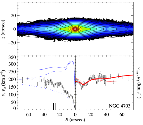
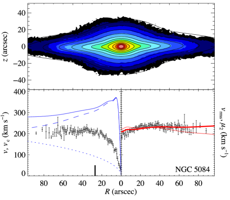
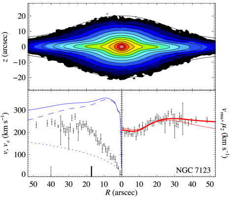
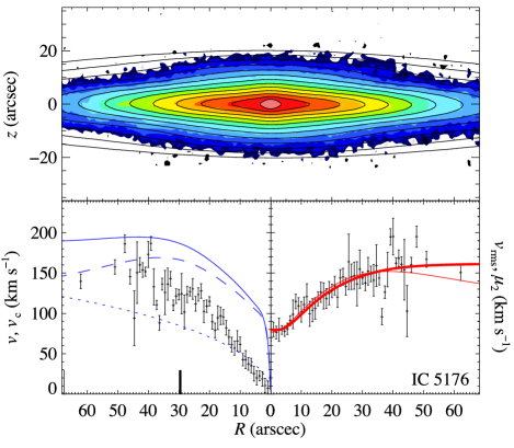
Figure 6: As Fig. 5 but for the control sample.

We define the best-fitting model for each galaxy to be the one with the combination of parameters $(M/L)_{K_{S}}$, $M_{\mathrm{DM}}$ and $\beta_{z}$ that results in a predicted $\mu_{2}$ that most closely matches the observed $v_{\mathrm{rms}}$. The figure of merit, $\chi^{2}$, is therefore defined as

$$\chi^{2}\equiv\sum\frac{\{v_{\mathrm{rms}}-\mu_{2}[M_{\rm DM},(M/L)_{K_{S}},\beta_{z}]\}^{2}}{\Delta v_{\mathrm{rms}}^{2}},$$ (18)

where $\Delta v_{\mathrm{rms}}$ is the error in $v_{\mathrm{rms}}$ and the summation is over all kinematic data points.

We show contour plots of $\chi^{2}$ as a function of these parameters for the complete sample in Fig. 4. For clarity, these plots are marginalized over the anisotropy $\beta_{z}$. This means that the value of $\chi^{2}$ used at each point in $M_{\rm DM}$–$(M/L)_{K_{S}}$ space is set to $\min(\chi^{2}[M_{\rm DM},(M/L)_{K_{S}},\beta_{z}])$ for $0<\beta_{z}<0.75$. The contours become horizontal for $M_{\rm DM}\lesssim 10^{8}M_{\odot}$ because very low mass haloes do not affect the dynamics of the galaxies. There are two classes of $\chi^{2}$ plot: those where we can rule out $M_{\rm DM}=0$ at at least the $3\,\sigma$ confidence level (i.e. where the red contour in Fig. 4 fully encircles the minimum in $\chi^{2}$, e.g. NGC 128 and NGC 1381) and those where we cannot (where the red contour forms an open horizontal ‘tongue’, e.g. NGC 1886 and IC 4937). All galaxies therefore have a best-fitting combination of mass model parameters and allow us to place upper and lower bounds on $(M/L)_{K_{S}}$ and at least an upper limit on $M_{\mathrm{DM}}$. Not all galaxies allow us to place a lower limit on $M_{\mathrm{DM}}$.

4.2 Best-fitting models

The parameters of the best-fitting mass models are shown in Table 2. The MGE parametrizations of the luminous component of each mass model are shown in Table 3. The complete results of the mass modelling and dynamical modelling procedures described in Section 2 are shown in Fig. 5 (B/PS bulges) and Fig. 6 (control sample). In each panel:

1. The top plot shows the image and the luminous component of the mass model. The filled contours are the observed light distribution while the solid lines are the isophotes of the best-fitting MGE model, projected and convolved with the PSF. Contours are separated by 0.5 mag arcsec^-2. The lowest contour is 7 mag arcsec^-2 below the highest. The horizontal axes of these images are registered with those of the kinematic data below, which usually requires that the image be cropped. The full extent of the photometric data is presented in fig. 1 of Bureau et al. (2006).

2. The bottom left plot shows the observed line-of-sight velocity $v$ (points with error bars) and the circular velocities of the total mass model (solid blue line), the luminous component (dashed blue line) and the dark halo (dotted blue line) of the best-fitting mass model (see below). We remind the reader that the ratio of the squares of the dark and luminous circular velocities at a particular radius gives the approximate ratio of dark to luminous matter enclosed within a sphere of that radius (this statement is strictly true for spherical models only).

3. The bottom right plot shows the observed root mean square velocity $v_{\mathrm{rms}}$ (points with error bars), the second velocity moment $\mu_{2}$ of the best-fitting mass model with a dark halo (thick solid red line) and the second velocity moment of the best model without a dark halo (thin solid red line).

We mark the radial axis of the bottom left plot with $R_{25}/2$ and $R_{\mathrm{e}}$, two distance scales used for spiral and elliptical galaxies, respectively. We place a mark at $R_{25}/2$ because $R_{25}$ is always beyond the extent of the stellar kinematic data. Showing both scales aids comparison with previous studies of the influence of dark matter in both classes of galaxies. This is especially interesting because our sample contains many S0s, which represent a transition between spirals and ellipticals.

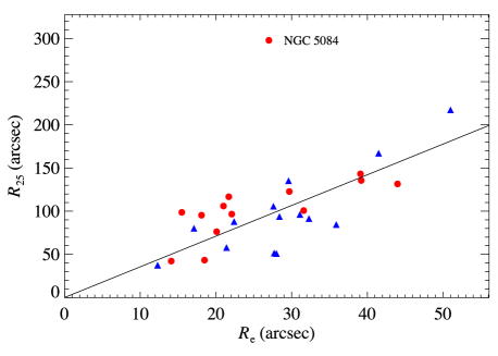
Figure 7: The $B$-band optical radius $R_{25}$ shown as a function of the $K_{S}$-band effective radius $R_{\mathrm{e}}$ (as defined in Section 4.2) for our sample. The line is a linear fit to the data with the intersect constrained to be 0 and the outlier NGC 5084 excluded. The best fit is $R_{25}=3.6\,\hbox{$R_{\mathrm{e}}$}$. Symbols are as in Fig. 2.

We note that the effective radius of very flat objects is particularly sensitive to its definition. We define it here to be the semi-major axis of the ellipse containing half the integrated $K_{S}$-band light, which we determine directly from the photometry. We use the integrated light of the MGE model to determine the half-light radius rather than the more usual growth curve method. Using our MGE models, we tested that this definition yields a value similar to that which would obtained from an ideal observation with the galaxy oriented face-on. We found $R_{\mathrm{e}}$(face-on) $=0.9\hbox{$R_{\mathrm{e}}$}$ (edge-on) $\pm 0.1$. For this definition of $R_{\mathrm{e}}$ and for our sample of edge-on spirals and S0s, $R_{25}\approx 3.6\,\hbox{$R_{\mathrm{e}}$}$ (see Fig. 7). This empirical finding will be used in this paper, and is probably true to within approximately 50 per cent for other edge-on objects, but it should obviously not be applied to less inclined spirals.

An alternative classic definition of $R_{\mathrm{e}}$ is to measure the radius of the circle containing half the light, independent of the apparent ellipticity (Burstein et al., 1987; Roman et al., 1991; Jorgensen et al., 1996). We measured this value for our edge-on galaxies and found that it was typically smaller than the semi-major axis value by a factor $2.0\pm 0.2$. It is therefore rather poorly related to the ‘true’ face-on value and we prefer to integrate within ellipses. It is important, however, to keep our definition of $R_{\mathrm{e}}$ in mind when comparing our results to other studies.

Table 2: Mass and dynamical modelling results

	Best-fitting models with halo				Best-fitting models without halo
Galaxy	$(M/L)_{K_{S}}$	$\log(M_{\mathrm{DM}}/M_{\odot})$	$\beta_{z}$	$\chi_{\mathrm{red}}$	$(M/L)_{K_{S},\mathrm{nohalo}}$	$\beta_{z,\mathrm{nohalo}}$	$\chi_{\mathrm{red,\,nohalo}}$
B/PS bulges
NGC 128	$1.04^{+0.07}_{-0.08}$	$13.61^{+0.45}_{-0.45}$	$0.23^{+0.06}_{-0.06}$	1.86	$1.28^{+0.06}_{-0.06}$	$0.17^{+0.08}_{-0.09}$	2.61
ESO 151-G004	$1.39^{+0.18}_{-0.16}$	$12.31^{+0.77}_{-1.44}$	$0.32^{+0.12}_{-0.20}$	1.16	$1.59^{+0.11}_{-0.11}$	$0.21^{+0.15}_{-0.21}$	1.38
NGC 1381	$1.18^{+0.06}_{-0.08}$	$13.21^{+0.36}_{-0.40}$	$0.14^{+0.05}_{-0.11}$	1.89	$1.48^{+0.04}_{-0.04}$	$0.17^{+0.06}_{-0.08}$	2.85
NGC 1596	$1.26^{+0.16}_{-0.14}$	$14.59^{+0.66}_{-0.99}$	$0.14^{+0.11}_{-0.14}$	1.17	$1.58^{+0.11}_{-0.11}$	$0.12^{+0.11}_{-0.12}$	1.80
NGC 1886	$1.09^{+0.53}_{-0.47}$	$12.53^{+1.22}_{-\ldots}$	$0.43^{+0.26}_{-0.43}$	1.04	$1.57^{+0.16}_{-0.15}$	$0.00^{+0.37}_{-0.00}$	1.12
NGC 2310	$0.88^{+0.09}_{-0.08}$	$13.26^{+0.18}_{-0.27}$	$0.00^{+0.18}_{-0.00}$	1.55	$1.49^{+0.07}_{-0.06}$	$0.00^{+0.03}_{-0.00}$	3.09
ESO 311-G012	$0.82^{+0.10}_{-0.10}$	$13.39^{+0.86}_{-1.17}$	$0.32^{+0.11}_{-0.15}$	1.00	$0.99^{+0.07}_{-0.07}$	$0.24^{+0.12}_{-0.20}$	1.40
NGC 3203	$0.77^{+0.05}_{-0.05}$	$13.17^{+0.18}_{-0.23}$	$0.00^{+0.15}_{-0.00}$	1.92	$1.17^{+0.03}_{-0.03}$	$0.00^{+0.05}_{-0.00}$	3.94
NGC 3390	$0.87^{+0.07}_{-0.08}$	$12.18^{+0.45}_{-0.54}$	$0.00^{+0.09}_{-0.00}$	1.33	$1.06^{+0.04}_{-0.04}$	$0.00^{+0.05}_{-0.00}$	1.63
NGC 4469	$1.12^{+0.11}_{-0.11}$	$12.27^{+0.40}_{-0.59}$	$0.05^{+0.17}_{-0.05}$	1.44	$1.46^{+0.05}_{-0.06}$	$0.00^{+0.09}_{-0.00}$	1.81
NGC 4710	$0.71^{+0.06}_{-0.06}$	$12.31^{+0.31}_{-0.40}$	$0.00^{+0.06}_{-0.00}$	1.08	$0.95^{+0.03}_{-0.02}$	$0.00^{+0.02}_{-0.00}$	1.72
PGC 44931	$1.04^{+0.19}_{-0.16}$	$12.94^{+0.36}_{-0.41}$	$0.00^{+0.17}_{-0.00}$	1.75	$1.66^{+0.13}_{-0.12}$	$0.00^{+0.06}_{-0.00}$	2.79
ESO 443-G042	$1.21^{+0.45}_{-0.57}$	$11.95^{+1.22}_{-2.21}$	$0.47^{+0.28}_{-0.47}$	2.05	$1.68^{+0.19}_{-0.18}$	$0.29^{+0.29}_{-0.29}$	2.10
NGC 5746	$1.23^{+0.07}_{-0.05}$	$13.35^{+0.18}_{-0.22}$	$0.00^{+0.02}_{-0.00}$	2.13	$1.64^{+0.04}_{-0.03}$	$0.00^{+0.00}_{-0.00}$	3.08
IC 4767	$1.36^{+0.18}_{-0.16}$	$11.45^{+0.72}_{-1.89}$	$0.24^{+0.14}_{-0.23}$	1.23	$1.51^{+0.13}_{-0.12}$	$0.17^{+0.17}_{-0.17}$	1.39
NGC 6722	$1.14^{+0.10}_{-0.09}$	$12.72^{+0.27}_{-0.36}$	$0.14^{+0.09}_{-0.14}$	2.22	$1.47^{+0.06}_{-0.06}$	$0.20^{+0.08}_{-0.11}$	2.68
NGC 6771	$1.12^{+0.12}_{-0.12}$	$13.30^{+0.68}_{-0.81}$	$0.29^{+0.11}_{-0.18}$	2.05	$1.31^{+0.10}_{-0.10}$	$0.12^{+0.17}_{-0.12}$	2.34
ESO 185-G053	$1.03^{+0.10}_{-0.10}$	$12.22^{+0.81}_{-1.04}$	$0.34^{+0.09}_{-0.14}$	1.73	$1.15^{+0.08}_{-0.08}$	$0.21^{+0.11}_{-0.18}$	1.93
IC 4937	$1.07^{+0.25}_{-0.19}$	$11.45^{+0.90}_{-\ldots}$	$0.18^{+0.21}_{-0.18}$	1.35	$1.21^{+0.13}_{-0.11}$	$0.08^{+0.28}_{-0.08}$	1.38
ESO 597-G036	$1.31^{+0.41}_{-0.41}$	$13.30^{+0.86}_{-1.35}$	$0.37^{+0.26}_{-0.37}$	0.96	$1.87^{+0.23}_{-0.20}$	$0.00^{+0.40}_{-0.00}$	1.44
IC 5096	$1.06^{+0.10}_{-0.09}$	$12.62^{+0.50}_{-0.59}$	$0.00^{+0.06}_{-0.00}$	1.28	$1.29^{+0.05}_{-0.06}$	$0.00^{+0.05}_{-0.00}$	1.70
ESO 240-G011	$2.41^{+0.14}_{-0.14}$	$10.56^{+0.90}_{-\ldots}$	$0.00^{+0.06}_{-0.00}$	1.76	$2.49^{+0.08}_{-0.08}$	$0.00^{+0.08}_{-0.00}$	1.76
Control sample
NGC 1032	$1.10^{+0.18}_{-0.12}$	$12.85^{+0.63}_{-0.90}$	$0.00^{+0.21}_{-0.00}$	0.98	$1.34^{+0.16}_{-0.11}$	$0.08^{+0.18}_{-0.08}$	1.42
NGC 3957	$1.35^{+0.12}_{-0.12}$	$12.27^{+0.49}_{-0.63}$	$0.00^{+0.21}_{-0.00}$	1.22	$1.65^{+0.07}_{-0.06}$	$0.00^{+0.17}_{-0.00}$	1.63
NGC 4703	$0.83^{+0.10}_{-0.09}$	$12.40^{+0.36}_{-0.49}$	$0.09^{+0.23}_{-0.09}$	1.07	$1.06^{+0.08}_{-0.07}$	$0.12^{+0.21}_{-0.12}$	1.65
NGC 5084	$0.89^{+0.04}_{-0.05}$	$13.03^{+0.49}_{-0.59}$	$0.00^{+0.06}_{-0.00}$	1.18	$1.02^{+0.04}_{-0.03}$	$0.00^{+0.08}_{-0.00}$	1.68
NGC 7123	$0.84^{+0.07}_{-0.08}$	$12.62^{+0.81}_{-1.12}$	$0.09^{+0.15}_{-0.09}$	1.18	$0.95^{+0.05}_{-0.05}$	$0.06^{+0.14}_{-0.06}$	1.43
IC 5176	$1.02^{+0.35}_{-0.29}$	$12.49^{+1.17}_{-\ldots}$	$0.34^{+0.23}_{-0.34}$	1.38	$1.33^{+0.11}_{-0.10}$	$0.06^{+0.29}_{-0.06}$	1.44

Notes. All values are computed assuming the distances in Table 1 and are presented in solar units at $K_{S}$-band, $(M/L)_{K_{S},\odot}$ Errors are the formal fitting errors at the $3\,\sigma$ confidence level and neglect the uncertainties discussed in Section 5.5. If the lower error on halo mass $M_{\rm DM}$ is denoted with ellipsis, e.g. $\log M_{\mathrm{DM}}=12.53^{+1.22}_{-\ldots}$, then for this galaxy there is no lower bound on $M_{\mathrm{DM}}$ because $M_{\mathrm{DM}}=0$ cannot be ruled out at the $3\,\sigma$ level. In such cases the quoted value for $M_{\mathrm{DM}}$ is highly unconstrained up to some upper limit, and should be used with caution. $\chi_{\mathrm{red}}$ and $\chi_{\mathrm{red,\,nohalo}}$ are the reduced $\chi$ for the models with and without dark haloes, i.e. $(\chi^{2}/\mathrm{DOF})^{1/2}$ where $\chi^{2}$ is defined in equation (18) and $\mathrm{DOF}$ is the number of degrees of freedom.

5 Discussion

The form of the observed $v_{\mathrm{rms}}$ as a function of radius is usually a double-humped curve (with the inner hump reaching a smaller speed), but sometimes a monotonically rising curve reaching a plateau toward the edge of the disc (rather like a typical observed rotation curve). For example, the observed second moment rises monotonically in NGC 1886 and IC 5176, is almost constant in NGC 1032 and NGC 5084, falls before rising again in NGC 1381 and NGC 2310, and rises then falls then rises again in NGC 3203 and NGC 6771. The position, height, depth and number of bumps is different for each galaxy. The first thing to note, therefore, is that the models are able to reproduce this whole range of behaviours. This is demonstrated by $\chi_{\mathrm{red}}$, the square root of the reduced $\chi^{2}$ of the best-fitting models (see Table 2). The median $\chi_{\mathrm{red}}$ is 1.35 with an rms scatter of 0.40.

These low figures of merit are neither trivial given the wide range of kinematics observed, nor necessarily expected given the simplicity of the models. Although the MGE technique allows for accurate parametrization of the $K_{S}$-band photometry, the deprojected mass models are axisymmetric descriptions of objects that, in most cases, we have good reason to believe are in fact barred (see Bureau & Freeman, 1999; Chung & Bureau, 2004). Our one-parameter description of the dark halo is model dependent, and our total model contains only three free parameters. Despite this, we are able to accurately reproduce the wide range of observed second velocity moment profiles as far as outermost data point, which is typically at $R_{\mathrm{max}}\approx$ 2–3 $R_{\mathrm{e}}$ or, equivalently, $R_{\mathrm{max}}\approx$ 0.5–1 $R_{25}$ (see Table 1). Because of the lack of freedom that we have to vary the shape of the predicted kinematics, it seems that a great deal of information about the kinematical structure of these early-type disc galaxies is contained in their photometry alone. This result is consistent with that of Cappellari (2008):

Given the extent to which our models reproduce the observed kinematics, we are justified to consider that they correspond in some way to the intrinsic properties of the galaxies. We defer our discussion of the possible systematics introduced by our assumptions to Section 5.5.3.

The following discussion of the model parameters is separated into two parts. In the first, we discuss the properties of the best-fitting mass models that include a dark halo. In the second, we discuss those without. We present the three parameters, $(M/L)_{K_{S}}$, $M_{\mathrm{DM}}$ and $\beta_{z}$, of the models with dark haloes and the two parameters, $(M/L)_{K_{S}}$ and $\beta_{z}$, of the models without in Table 2 and Fig. 8. We precede this discussion by noting than none of them appears to correlate with the absolute magnitude $M_{K_{S}}$, the stellar mass or the Hubble type.

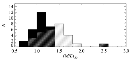
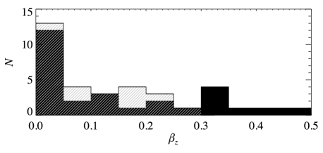
Figure 8: Distributions of the parameters of the best-fitting models with a dark halo (solid black) and without a dark halo (hatched white) in Table 2. We do not show halo masses where there is no lower mass limit. Corresponding values of concentration $c_{\mathrm{vir}}(M_{\rm DM})$ are shown on the upper horizontal axis of the halo mass histogram.

5.1 Models with dark haloes: mass-to-light ratios

We find a median $K_{S}$-band mass-to-light ratio $(M/L)_{K_{S}}=1.09$ with an rms scatter of 0.31. As we noted in the introduction, the mass-to-light ratios are themselves interesting because there are relatively few dynamical measurements of stellar $K$-band mass-to-light ratios and they are important for normalizing and constraining stellar population models in the near-infrared. We therefore compare our values to other available dynamical and stellar population-based measures. Of course there have been many measurements of $(M/L)$ ratio at wavebands other than $K_{S}$ that can be transformed to $K_{S}$ using a global colour. To minimize the uncertainties associated with such transformations, we restrict our discussion to direct determinations at $H$, $K$ or, almost equivalently, $K_{S}$. $K-K_{S}\lesssim 0.03$ mag (the exact value depends on which $K$-band filter is used). For a given stellar mass, this is equivalent to a difference between $(M/L)_{K_{S}}$ and $(M/L)_{K}$ of less than 3 per cent. We neglect this difference in the discussion that follows.

5.1.1 Comparison to previous dynamical measures of stellar $(M/L)_{K}$

Devereux et al. (1987) made among the earliest determinations of near-infrared mass-to-light ratios using nuclear dispersions and 1.65 $\mu$m (i.e. $H$-band) photometry. For 72 bright spiral, S0 and elliptical galaxies, they found a mean $(M/L)_{H}$ = 0.94 (where we have updated the value they adopted for $M_{\odot,H}$ with a more recent determination). For a constant characteristic $H-K_{S}$ color of 0.28 mag (Jarrett et al., 2003), this implies $(M/L)_{K_{S}}\approx 0.7$. Kranz et al. (2003) determined maximal disc $(M/L)_{K}$ ratios by comparing the results of hydrodynamical simulations to the observed spiral patterns in spiral galaxies. For a sample of five high surface brightness late-type spiral galaxies, they find a mean $(M/L)_{K}\approx 0.6$. In the case of the small elliptical galaxy Cen A ($\sigma_{\rm e}\approx 140$ km s^-1), there are two independent dynamical measurements of $(M/L)_{K}$ (Silge et al., 2005; Cappellari et al., 2009), both of which are $\approx 0.7$. We therefore find that our direct dynamical measures of $(M/L)_{K_{S}}$, which we believe accurately account for dark matter, are somewhat larger than most previous dynamical estimates at around the 1–$2\,\sigma$ significance level. Our method depends on an assumed single-parameter NFW dark halo, rather than the two-parameter isothermal halo used by Kranz et al. (2003). It is however somewhat more direct and avoids the maximal disc assumption.

5.1.2 Comparison to previous stellar population measures of $(M/L)_{K}$

If our modelling assumptions are justified, then because mass is correctly shared between the luminous and dark components, the $(M/L)_{K_{S}}$ ratios that we measure should agree with those predicted by well-calibrated stellar population models. A forthcoming paper will present an extensive stellar population analysis of the galaxies in our sample using absorption line strengths and a more complete comparison to the predictions of models. For now though, we perform a preliminary check by comparing our results to the predictions of two models. In Fig. 9 we show the dynamically determined stellar mass-to-light ratios of our sample galaxies as a function their $B-K_{S}$ colour. We also show the predictions of two independent stellar population models.

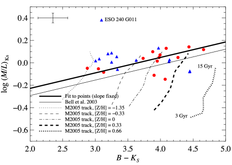
Figure 9: Stellar $(M/L)_{K_{S}}$ against $B-K_{S}$ colour. The data points use the $K_{S}$-band mass-to-light ratios of the stellar components of the best-fitting mass-models including a dark halo, i.e. column (2) of Table 2 and $B$-band magnitudes, corrected for Galactic and internal extinction, are taken from HyperLEDA. $K_{S}$-band magnitudes are derived from our MGE models which incorporate a correction for Galactic extinction. Internal extinction at $K$-band is neglected. A median error bar that does not include the uncertainties introduced by the extinction corrections is shown in the upper left corner (see text). Symbols are as in Fig. 2. The thin straight line is the prediction of the spectrophotometric galaxy evolution models of Bell et al. (2003). The thick straight line is a fit to our data constrained to the slope of the dashed line. The evolutionary tracks for a range of metallicities are from the models of Maraston (2005) and run from 3 Gyr (low mass-to-light ratio) to 15 Gyr (high mass-to-light ratio). Metallicity increases from left to right for these tracks.

We use the $B$-band magnitudes given in HYPERLEDA, which are corrected for both Galactic and internal extinction. We adopt the uncertainties in the uncorrected $B$-band magnitude, which neglect random and systematic errors in the extinction corrections and are therefore lower limits. The Galactic correction is derived from the dust maps of Schlegel et al. (1998). The median Galactic correction at $B$ is 0.2 mag and the uncertainties are probably rather smaller than this. ESO 311-G012 is close to the equatorial plane of the Galaxy (Galactic latitude $b=-8.0^{\circ}$) so the Galactic correction for that galaxy is very large (1.7 mag) and is derived from a region of the Schlegel et al. (1998) maps where extinction corrections are unreliable ($b\lesssim 5^{\circ}$). The $B$-band internal extinction correction is based on the statistical method of Bottinelli et al. (1995), which parametrizes the correction as a function of axial ratio (and therefore inclination) and bulge-to-disc ratio (and therefore morphological type). In exactly edge-on spiral galaxies, the corrections used are both large (0.8–1.5 mag) and somewhat dubious. The $K_{S}$-band magnitudes include a small correction for Galactic extinction (the median correction is 0.02 mag) and neglect internal extinction. The effect on the parameters of the model of neglecting internal extinction in the $K_{S}$-band is discussed in Section 5.5.2, but as far as the $B-K_{S}$ colour is concerned this should introduce a systematic but small error (perhaps 0.1 mag in the spirals and less in the S0s). We therefore conclude that the uncertainties in the $B-K$ colours are dominated by large uncertainties in the corrections to the $B$-band magnitude, especially the internal correction.

The first prediction we compare our results to is the colour–$(M/L)$ relation of Bell et al. (2003). This relation is derived from spectrophotometric galaxy evolution models that use the pegase stellar population model (see Fioc & Rocca-Volmerange 1997 and Bell et al. 2003) with a Salpeter initial mass function (IMF) modified by globally scaling down the stellar mass by a factor of 0.7. Bell et al. (2003) do not present relations involving near-infrared colours, so we adopt a characteristic $R-{K_{S}}$ colour of 2.2 mag to derive the line shown in Fig. 9 from their $(B-R)$–$(M/L)_{K_{S}}$ relation, yielding $\log(M/L)_{K_{S}}=0.138-0.568(B-{K_{S}})$. Bell & de Jong (2001) do use near-infrared colours, but their relations are based on a small selection of ages and metallicities rather than the distribution observed in the local universe. This leads them to derive a rather flatter relation than the ones shown in Bell et al. (2003).

We show in Fig. 9 a further comparison to an independent set of stellar population models from Maraston (2005) that predict $K$-band mass-to-light ratios for stellar populations with ages less than 15 Gyr and metallicities $-1.33<[\mathrm{Z/H}]<0.67$. The models include a semi-empirical treatment of the thermally pulsing asymptotic giant branch, to which the near-infrared luminosity is particularly sensitive. We show models assuming a Kroupa IMF. These tracks can be transformed to predictions for the scaled down Salpeter IMF of Bell et al. (2003) and the normal Salpeter by adding 0.09 dex and 0.24 dex respectively to the logarithm of the $(M/L)$ ratio. In this case we show evolutionary tracks for a range of metallicities rather than a statistical characterisations of local galaxies.

As the figure demonstrates, the predictions of the Bell et al. (2003) galaxy evolution models are below our dynamical determinations in all but four cases. A power law fit to our models, constrained to the same slope as the Bell et al. (2003) line and from which the outlier ESO 240-G11 is excluded, implies a systematic offset of $\Delta\log(M/L)_{K_{S}}=0.06$ dex. At least part of this small offset could be due to the introduction of a systematic error in the approximate transformation of the Bell et al. (2003) to $B-K_{S}$. Our measurements are systematically toward the upper end, if not outside, the range of values predicted by the Maraston (2005) models. If the stellar population models are correct, this implies systematically old stellar populations, $\gtrsim 10$ Gyr. These differences are intriguing and could suggest problems in the stellar evolution models or the IMFs adopted, but we note four reasons which lead us to argue that our findings are broadly consistent with their predictions. Firstly, there is a random scatter of $0.1$– $0.2$ dex in the Bell et al. (2003) relation (larger at the blue end). Secondly, there may be systematic errors in the $(B-K_{S})$ colours adopted for our sample of edge-on galaxies due to internal extinction. These are difficult to quantify. Thirdly, in the case of the Maraston (2005) tracks, the mass-to-light ratios are for single stellar population models, while many galaxies, especially spirals, are likely to have composite stellar populations. Finally, our sample of 28 bright early-type disc galaxies is not necessarily representative of local galaxies. We will perform a more detailed comparison on the models and data in a future work.

We end this discussion of the $(M/L)_{K_{S}}$ ratios measured by noting the existence of a significant outlier galaxy, ESO 240-G011, which has $(M/L)_{K_{S}}=2.41\pm 0.14$. This is more than four standard deviations above the median $(M/L)_{K_{S}}$ of the sample. ESO 240G11 has the latest Hubble type in the sample, and later galaxies are generally thought to be more dark matter-dominated. However, our modelling method aims to correctly account for dark matter so $(M/L)_{K_{S}}$ should be the mass-to-light ratio of the stellar component, not the total matter distribution. This particular galaxy therefore remains puzzling.

5.2 Models with dark haloes: dark halo masses

For those galaxies with constrained halo masses, we find a median $M_{\mathrm{DM}}=10^{12.85}\,M_{\odot}$ with an rms scatter of 0.7 dex. Using the concentration–halo mass correlation of Macciò et al. (2008), which our haloes are constrained to lie on, this corresponds to $c_{\rm vir}=7.9$ with an rms scatter of 1.2. These results should be treated with caution, however, because most of the dark mass lies beyond radii at which our models are constrained by either photometry or kinematics. $M_{\rm DM}$ is therefore strongly dependent on the assumptions described in Section 2.2.

With this strong caveat in mind, we note, however, that the virial masses $M_{\rm vir}=1.2\,M_{\rm DM}$ of the models are at least consistent with the predictions of semi-analytic and halo occupation distribution models with respect to their stellar mass. We present a comparison in Fig. 10. Croton et al. (2006) and Somerville et al. (2008) use semi-analytic models of galaxy formation that, among other things, attempt to predict the relationship between the stellar mass and dark halo mass of a galaxy by modelling relevant physical processes such as the growth of structure, cooling, star formation and feedback. Wang et al. (2006) and Moster et al. (2009) use a halo occupation distribution approach to populate a halo catalogue with stellar mass. The halo catalogue is taken from Springel et al. (2005). It is populated to reproduce the local observed stellar mass function and clustering function.

Our models do not agree with the predictions in a few cases, but there is no evidence of any systematic offset. The stellar and virial masses of our mass models do not seem to be correlated. This is not true of the predictions, especially below $M_{\mathrm{vir}}=10^{12}\,M_{\odot}$, which we unfortunately do not probe. The comparison is therefore limited by both a lack of mass range in our sample, and the significant uncertainties in our halo mass determinations. We can only conclude that our galaxies have stellar mass to halo mass ratios consistent with the range predicted by the theoretical models for these halo masses. However, the assumptions and observational constraints used to make their predictions are quite independent from ours, so even this relatively weak statement is not trivial. Ignoring the predictions, we note that the spiral galaxies in our sample all have large $M_{*}/M_{\mathrm{vir}}$ ratios relative to the average S0.

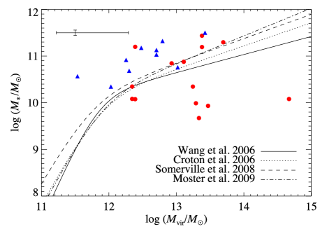
Figure 10: Comparison of the stellar and halo masses of our mass models (data points) to the independent predictions of Wang et al. (2006), Croton et al. (2006), Somerville et al. (2008) and Moster et al. (2009). Median error bars are shown in black in the upper left corner. Symbols are as in Fig. 2.

The dark matter enclosed within a sphere of radius $r$ is given by

$$M_{\rm DM}(r)=M_{\mathrm{DM}}\frac{A(r/r_{\mathrm{s}})}{A(c_{\mathrm{vir}})}.$$ (19)

From this and the ratios of the circular velocities of the dark and stellar components, we can calculate the dark-to-total mass fraction $X_{\mathrm{DM}}$ as a function of radius. We find a mean $X_{\rm DM}(\hbox{$R_{\mathrm{e}}$}{})$ of 15 per cent (10 per cent rms scatter) and a mean $X_{\rm DM}(R_{25})$ of 49 per cent (15 per cent scatter). As we mentioned in the introduction, a maximal disc is strictly defined as one in which the stellar component contributes 75–95 per cent of the rotational velocity at $2.2\,R_{\mathrm{disc}}$, i.e. $X_{\mathrm{DM}}(2.2\,R_{\mathrm{disc}})\leq 45$ per cent (Sackett, 1997) (2.2 $R_{\mathrm{disc}}$ is the radius at which the rotation curve of a thin disc reaches its maximum). The disc scale length of edge-on, barred systems are uncertain (Bureau et al., 2006), but our estimates of $R_{\mathrm{disc}}$ suggest that $X_{\rm DM}(2.2\,R_{\mathrm{disc}})$ is 27 per cent (11 per cent scatter). The best fitting mass model is sub-maximal in only two cases [NGC 2310, $X_{\mathrm{DM}}(2.2\,R_{\mathrm{disc}})=46$ per cent and PGC 44931, $X_{\mathrm{DM}}(2.2\,R_{\mathrm{disc}})=50$ per cent].

We can also determine the radius at which dark and stellar matter contribute equally to the circular velocity and mass enclosed within a sphere. We do this in units of $R_{\mathrm{e}}$ and $R_{25}$ and find $R(X_{\rm DM}=0.5)/\hbox{$R_{\mathrm{e}}$}{}=4.1$ (with rms scatter of 1.3) and $R(X_{\rm DM}=0.5)/R_{25}=1.0$ (with rms scatter of 0.5). These results should be treated with a little caution, however, because in several cases $R(X_{\rm DM}=0.5)>R_{\rm max}$, the last kinematic data point. Beyond the kinematics, the models are obviously particularly model dependent.

As discussed in Section 5.5.1, $X_{\mathrm{DM}}$ and $R(X_{\mathrm{DM}}=0.5)$ are almost unaffected by distance or photometric calibration errors. Finally, we note that there is no evidence of any significant difference between the dark matter content of the spirals and S0s in our sample, at least at the radii within which the models are constrained by the kinematic data.

5.3 Models with dark haloes: anisotropies

The best-fitting anisotropies for our models are in the range $0.0\lesssim\beta_{z}\lesssim 0.5$. As we discussed in Section 2.3, however, the constraints on these measurements are weak because the galaxies in our sample are rotation-dominated and we do not have integral field data. Moreover, we assume a constant anisotropy throughout the galaxy, which is of course a significant simplification, since many of our galaxies have a bulge, bar and disc. With these caveats in mind, the typical anisotropy we find is broadly consistent with the average of previous observations of ellipticals, that are expected to have similar dynamics to the bulges ($\beta_{z}\lesssim 0.4$, Cappellari, et al. 2007; Thomas et al. 2009) and discs ($0.35\lesssim\beta_{z}\lesssim 0.75$, Shapiro et al. 2003).

5.4 Neglecting dark matter

As discussed in the introduction, previous studies have shown that it is usually possible to construct mass models of bright spiral galaxies that reproduce the general form of their rotation curves within $R_{25}$ with no or only a sub-dominant contribution from dark matter. It is therefore not surprising that, in some cases, the improvement in fit quality when a dark halo added is not overwhelming.

How many galaxies can we fit without a dark halo? Many of the second velocity moments of the best mass models without a dark halo are, by eye at least, satisfactory fits to the observed kinematics (compare the thin red lines to the data points in the lower right plot of each panel in Figures 5 and 6). In the formal sense, in four cases (NGC 1886, IC 4937, ESO 240-G011, and IC 5176) the removal of the dark halo does not improve the fit at the $3\,\sigma$ level.

We therefore now discuss an Occam’s Razor argument which states that, since we can fit some of these galaxies well without dark matter, dark matter is not a significant component by mass within the radii probed by our kinematic data (0.5–1 $R_{25}$ or 2–3 $R_{\mathrm{e}}$) in at least those cases. We reject this argument because the parameters of our best fitting mass models with dark matter are in line with independent expectations, whereas those for the haloless models are not. For example, the mass-to-light ratios we measure for mass models without haloes are inconsistent with stellar population results. We find the median $(M/L)_{K_{S},\,\mathrm{nohalo}}=1.25(M/L)_{K_{S}}$, where $(M/L)_{K_{S},\,\mathrm{nohalo}}$ is the stellar mass to light ratio measured using a mass model without a dark halo. The $(M/L)_{K_{S},\,\rm nohalo}$ we measure is therefore significantly higher than the predictions the stellar population models of Bell et al. (2003) and Maraston (2005). Either the stellar population models and their assumptions are flawed, or the stellar mass models without dark matter have too much mass. The halo sizes (and concentrations) of the models with dark matter also match the expectations of galaxy formation. Of course, adding another free parameter to a model is always going to improve the quality of the fit, but if the true halo of a galaxy is not significant (or not present), the agreement between the halo masses that most improves the fits and the predictions and the expectations of $\Lambda$CDM would be a striking coincidence.

Indeed, the fact that the $(M/L)$ ratio of a mass model including only stars systematically exceeds that of a mass model accounting for dark matter or a stellar population estimate can be used to estimate how ‘wrong’ the former is. The median $(M/L)_{K_{S},{\rm nohalo}}$ must be decreased by 20 percent [$\Delta\log(M/L)\approx-0.10$] to match $(M/L)_{K_{S}}$, the dynamically determined stellar mass-to-light ratio with dark matter. This is similar to the finding of Cappellari et al. (2006), that the median $I$-band dynamical $(M/L)$ ratio neglecting dark matter must be decreased by 30 per cent [$\Delta\log(M/L)_{I}\approx-0.15$] to match the stellar population $(M/L)$ ratio.

5.5 Uncertainties and assumptions

5.5.1 Random errors

The errors presented in Table 2 are $3\,\sigma$ formal fitting errors. These neglect random errors due to distance uncertainties and photometric calibration. As shown in Table 1, we adopted surface brightness fluctuation distance estimates in two cases (NGC 1381 and NGC 1596) and the Virgo cluster distance in two others (NGC 4469 and NGC 4710). The uncertainties on these estimates is likely to be $\approx 1$ Mpc, limited either by the surface brightness fluctuation method or the physical size of the Virgo cluster. All other distance estimates are redshift-based estimates from NED assuming a Virgocentric flow model (Mould et al., 2000). The uncertainties on these distances are much larger, probably $\approx 20$ per cent. Because of the calibration process described in Appendix B, the error on the calibration of the $K_{S}$-band images we use is of order that of the 2MASS survey (Skrutskie et al., 2006), which is negligible compared to the distance uncertainties.

Random photometric and distance errors propagate linearly into the uncertainty in total dynamical mass of the model. In the presence of a dark halo these errors propagate into the stellar and dark parameters of the mass model in a complex and non-linear way. However, we find empirically that a given fractional error in photometric calibration or distance propagates into the same random error in $(M/L)_{K_{S}}$ and $M_{\mathrm{DM}}$ to within a factor of 2 or so. In fact, the formal fitting errors overwhelm these observational uncertainties. This can be seen from Fig. 4, where the $3\,\sigma$ confidence region allows us to constrain $M_{\rm DM}$ within $\approx 1$–2 dex only, a much bigger uncertainty than the distance and photometry errors.

Despite the non-linear way in which photometric distance errors propagate into the stellar and dark masses of the mass models, we note that these errors almost cancel out in $X_{\mathrm{DM}}(R)$, the dark-to-total mass fraction at radius $R$. For example, plausible distance errors of 20 per cent result in changes in $X_{\mathrm{DM}}(\hbox{$R_{\mathrm{e}}$})$, $X_{\mathrm{DM}}(2.2\,R_{\mathrm{disc}})$ and $X_{\mathrm{DM}}(R_{25})$ of less than 2 per cent.

5.5.2 Systematic errors due to dust

We now discuss two sources of systematic error, both of which are due to dust. Firstly, if the internal extinction at $K_{S}$-band in these galaxies is significant, then the current modelled mass-to-light are overestimates. If that absorption varies significantly across the projected galaxies, then this would also affect the halo masses determined. We believe that this effect leads to $\lesssim 10$ per cent reduction in the total light detected at $K_{S}$-band, and probably much less. Absorption at $K_{S}$-band it typically smaller than at optical wavelengths by an order of magnitude. This is reflected in detailed examination of the $R$-band (Bureau & Freeman, 1999) and $K_{S}$-band (Bureau et al., 2006) images of the sample. Dust lanes that are prominent in the optical cannot usually be detected at $K_{S}$-band and half of the sample are S0s, which do not have optical dust lanes at all, so are likely to be totally unaffected by dust at near-infrared wavelengths.

The second potential systematic effect is due to the positioning of the slit used to measure the stellar kinematics. As described in Bureau & Freeman (1999) and Chung & Bureau (2004), in the dustiest, exactly edge-on systems the long-slit had to be moved a little away from the major axis. If the kinematics at this distance from the plane are significantly different from that along the major axis, then it would likely affect both the $(M/L)$ ratio and halo mass determinations. The most likely result would be a systematic reduction of both parameters, since both rotational velocity and dispersion typically fall with height above the disc. In actual fact, however, the effect may be smaller than this in the B/PS sample. B/PS bulges are believed to rotate cylindrically, i.e. their kinematics do not vary with height (Jarvis, 1987; Shaw et al., 1993; Shaw, 1993; Fisher et al., 1994; D’Onofrio et al., 1999). If this is true then this effect should be small within the B/PS bulges. More importantly, the sample was constructed to avoid placing the slit above the plane. The dustiest galaxies in the sample (e.g. NGC 5746) are in fact inclined at slightly less than $90^{\circ}$. It was therefore almost always possible for the centre of the galaxy to lie within the slit, without dust affecting observations much.

5.5.3 Systematic errors due to model assumptions

Finally we discuss the systematic errors introduced by our modelling technique, which assumes that the stellar mass-to-light ratio and anisotropy are constant across each galaxy, that the halo is of the form described in Section 2.2, and, most importantly that the galaxy is axisymmetric.

In the case of both $(M/L)_{K_{S}}$ and $\beta_{z}$, the best-fitting parameters may be thought of as global averages for each galaxy. We are, however, justified in assuming a constant value in both cases. The stellar population mass-to-light ratio at $K_{S}$-band varies relatively little between galaxies (Bell et al., 2003), and rather less within them. As discussed in Section 2.3 and Section 5.3, our results are largely insensitive to the anisotropy chosen because our galaxies are rotation-dominated. Choosing a more sophisticated, varying anisotropy would not change our conclusions.

It is one of the goals of this study to offer constraints on halo masses and dark matter fractions by assuming a particular, theoretically motivated, single-parameter halo model. We are effectively asking how large haloes are, not what shape they have. If real haloes do not follow the NFW profile then our estimates of its virial mass are unlikely to be correct. We are encouraged, however, by the good correspondence between the stellar masses of the mass models including a halo and the predictions of stellar population models. This is strong circumstantial evidence that our method correctly apportions mass to the stellar and dark components, despite (or perhaps because of) the strong assumptions we make about the halo.

Conclusions drawn from these axisymmetric models may be flawed if the assumption of axisymmetry is significantly violated. In line with local disc galaxy demographics, a majority of the galaxies in our sample are thought to host bars (see Section 3). The possible consequences of the application of axisymmetric modelling to the present sample (or indeed any representative local sample) are therefore a concern. Indeed, there are hints of our modelling breaking down, presumably due to a bar, in the inner $\approx 10$ arcsec of some galaxies, where the model second velocity moment overpredicts the observations (e.g. NGC 1381, ESO 240-G011 and NGC 3957). None of the models underpredicts the data in this region. This can easily be explained by the sample selection. The B/PS bulges dominating our sample are thought to be bars viewed side-on. As such, the orbits supporting the bars are elongated perpendicular to the line-of-sight, resulting in observed velocities smaller than the circular velocities of the equivalent axisymmetric mass distribution. End-on bars, which lead to the opposite effect, are systematically excluded from our sample as they appear round. This slight but systematic failure of our models in the central regions is therefore consistent with previous studies of this sample (Bureau & Freeman, 1999; Chung & Bureau, 2004; Bureau et al., 2006) and others (e.g. Kuijken & Merrifield, 1995; Merrifield & Kuijken, 1999) supporting a close relationship between B/PS bulges and bars.

This, however, does not mean that our axisymmetric mass models are not appropriate. Firstly, although a bar distorts the surface brightness of a galaxy, the potential and the shapes of the orbits themselves are significantly less distorted (see, e.g., figure 2 (a) of Bureau & Athanassoula, 1999, which demonstrates for a particular mass model that the radial peak in the axial ratio of the $x_{1}$ orbits supporting the bar is quite narrow). It is these orbital shapes that the observed stellar kinematics depend upon. This probably explains why the region in which the over-prediction occurs is much smaller than the B/PS bulge. The effect of the bar, at least as far as our method is concerned, is restricted to only the inner few arcseconds.

Secondly, there is no systematic difference between the fit quality of haloless models in the inner regions of the galaxies with B/PS bulges and the control sample of six galaxies with spheroidal bulges. Unfortunately, we are limited by the rather size of the control sample. Demonstrating a statistically significant correlation between $\mu_{2}$ being too large in the central few arcseconds and more reliable bar diagnostics (e.g. Bureau & Freeman, 1999; Chung & Bureau, 2004) is therefore unlikely.

Nevertheless, it seems that the pressing question is not so much why the stellar kinematics of so many galaxies deviate slightly but systematically in the central regions, but rather why Jeans modelling of axisymmetric mass distributions reproduces the kinematics of barred galaxies so well. The high quality of the kinematic fits perhaps suggests that the $\mu_{2}$ profiles primarily trace the enclosed masses as a function of galactocentric radius and are fairly (but not entirely) insensitive to the details of the dynamics. Because of this, axisymmetric mass models that reproduce the ‘bulge-plateau-disc’ surface brightness profile often observed in this sample (see Fig. 1 and Bureau et al., 2006) can also reproduce the second velocity moment of intrinsically non-axisymmetric galaxies with the same radial profile. Irrespective of the importance of pressure support in our sample galaxies, $\mu_{2}$ therefore appears to be analogous to the circular velocity in purely rotationally-supported systems.

We further note that there is no physically motivated evolutionary scenario which would systematically lead to axisymmetric galaxies with such a radial mass distribution, but such surface brightness plateaus develop naturally in barred disc galaxies due to the angular momentum and mass exchanges mediated by the bar (see, e.g., Bureau & Athanassoula, 2005). In effect, observations of $\mu_{2}$ circularize the intrinsic mass distribution so $\mu_{2}$ is simply too coarse a measurement to properly constrain the internal dynamics of galaxies. To do so requires knowledge of the full shape of the line-of-sight velocity distribution. This approach was used by Chung & Bureau (2004) for this sample.

In summary, we argue that the overall overwhelming quality of the fits for galaxies with and without B/PS bulges provides confidence in the reliability of the derived masses and mass-to-light ratios, despite the likely non-axisymmetry of the inner regions of many of the galaxies. Our results, however, are not inconsistent with observations and simulations that demonstrate that these galaxies are barred. The application of the jam technique to model galaxies of known non-axisymmetric morphologies is of course the best way to confirm definitively the validity of this argument.

6 Conclusions and future work

We presented mass models for a large sample of spiral and S0 galaxies. These models allowed us to constrain the stellar and dark matter content of the sample galaxies. For each galaxy, the stellar mass distribution was derived from near-infrared photometry under the assumptions of axisymmetry and a constant stellar mass-to-light ratio. We added an NFW dark halo and assumed a correlation between concentration and virial mass. We solved the Jeans equations for the corresponding potential under the assumption of constant anisotropy in the meridional plane. By comparing the predicted second velocity moment to observed long-slit stellar kinematics, we determined the best-fitting parameters of the mass models. In some galaxies the observed second velocity moment rises monotonically, in others it plateaus at small radii, and in others it falls significantly before rising again. Despite this wide range of observed behaviours, our simple models, with only three free parameters (stellar mass-to-light ratio, dark halo mass and anisotropy), are able to reproduce the observed kinematics very well. The observed kinematics typically extend to 2–3 $R_{\mathrm{e}}$ or, equivalently, 0.5–1 $R_{25}$, and $1\lesssim\chi_{\mathrm{red}}\lesssim 2$ for all galaxies.

For our sample of 14 spirals and 14 S0s, we find a median $(M/L)_{K_{S}}$ of 1.09 $(M/L)_{K_{S},\odot}$ with rms scatter 0.31. Our values are roughly consistent with the small number of previous independent determinations using different dynamical methods. The $K_{S}$-band mass-to-light ratios that we measure are unique, however, because of the size of the sample and the way we have attempted to correctly apportion mass between the stellar and dark components of the galaxies, without resorting to either a maximal disc assumption or results from stellar population models. Because they do not depend on stellar population models, they can be used to attempt to constrain the normalization and IMF of such models in the near-infrared.

We also performed preliminary comparisons of our dynamical $(M/L)$ ratios to the predictions of two stellar population models: the color–$(M/L)$ relations of Bell et al. (2003), which use the pegase stellar population models, and evolutionary tracks in color–$(M/L)$ space for a range of metallicities from Maraston (2005). The Bell et al. (2003) prediction is offset from our models by a small but systematic amount and some of our galaxies are just outside the range expected by the Maraston (2005) models. These differences could be due to systematic errors introduced in our comparison, but may also hint at problems with the stellar population models or the IMFs they assume. In a future work we will extend this comparison by determining absorption line strength indices for the present sample, allowing us to directly compare dynamical and stellar population estimates of $(M/L)$ for individual galaxies.

Once accurately known, $K_{S}$-band mass-to-light ratios are particularly useful for constraining the stellar mass budget of the universe. Firstly, $K_{S}$ (or $K$) is the waveband at which the effects of dust on observations of light from stars is minimized. Shorter wavelengths are subject to absorption and longer wavelengths have contributions from hot dust seen in emission. Secondly, $K$-band is dominated by light from the sub-solar mass main sequence stars that dominate the total mass budget (and trace the smooth potential) of galaxies. It therefore comes as no surprise that, as found dynamically in this work and using stellar population models (e.g. Bell et al., 2003), $(M/L)_{K_{S}}$ is a relatively constant quantity in the local universe compared to the $(M/L)$ ratio at $B$-band. We both find that $(M/L)_{K_{S}}$ varies by $\lesssim$ 0.3 dex (a factor of 2) across our samples. This is much less than the variations observed at shorter wavelengths. The $K_{S}$-band luminosity function can therefore be used as a reliable proxy (subject to the small variation in $(M/L)_{K_{S}}$) for the stellar mass density function (e.g. Bell et al., 2003; Arnouts et al., 2007; Devereux et al., 2009).

Our best-fitting mass models include NFW haloes with a median dark mass within the virial radius of $M_{\rm DM}=10^{12.85}\,M_{\odot}$ with rms scatter of 0.7 dex. With our adopted concentration–halo mass correlation, this corresponds to a concentration $c_{\rm vir}=7.9$ with rms scatter of 1.2. These parameters of the best-fitting dark haloes are defined in terms of their behaviour out to the virial radius, which is well beyond our kinematic constraints. They are therefore model dependent and should be treated with caution. The dark-to-total mass fraction within the galaxy is, however, a well-constrained quantity. We find that, on average, the haloes contribute around 15 per cent by mass within $R_{\mathrm{e}}$ and 49 per cent within $R_{25}$. All but two galaxies are consistent with the maximal disk assumption defined in Sackett 1997. Models without dark matter are able to satisfactorily reproduce the observed kinematics in most cases, although there are problems at large radii in several galaxies. The improvement when a halo is added is statistically significant in all but four cases and the stellar mass-to-light ratios of mass models with dark haloes match the independent expectations of stellar population models better.

There is no systematic difference between the dark matter content of the S0, Sa and Sb galaxies in the sample. This hints at a homology between S0s and spirals. Emsellem et al. (2007) and Cappellari, et al. (2007) show that elliptical and S0 galaxies exhibiting large-scale rotation (which they call fast-rotators) constitute a homogeneous class in terms of their shape, stellar kinematics and photometric properties. Assuming this direct link between S0s and fast-rotating ellipticals, our constraints on the dark matter content of Sa, Sb and S0 galaxies can in turn be applied to fast-rotating ellipticals, implying a continuum of properties from Sb spirals to fast-rotating ellipticals. Bertola et al. (1993) made a particularly interesting pioneering suggestion when, with limited data, they suggested that spirals and ellipticals share a common scale, 1.2 $R_{\mathrm{e}}$, within which luminous and dark matter contribute an equal amount to the total mass. For our larger sample, which contains no elliptical galaxies, we find that this radius is, on average, 4.1 $R_{\mathrm{e}}$ or 1.0 $R_{25}$.

The method we have used is generally applicable to axisymmetric (and spherically symmetric) galaxies and the code we have used is public. Although we have applied it to edge-on galaxies, it can equally be applied to any galaxy with a well-constrained inclination. We assumed that the galaxies are axisymmetric but argued that even in galaxies that are probably barred the method gives sensible results. Application of the method to simulated barred galaxies is needed to demonstrate this definitively, however. Other limitations of our work include our inability to constrain anisotropy and the well-motivated but model-dependent way in which we eliminate one of the halo parameters. Kinematics above and below the major axis of the galaxy could allow us to lift these degeneracies without making assumptions, which would provide even more robust observational tests of galaxy formation models and simulations. We have acquired long slit spectroscopy at multiple heights above the equatorial plane for a subset of the galaxies in sample, which will allow us to try this idea, but the ideal method is of course integral field spectroscopy from an instrument whose field of view and spatial resolution are optimized to reach the radii at which dark matter becomes important (e.g. Verheijen et al., 2007).

Appendix A MGE model parameters

For each galaxy, the parameters of the best-fitting MGE parametrizations of the projected light are presented in Table 3.

Table 3: MGE parameters for the deconvoled $K_{S}$-band surface brightness.

Sign	$\log L_{i}$	$\log\sigma_{i}$	$q_{i}$	Sign	$\log L_{i}$	$\log\sigma_{i}$	$q_{i}$	Sign	$\log L_{i}$	$\log\sigma_{i}$	$q_{i}$	Sign	$\log L_{i}$	$\log\sigma_{i}$	$q_{i}$
	$(L_{K_{S},\odot})$	(arcsec)			$(L_{K_{S},\odot})$	(arcsec)			$(L_{K_{S},\odot})$	(arcsec)			$(L_{K_{S},\odot})$	(arcsec)
B/PS sample
NGC 128				ESO 151-G004				NGC 1381				NGC 1596
$+$	4.334	0.182	0.596	$+$	4.093	0.341	0.368	$+$	4.624	0.012	0.766	$+$	4.782	0.067	0.598
$+$	3.866	0.709	0.596	$+$	4.977	0.820	0.291	$+$	4.143	0.480	0.766	$+$	4.127	0.481	0.598
$+$	4.026	1.199	0.421	$-$	4.976	0.825	0.286	$+$	3.946	0.970	0.505	$+$	5.774	0.781	0.437
$+$	4.790	1.280	0.367	$+$	3.170	1.125	0.154	$+$	2.434	1.078	1.000	$-$	5.794	0.783	0.430
$-$	5.097	1.286	0.355	$+$	2.818	1.198	0.303	$-$	3.925	1.109	0.305	$+$	4.518	0.808	0.359
$+$	4.746	1.303	0.335					$+$	3.702	1.303	0.168	$+$	3.540	0.974	0.685
$+$	1.986	1.651	0.400					$+$	3.765	1.445	0.351	$+$	3.214	1.360	0.208
								$-$	3.917	1.446	0.338	$+$	2.791	1.636	0.219
								$+$	3.455	1.479	0.286
								$+$	1.110	1.803	0.479
NGC 1886				NGC 2310				ESO 311-G012				NGC 3203
$+$	4.392	0.016	0.331	$+$	4.823	-0.143	0.736	$+$	4.838	-0.023	0.681	$+$	4.724	-0.175	0.724
$+$	4.035	0.614	0.331	$+$	3.886	0.398	0.736	$-$	4.478	0.131	0.681	$+$	4.134	0.252	0.724
$-$	4.792	0.685	0.198	$+$	3.715	0.936	0.382	$+$	4.372	0.181	0.681	$+$	4.493	0.723	0.422
$+$	4.721	0.696	0.181	$-$	3.716	1.109	0.243	$+$	4.206	0.409	0.681	$-$	4.441	0.751	0.391
$+$	4.061	1.080	0.282	$+$	3.067	1.158	0.448	$+$	4.522	0.864	0.384	$+$	3.276	1.027	0.446
$-$	4.470	1.160	0.203	$+$	3.256	1.445	0.138	$-$	4.472	0.906	0.333	$+$	3.116	1.387	0.149
$+$	4.266	1.223	0.165	$+$	2.772	1.725	0.178	$+$	2.309	1.140	1.000	$+$	2.594	1.565	0.229
$+$	3.358	1.297	0.131					$+$	3.618	1.159	0.406
$+$	2.400	1.717	0.138					$+$	3.211	1.517	0.100
								$+$	2.918	1.733	0.158
NGC 3390				NGC 4469				NGC 4710				PGC 44931
$+$	4.640	-0.154	0.578	$+$	4.728	-0.014	0.176	$+$	4.664	-0.199	0.393	$+$	4.786	-0.174	0.311
$+$	4.125	0.375	0.578	$+$	4.230	0.400	0.176	$+$	5.728	0.374	0.393	$+$	5.023	0.444	0.311
$+$	4.678	0.869	0.338	$+$	3.717	0.442	0.786	$-$	5.730	0.381	0.382	$-$	5.009	0.456	0.311
$-$	4.683	0.882	0.318	$+$	3.446	0.837	0.622	$+$	3.967	0.733	0.100	$+$	3.690	0.608	0.422
$+$	3.244	1.031	0.617	$+$	4.031	1.365	0.284	$+$	4.258	0.767	0.448	$+$	3.114	1.048	0.369
$+$	3.420	1.322	0.111	$-$	4.173	1.424	0.230	$-$	4.039	0.843	0.353	$-$	3.404	1.068	0.187
$+$	3.088	1.553	0.146	$+$	3.706	1.537	0.170	$+$	4.175	1.109	0.345	$+$	3.211	1.388	0.100
$+$	1.969	1.866	0.176	$+$	2.864	1.626	0.327	$-$	4.173	1.198	0.288	$+$	2.264	1.713	0.155
								$+$	3.428	1.365	0.286
								$+$	2.067	1.374	0.770
								$+$	3.426	1.596	0.118
								$+$	2.770	1.739	0.232
ESO 443-G042				NGC 5746				IC 4767				NGC 6722
$+$	4.605	-0.217	0.652	$+$	4.639	0.025	0.526	$+$	4.230	-0.021	0.559	$+$	4.518	-0.095	0.673
$+$	3.522	0.352	0.652	$+$	4.335	0.494	0.526	$+$	3.721	0.379	0.559	$+$	3.995	0.430	0.673
$+$	3.858	1.116	0.193	$+$	3.720	0.874	0.640	$-$	3.102	0.772	0.305	$+$	4.347	0.966	0.386
$-$	4.234	1.227	0.146	$-$	2.798	1.332	0.100	$+$	5.194	0.949	0.296	$-$	4.283	0.998	0.353
$+$	3.136	1.274	0.221	$+$	3.416	1.350	0.580	$-$	5.190	0.952	0.294	$+$	2.968	1.064	0.583
$+$	4.001	1.327	0.112	$+$	3.248	1.942	0.109	$+$	3.133	1.216	0.233	$+$	3.140	1.522	0.111
$+$	2.156	1.674	0.280					$+$	2.157	1.495	0.407
NGC 6771				ESO 185-G053				IC 4937				ESO 597-G036
$+$	4.546	-0.139	0.437	$+$	4.624	-0.214	0.691	$+$	4.548	-0.316	0.558	$+$	4.412	-0.242	0.600
$+$	4.246	0.421	0.437	$+$	3.837	0.253	0.691	$+$	3.805	0.266	0.558	$+$	3.775	0.284	0.600
$+$	4.725	0.822	0.386	$+$	3.509	0.672	0.575	$+$	4.431	0.786	0.299	$-$	3.585	0.300	0.291
$-$	4.684	0.838	0.375	$-$	4.769	1.074	0.356	$-$	4.421	0.796	0.277	$+$	5.661	0.884	0.268
$+$	3.319	1.251	0.306	$+$	4.773	1.079	0.353	$-$	4.395	1.046	0.280	$-$	5.780	0.893	0.265
$-$	3.094	1.624	0.281	$+$	1.873	1.208	0.737	$+$	4.379	1.049	0.294	$+$	5.162	0.920	0.257
$+$	3.101	1.642	0.278					$+$	3.195	1.098	0.100	$+$	3.273	1.166	0.109
								$+$	3.282	1.322	0.124	$+$	2.185	1.512	0.246
								$-$	3.053	1.383	0.193
								$+$	2.617	1.621	0.182

Table 3: — continued

Sign	$\log L_{i}$	$\log\sigma_{i}$	$q_{i}$	Sign	$\log L_{i}$	$\log\sigma_{i}$	$q_{i}$	Sign	$\log L_{i}$	$\log\sigma_{i}$	$q_{i}$	Sign	$\log L_{i}$	$\log\sigma_{i}$	$q_{i}$
	$(L_{K_{S},\odot})$	(arcsec)			$(L_{K_{S},\odot})$	(arcsec)			$(L_{K_{S},\odot})$	(arcsec)			$(L_{K_{S},\odot})$	(arcsec)
B/PS sample (continued)
IC 5096				ESO 240-G011
$+$	4.829	-0.270	0.349	$-$	6.391	-0.219	0.704
$+$	4.253	0.155	0.349	$+$	6.394	-0.216	0.704
$+$	3.868	0.394	0.682	$+$	3.729	0.548	0.704
$+$	4.895	0.821	0.439	$+$	2.996	0.978	0.608
$-$	4.887	0.827	0.427	$-$	6.088	1.134	0.111
$+$	3.542	0.860	0.772	$+$	6.088	1.134	0.111
$+$	3.543	1.254	0.111	$-$	2.533	1.396	0.226
$-$	3.927	1.318	0.134	$+$	3.325	1.572	0.100
$+$	3.892	1.395	0.117	$+$	2.398	1.881	0.100
$+$	2.653	1.667	0.142	$+$	1.565	1.881	0.254
Control sample
NGC 1032				NGC 3957				NGC 4703				NGC 5084
$+$	4.776	-0.131	0.758	$+$	4.783	-0.334	0.336	$+$	4.413	-0.004	0.914	$+$	4.822	0.345	0.689
$+$	4.110	0.448	0.758	$+$	4.566	-0.238	0.336	$+$	3.627	0.416	0.914	$-$	4.377	0.348	0.100
$+$	3.584	0.854	0.670	$+$	4.210	0.305	0.336	$+$	3.810	0.584	0.360	$+$	4.073	0.840	0.599
$+$	2.423	1.157	0.373	$+$	3.594	0.477	0.713	$+$	3.276	0.986	0.327	$+$	3.161	1.269	0.735
$+$	3.057	1.334	0.529	$+$	4.630	0.685	0.105	$-$	3.711	0.992	0.193	$+$	3.533	1.359	0.109
$+$	3.524	1.418	0.367	$-$	4.595	0.702	0.112	$+$	3.103	1.081	0.470	$+$	2.980	1.728	0.131
$-$	4.474	1.499	0.330	$+$	3.316	0.990	0.541	$+$	3.519	1.159	0.118	$+$	2.308	1.869	0.360
$+$	4.427	1.511	0.321	$+$	3.400	1.388	0.131	$-$	4.536	1.481	0.123
				$-$	3.872	1.640	0.184	$+$	4.539	1.485	0.121
				$+$	3.883	1.649	0.181	$+$	2.356	1.719	0.173
NGC 7123				IC 5176
$+$	4.812	-0.289	0.794	$+$	3.629	-0.206	0.746
$+$	4.177	0.268	0.794	$+$	3.480	0.181	0.746
$+$	3.884	0.655	0.634	$+$	2.960	0.466	0.746
$+$	3.379	0.905	0.640	$+$	2.979	0.761	0.640
$-$	4.335	1.071	0.114	$+$	3.176	1.126	0.111
$+$	4.376	1.107	0.100	$+$	3.346	1.314	0.103
$+$	2.215	1.217	1.000	$+$	3.321	1.333	0.268
$+$	2.671	1.224	0.504	$-$	3.803	1.425	0.181
$+$	3.069	1.439	0.100	$+$	3.765	1.453	0.156
$+$	2.255	1.764	0.144	$+$	2.242	1.771	0.165

Notes. Column (i) Sign of term in the Gaussian sum. (ii) Logarithm of the Gaussian amplitude. (iii) Logarithm of the Gaussian width. (iv) Axial ratio of the Gaussian. See equation (2).

Appendix B Photometric recalibration with the 2MASS Extended Source Catalog

Table 4: $K_{S}$-band calibration corrections applied to the surface brightness of the images presented by Bureau et al. (2006).

Galaxy	$\Delta$	Galaxy	$\Delta$
	(mag arcsec-2)		(mag arcsec-2)
B/PS bulges		Control sample
NGC 128	-0.86	NGC 1032	-0.87
ESO 151-G004	-0.80	NGC 3957	-0.73
NGC 1381	-0.75	NGC 4703	-0.78
NGC 1596	-0.84	NGC 5084	-0.97
NGC 1886	-0.80	NGC 7123	-0.92
NGC 2310	-0.96	IC 5176	-0.82
ESO 311-G012	-0.83	…	…
NGC 3203	-0.78	…	…
NGC 3390	-0.83	…	…
NGC 4469	-0.82	…	…
NGC 4710	-0.85	…	…
PGC 44931	-1.08	…	…
ESO 443-G042	-0.75	…	…
NGC 5746	-0.85	…	…
IC 4767	-0.76	…	…
NGC 6722	-1.29	…	…
NGC 6771	-0.82	…	…
ESO 185-G053	-0.70	…	…
IC 4937	-1.21	…	…
ESO 597-G036	-0.64	…	…
IC 5096	-0.88	…	…
ESO 240-G011	-0.82	…	…

During the course of this work, we discovered that the photometric calibration zero points of Bureau et al. (2006) were incorrect, so we recalibrated them using $K_{S}$-band images of the same objects taken from the Two Micron All Sky Survey (2MASS) Extended Source Catalog (Skrutskie et al., 2006).

We did this by measuring the light in matching elliptical apertures for each pair of images, and shifting the CASPIR image by a constant zero point offset such that its radial profile coincided with that of the 2MASS image. This offset gives a new, corrected $K_{S}$-band surface brightness zero point for each CASPIR image.

Ensuring truly corresponding elliptical apertures enclosing identical locations on the sky is not trivial. The problem is that measurements of ellipticity and position angle based on two images of different depths will not necessarily yield identical results. Here the shallower 2MASS image does not reveal much of the faint discs, so important in determining the position angle and ellipticity. Corresponding apertures can trivially be ensured by using circular apertures. However, because circular apertures of increasing radii more quickly include noisy contributions from outside the galaxy (especially in edge on systems), they do not use as much of either galaxy image as possible, decreasing the reliability of the recalibration.

We therefore chose to impose the ellipticity measured for each CASPIR image on the corresponding 2MASS image and determined the position angle independently for both images by using an initial image truncated at the same approximate surface brightness. In truncating both images, we temporarily remove information from the deeper image so that it is missing as much of the disc as the shallower image.

Before use, we correct the 2MASS images for the effects foreground Galactic extinction using the dust maps of Schlegel et al. (1998). This ensures that our recalibration incorporates this correction. The calibration also involves an incidental and very slight colour transformation from $K_{S}$ to $K$n. Much like the $K_{S}$ filter used for 2MASS, the purpose of the $K$n-band filter is to reject the thermal background admitted by a standard $K$-band filter at its long wavelength end (Skrutskie et al., 2006). We adopt a value for the absolute magnitude of the Sun at $K_{S}$-band of $M_{K_{S},\odot}=3.29$ (Blanton & Roweis, 2007). The result of this recalibration is presented in Table 4. The quantity $\Delta$ is the recalibration constant which should be added to the incorrectly calibrated $K$n-band images presented by Bureau et al. (2006), which were too faint, typically by around 0.8 mag arcsec^-2.

References

- Abadi et al. (2009) Abadi M. G., Navarro J. F., Fardal M., Babul A., Steinmetz M., 2009, preprint (arXiv:0902.2477)
- Aguerri et al. (2003) Aguerri J. A. L., Debattista V. P., Corsini E. M., 2003, MNRAS, 338, 465
- Arnouts et al. (2007) Arnouts S., et al., 2007, A&A, 476, 137
- Athanassoula & Bureau (1999) Athanassoula E., Bureau M., 1999, ApJ, 522, 699
- Athanassoula & Misiriotis (2002) Athanassoula E., Misiriotis A., 2002, MNRAS, 330, 35
- Banerjee & Jog (2008) Banerjee A., Jog C. J., 2008, ApJ, 685, 254
- Baugh (2006) Baugh C. M., 2006, Reports on Progress in Physics, 69, 3101
- Bedregal et al. (2006) Bedregal A. G., Aragón-Salamanca A., Merrifield M. R., 2006, MNRAS, 373, 1125
- Bell & de Jong (2001) Bell E. F., de Jong R. S., 2001, ApJ, 550, 212
- Bell et al. (2003) Bell E. F., McIntosh D. H., Katz N., Weinberg M. D., 2003, ApJS, 149, 289
- Bender (1990) Bender R., 1990, A&A, 229, 441
- Bendinelli (1991) Bendinelli O., 1991, ApJ, 366, 599
- Benson et al. (2003) Benson A. J., Bower R. G., Frenk C. S., Lacey C. G., Baugh C. M., Cole S., 2003, ApJ, 599, 38
- Bertola et al. (1993) Bertola F., Pizzella A., Persic M., Salucci P., 1993, ApJ, 416, L45
- Binney & Tremaine (2008) Binney J., Tremaine S., 2008, Galactic Dynamics: Second Edition. Princeton University Press
- Blanton & Roweis (2007) Blanton M. R., Roweis S., 2007, AJ, 133, 734
- Blumenthal et al. (1986) Blumenthal G. R., Faber S. M., Flores R., Primack J. R., 1986, ApJ, 301, 27
- Blumenthal et al. (1984) Blumenthal G. R., Faber S. M., Primack J. R., Rees M. J., 1984, Nature, 311, 517
- Bolton et al. (2008) Bolton A. S., Treu T., Koopmans L. V. E., Gavazzi R., Moustakas L. A., Burles S., Schlegel D. J., Wayth R., 2008, ApJ, 684, 248
- Borriello et al. (2003) Borriello A., Salucci P., Danese L., 2003, MNRAS, 341, 1109
- Bottinelli et al. (1995) Bottinelli L., Gouguenheim L., Paturel G., Teerikorpi P., 1995, A&A, 296, 64
- Bullock et al. (2001) Bullock J. S., Kolatt T. S., Sigad Y., Somerville R. S., Kravtsov A. V., Klypin A. A., Primack J. R., Dekel A., 2001, MNRAS, 321, 559
- Bureau et al. (2006) Bureau M., Aronica G., Athanassoula E., Dettmar R.-J., Bosma A., Freeman K. C., 2006, MNRAS, 370, 753
- Bureau & Athanassoula (1999) Bureau M., Athanassoula E., 1999, ApJ, 522, 686
- Bureau & Athanassoula (2005) Bureau M., Athanassoula E., 2005, ApJ, 626, 159
- Bureau & Freeman (1999) Bureau M., Freeman K. C., 1999, AJ, 118, 126
- Burstein et al. (1987) Burstein D., Davies R. L., Dressler A., Faber S. M., Stone R. P. S., Lynden-Bell D., Terlevich R. J., Wegner G., 1987, ApJS, 64, 601
- Cappellari (2002) Cappellari M., 2002, MNRAS, 333, 400
- Cappellari (2008) Cappellari M., 2008, MNRAS, 390, 71
- Cappellari et al. (2006) Cappellari M., et al., 2006, MNRAS, 366, 1126
- Cappellari, et al. (2007) Cappellari M., et al., 2007, MNRAS, 379, 418
- Cappellari & McDermid (2005) Cappellari M., McDermid R. M., 2005, Classical and Quantum Gravity, 22, 347
- Cappellari et al. (2009) Cappellari M., Neumayer N., Reunanen J., van der Werf P. P., de Zeeuw P. T., Rix H.-W., 2009, MNRAS, 394, 660
- Chung & Bureau (2004) Chung A., Bureau M., 2004, AJ, 127, 3192
- Cole et al. (1994) Cole S., Aragon-Salamanca A., Frenk C. S., Navarro J. F., Zepf S. E., 1994, MNRAS, 271, 781
- Combes et al. (1990) Combes F., Debbasch F., Friedli D., Pfenniger D., 1990, A&A, 233, 82
- Combes & Sanders (1981) Combes F., Sanders R. H., 1981, A&A, 96, 164
- Croton et al. (2006) Croton D. J., Springel V., White S. D. M., De Lucia G., Frenk C. S., Gao L., Jenkins A., Kauffmann G., Navarro J. F., Yoshida N., 2006, MNRAS, 365, 11
- de Blok & McGaugh (1997) de Blok W. J. G., McGaugh S. S., 1997, MNRAS, 290, 533
- de Blok et al. (2001) de Blok W. J. G., McGaugh S. S., Rubin V. C., 2001, AJ, 122, 2396
- de Lorenzi et al. (2007) de Lorenzi F., Debattista V. P., Gerhard O., Sambhus N., 2007, MNRAS, 376, 71
- de Souza & Dos Anjos (1987) de Souza R. E., Dos Anjos S., 1987, A&AS, 70, 465
- Debattista & Sellwood (2000) Debattista V. P., Sellwood J. A., 2000, ApJ, 543, 704
- Dekel et al. (2005) Dekel A., Stoehr F., Mamon G. A., Cox T. J., Novak G. S., Primack J. R., 2005, Nature, 437, 707
- Devereux et al. (2009) Devereux N., Hriljac P., Willner S. P., Ashby M. L. N., Willmer C. N. A., 2009, in Jogee S., Hao L., Blanc G. Marinova I., eds, ASP Conf. Ser., Galaxy Evolution: Emerging Insights and Future Challenges, Astron. Soc. Pac., San Francisco, (arXiv:0902.0778)
- Devereux et al. (1987) Devereux N. A., Becklin E. E., Scoville N., 1987, ApJ, 312, 529
- D’Onofrio et al. (1999) D’Onofrio M., Capaccioli M., Merluzzi P., Zaggia S., Boulesteix J., 1999, A&AS, 134, 437
- Eke et al. (2001) Eke V. R., Navarro J. F., Steinmetz M., 2001, ApJ, 554, 114
- Emsellem et al. (2007) Emsellem E., et al., 2007, MNRAS, 379, 401
- Emsellem et al. (1994) Emsellem E., Monnet G., Bacon R., 1994, A&A, 285, 723
- Englmaier & Gerhard (1999) Englmaier P., Gerhard O., 1999, MNRAS, 304, 512
- Fioc & Rocca-Volmerange (1997) Fioc M., Rocca-Volmerange B., 1997, A&A, 326, 950
- Fisher et al. (1994) Fisher D., Illingworth G., Franx M., 1994, AJ, 107, 160
- Freeman (1970) Freeman K. C., 1970, ApJ, 160, 811
- Gentile et al. (2004) Gentile G., Salucci P., Klein U., Vergani D., Kalberla P., 2004, MNRAS, 351, 903
- Gerhard et al. (2001) Gerhard O., Kronawitter A., Saglia R. P., Bender R., 2001, AJ, 121, 1936
- Gerssen et al. (2003) Gerssen J., Kuijken K., Merrifield M. R., 2003, MNRAS, 345, 261
- Gnedin et al. (2004) Gnedin O. Y., Kravtsov A. V., Klypin A. A., Nagai D., 2004, ApJ, 616, 16
- Jarrett et al. (2000) Jarrett T. H., Chester T., Cutri R., Schneider S., Skrutskie M., Huchra J. P., 2000, AJ, 119, 2498
- Jarrett et al. (2003) Jarrett T. H., Chester T., Cutri R., Schneider S. E., Huchra J. P., 2003, AJ, 125, 525
- Jarvis (1987) Jarvis B., 1987, AJ, 94, 30
- Jarvis (1986) Jarvis B. J., 1986, AJ, 91, 65
- Jeans (1922) Jeans J. H., 1922, MNRAS, 82, 122
- Jensen et al. (2003) Jensen J. B., Tonry J. L., Barris B. J., Thompson R. I., Liu M. C., Rieke M. J., Ajhar E. A., Blakeslee J. P., 2003, ApJ, 583, 712
- Jorgensen et al. (1996) Jorgensen I., Franx M., Kjaergaard P., 1996, MNRAS, 280, 167
- Karachentsev et al. (1993) Karachentsev I. D., Karachentseva V. E., Parnovskij S. L., 1993, Astronomische Nachrichten, 314, 97
- Kassin et al. (2006) Kassin S. A., de Jong R. S., Weiner B. J., 2006, ApJ, 643, 804
- Kauffmann et al. (1993) Kauffmann G., White S. D. M., Guiderdoni B., 1993, MNRAS, 264, 201
- Komatsu et al. (2009) Komatsu E., et al., 2009, ApJS, 180, 330
- Koopmans et al. (2006) Koopmans L. V. E., Treu T., Bolton A. S., Burles S., Moustakas L. A., 2006, ApJ, 649, 599
- Kranz et al. (2003) Kranz T., Slyz A., Rix H.-W., 2003, ApJ, 586, 143
- Kuhlen et al. (2005) Kuhlen M., Strigari L. E., Zentner A. R., Bullock J. S., Primack J. R., 2005, MNRAS, 357, 387
- Kuijken & Merrifield (1995) Kuijken K., Merrifield M. R., 1995, ApJL, 443, L13
- Lütticke et al. (2000) Lütticke R., Dettmar R.-J., Pohlen M., 2000, A&AS, 145, 405
- Macciò et al. (2008) Macciò A. V., Dutton A. A., van den Bosch F. C., 2008, MNRAS, 391, 1940
- Maraston (2005) Maraston C., 2005, MNRAS, 362, 799
- Mayer et al. (2008) Mayer L., Governato F., Kaufmann T., 2008, Advanced Science Letters, 1, 7
- McGaugh et al. (2007) McGaugh S. S., de Blok W. J. G., Schombert J. M., Kuzio de Naray R., Kim J. H., 2007, ApJ, 659, 149
- Mei et al. (2007) Mei S., et al., 2007, ApJ, 655, 144
- Méndez-Abreu et al. (2008) Méndez-Abreu J., Corsini E. M., Debattista V. P., De Rijcke S., Aguerri J. A. L., Pizzella A., 2008, ApJL, 679, L73
- Merrifield & Kuijken (1999) Merrifield M. R., Kuijken K., 1999, A&A, 345, L47
- Monnet et al. (1992) Monnet G., Bacon R., Emsellem E., 1992, A&A, 253, 366
- Moster et al. (2009) Moster B. P., Somerville R. S., Maulbetsch C., van den Bosch F. C., Macció A. V., Naab T., Oser L., 2009, preprint (arXiv:0903.4682)
- Mould et al. (2000) Mould J. R., Huchra J. P., Freedman W. L., Kennicutt Jr. R. C., Ferrarese L., Ford H. C., Gibson B. K., Graham J. A., Hughes S. M. G., Illingworth G. D., Kelson D. D., Macri L. M., Madore B. F., Sakai S., Sebo K. M., Silbermann N. A., Stetson P. B., 2000, ApJ, 529, 786
- Napolitano et al. (2005) Napolitano N. R., Capaccioli M., Romanowsky A. J., Douglas N. G., Merrifield M. R., Kuijken K., Arnaboldi M., Gerhard O., Freeman K. C., 2005, MNRAS, 357, 691
- Navarro et al. (1997) Navarro J. F., Frenk C. S., White S. D. M., 1997, ApJ, 490, 493
- Neto et al. (2007) Neto A. F., Gao L., Bett P., Cole S., Navarro J. F., Frenk C. S., White S. D. M., Springel V., Jenkins A., 2007, MNRAS, 381, 1450
- Noordermeer & Verheijen (2007) Noordermeer E., Verheijen M. A. W., 2007, MNRAS, 381, 1463
- Palunas & Williams (2000) Palunas P., Williams T. B., 2000, AJ, 120, 2884
- Paturel et al. (2003) Paturel G., Petit C., Prugniel P., Theureau G., Rousseau J., Brouty M., Dubois P., Cambrésy L., 2003, A&A, 412, 45
- Persic et al. (1996) Persic M., Salucci P., Stel F., 1996, MNRAS, 281, 27
- Raha et al. (1991) Raha N., Sellwood J. A., James R. A., Kahn F. D., 1991, Nature, 352, 411
- Ratnam & Salucci (2000) Ratnam C., Salucci P., 2000, New Astronomy, 5, 427
- Roman et al. (1991) Roman N. G., de Vaucouleurs G., de Vaucouleurs A., Corwin Jr. H. G., Buta R. J., Paturel G., Fouqué P., 1991, Third Reference Catalogue of Bright Galaxies (RC3). Springer-Verlag
- Romanowsky et al. (2003) Romanowsky A. J., Douglas N. G., Arnaboldi M., Kuijken K., Merrifield M. R., Napolitano N. R., Capaccioli M., Freeman K. C., 2003, Science, 301, 1696
- Rusin et al. (2003) Rusin D., Kochanek C. S., Keeton C. R., 2003, ApJ, 595, 29
- Sackett (1997) Sackett P. D., 1997, ApJ, 483, 103
- Schlegel et al. (1998) Schlegel D. J., Finkbeiner D. P., Davis M., 1998, ApJ, 500, 525
- Schwarzschild (1979) Schwarzschild M., 1979, ApJ, 232, 236
- Scott et al. (2009) Scott N., et al., 2009, MNRAS, accepted. arXiv:0906.3321
- Shapiro et al. (2003) Shapiro K. L., Gerssen J., van der Marel R. P., 2003, AJ, 126, 2707
- Shaw (1993) Shaw M., 1993, A&A, 280, 33
- Shaw et al. (1993) Shaw M., Wilkinson A., Carter D., 1993, A&A, 268, 511
- Shaw (1987) Shaw M. A., 1987, MNRAS, 229, 691
- Sheth et al. (2008) Sheth K., et al., 2008, ApJ, 675, 1141
- Silge et al. (2005) Silge J. D., Gebhardt K., Bergmann M., Richstone D., 2005, AJ, 130, 406
- Skrutskie et al. (2006) Skrutskie M. F., et al., 2006, AJ, 131, 1163
- Somerville et al. (2008) Somerville R. S., Hopkins P. F., Cox T. J., Robertson B. E., Hernquist L., 2008, MNRAS, 391, 481
- Springel et al. (2005) Springel V., White S. D. M., Jenkins A., Frenk C. S., Yoshida N., Gao L., Navarro J., Thacker R., Croton D., Helly J., Peacock J. A., Cole S., Thomas P., Couchman H., Evrard A., Colberg J., Pearce F., 2005, Nature, 435, 629
- Swaters (1999) Swaters R. A., 1999, PhD thesis, , Rijksuniversiteit Groningen, (1999)
- Swaters et al. (2003) Swaters R. A., Madore B. F., van den Bosch F. C., Balcells M., 2003, ApJ, 583, 732
- Thomas et al. (2009) Thomas J., Jesseit R., Saglia R. P., Bender R., Burkert A., Corsini E. M., Gebhardt K., Magorrian J., Naab T., Thomas D., Wegner G., 2009, MNRAS, 393, 641
- Thomas et al. (2007) Thomas J., Saglia R. P., Bender R., Thomas D., Gebhardt K., Magorrian J., Corsini E. M., Wegner G., 2007, MNRAS, 382, 657
- Tonry et al. (2001) Tonry J. L., Dressler A., Blakeslee J. P., Ajhar E. A., Fletcher A. B., Luppino G. A., Metzger M. R., Moore C. B., 2001, ApJ, 546, 681
- van Albada & Sancisi (1986) van Albada T. S., Sancisi R., 1986, Royal Society of London Philosophical Transactions Series A, 320, 447
- van den Bosch et al. (2008) van den Bosch R. C. E., van de Ven G., Verolme E. K., Cappellari M., de Zeeuw P. T., 2008, MNRAS, 385, 647
- Verheijen (1997) Verheijen M. A. W., 1997, PhD thesis, PhD thesis, Univ. Groningen, The Netherlands , (1997)
- Verheijen et al. (2007) Verheijen M. A. W., Bershady M. A., Swaters R. A., Andersen D. R., Westfall K. B., 2007, in de Jong R. S., ed, Island Universes – Structure and Evolution of Disk Galaxies, Astrophysics and Space Science Proceedings, Springer, Berlin, p. 95
- Wang et al. (2006) Wang L., Li C., Kauffmann G., De Lucia G., 2006, MNRAS, 371, 537
- Wechsler et al. (2002) Wechsler R. H., Bullock J. S., Primack J. R., Kravtsov A. V., Dekel A., 2002, ApJ, 568, 52
- Weijmans (2009) Weijmans A.-M., 2009, PhD thesis, Leiden University, (http://hdl.handle.net/1887/13970)
- Weijmans et al. (2008) Weijmans A.-M., Krajnović D., van de Ven G., Oosterloo T. A., Morganti R., de Zeeuw P. T., 2008, MNRAS, 383, 1343
- Weiner et al. (2001) Weiner B. J., Sellwood J. A., Williams T. B., 2001, ApJ, 546, 931
- White & Rees (1978) White S. D. M., Rees M. J., 1978, MNRAS, 183, 341
- Williams et al. (2009) Williams M. J., Bureau M., Cappellari M., 2009, in preparation