Non–equilibrium phase transition in an exactly solvable
driven Ising model with friction

Abstract

A driven Ising model with friction due to magnetic correlations has recently been proposed by Kadau et al. [Phys. Rev. Lett. 101, 137205 (2008)]. The non–equilibrium phase transition present in this system is investigated in detail using analytical methods as well as Monte Carlo simulations. In the limit of high driving velocities $v$ the model shows mean field behavior due to dimensional reduction and can be solved exactly for various geometries. The simulations are performed with three different single spin flip rates: the common Metropolis and Glauber rates as well as a multiplicative rate. Due to the non–equilibrium nature of the model all rates lead to different critical temperatures at $v>0$, while the exact solution matches the multiplicative rate. Finally, the cross–over from Ising to mean field behavior as function of velocity and system size is analysed in one and two dimensions.

I Introduction

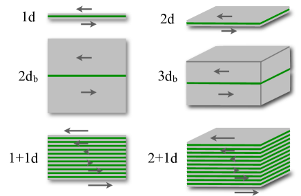
Figure 1: (Color online) Overview of the geometries considered in this work. The grey regions are the magnetic systems, while the green (dark) regions are the moving boundaries. The arrows indicate the motion of the subsystems.

Magnetic contributions to friction due to spin correlations have attracted increasing interest in recent years. One interesting aspect is the energy dissipation due to spin waves in magnetic force microscopy, where magnetic structures are investigated by moving a magnetic tip over a surface (Fusco et al., 2008; Magiera et al., 2009a, b). On the other hand, magnetic friction is also present in bulk magnetic systems which are in close proximity. In this context, Kadau et al. (Kadau et al., 2008) proposed a simple model for magnetic friction mediated solely by spin degrees of freedom. In this model an Ising spin system is moved over a second spin system with constant velocity $v$ along a boundary. This permanent perturbation drives the system to a steady state far away from equilibrium, leading to a permanent energy flow from the boundary to the heat bath.

This problem can be analyzed for several different geometries in one, two and three dimensions, as shown in Fig. 1: Besides the original problem of two half-infinite two dimensional systems moving along the one dimensional boundary, denoted $2\mathrm{d}_{\mathrm{b}}$ in the following, we will consider the homogeneous cases $1\mathrm{d}$ and $2\mathrm{d}$ where all spins are at the boundary, as well as the experimentally relevant three dimensional case $3\mathrm{d}_{\mathrm{b}}$. Additionally, we will extend the analysis to sheared systems in two (Chan and Lin, 1990; Corberi et al., 1998; Cirillo et al., 2005) and three (Imaeda and Kawasaki, 1984) dimensions, denoted $1{+}1\mathrm{d}$ and $2{+}1\mathrm{d}$. These systems are experimentally accessible within the framework of shear flow in binary liquid mixtures (for a review, see (Onuki, 1997)), though with conserved order parameter, while we deal with a non–conserved order parameter.

This model has some similarities to the driven lattice gas (DLG) proposed by Katz et al. (Katz et al., 1983) (see (Schmittmann and Zia, 1995) for a review), where a system is driven out of equilibrium by an applied field which favors the motion of particles in one direction. We will discuss these similarities throughout this work.

The paper is organized as follows: In the first part we will introduce the model and geometries and present, in the second part, an exact solution of the model in the limit of high driving velocities $v\rightarrow\infty$, which will be checked numerically in the last part using Monte Carlo simulations. There we will also investigate the case of finite velocities $v$.

II Model

Let us start with the simplest case denoted $1\mathrm{d}$ in Fig. 1 and consider two Ising chains with spin variables $\sigma=\pm 1$, nearest neighbor coupling $K=\beta J$ ($\beta=1/k_{\mathrm{B}}T$ and we set $k_{\mathrm{B}}=1$) and $L_{\parallel}$ sites each, interacting with boundary coupling $K_{\mathrm{b}}=\beta J_{\mathrm{b}}$ and moving along each other with relative velocity $v$. In the Monte Carlo simulation the upper system is moved $v$ times by one lattice constant $a_{0}$ with respect to the lower system during each random sequential Monte Carlo sweep (MCS). As one MCS corresponds to a typical spin relaxation time $t_{0}=\mathcal{O}(10^{-8}\mathrm{s})$ (Stearns, 1986) and $a_{0}=\mathcal{O}(10^{-10}\mathrm{m})$, the velocity $v$ is given in natural units $a_{0}/t_{0}=\mathcal{O}(1\mathrm{cm/s})$ (we will set $a_{0}=t_{0}=1$ in the following).

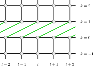
Figure 2: (Color online) Sketch of geometry $1\mathrm{d}$ after $\Delta=2$ moves. Spin $\sigma_{0,l}$ interacts with spin $\sigma_{1,l+2}$ with coupling $J_{\mathrm{b}}$ (green (gray) lines), while all other couplings are $J$ (black lines).

To simplify the implementation, instead of moving the upper part of the lattice with respect to the lower part we reorder the couplings at the boundary with time. This procedure is analogous to the Lees–Edwards or moving boundary condition in molecular dynamics simulations of fluids (Allen and Tildesley, 1987) and leads to a system as shown in Fig. 2. Assuming periodic boundary conditions (PBC) $\sigma_{k,l}\equiv\sigma_{k,l\bmod L_{\parallel}}$ in the parallel direction, the time dependent Hamiltonian reads

$$\beta\mathcal{H}(t)=-K\sum_{k=0}^{1\vphantom{L_{\parallel}}}\sum_{l=1}^{L_{\parallel}}\sigma_{k,l}\sigma_{k,l+1}-K_{\mathrm{b}}\sum_{l=1}^{L_{\parallel}}\sigma_{0,l}\sigma_{1,l+\Delta(t)}$$ (1)

with the time dependent displacement

$$\Delta(t)=vt.$$ (2)

Figure 3: (Color online) Sketch of geometry $2\mathrm{d}_{\mathrm{b}}$ after $\Delta=2$ moves.

The second geometry considered in this work is the $2\mathrm{d}_{\mathrm{b}}$ case shown in Fig. 3, which already was investigated by Kadau et al. (Kadau et al., 2008). Here we have a square lattice with $L_{\parallel}\times L_{\perp}$ sites and periodic boundary conditions in both directions, i. e., $\sigma_{k,l}\equiv\sigma_{k\bmod L_{\perp},l\bmod L_{\parallel}}$. Note that especially $\sigma_{L_{\perp},l}\equiv\sigma_{0,l}$. The Hamiltonian of this system becomes

$$\beta\mathcal{H}(t)=-\sum_{k=1}^{L_{\perp}\vphantom{L_{\parallel}}}\sum_{l=1}^{L_{\parallel}}K\sigma_{k,l}\sigma_{k,l+1}+K_{\perp,k}\sigma_{k,l}\sigma_{k+1,l+\Delta_{k}(t)}$$ (3)

with $\Delta_{k}(t)\equiv 0$ and $K_{\perp,k}=K$ for all rows except row $k=0$, where the couplings to row $k=1$ are shifted with constant velocity $\Delta_{0}(t)\equiv\Delta(t)=vt.$ The coupling $K_{\perp,0}\equiv K_{\mathrm{b}}$ across the boundary is allowed to be different from $K$. For $v=0$ and $J_{\mathrm{b}}=J=1$ this system simplifies to the $2d$ Ising model in equilibrium, which was solved exactly by Onsager (1944) and shows a continuous phase transition at

$$T_{\mathrm{c,eq}}=\frac{2}{\log(1+\sqrt{2})}=2.2691853\ldots\,.$$ (4)

Note that both systems are translationally invariant in $\parallel$ direction under the transformation $l\rightarrow l+1$ and obey reflection symmetry at the boundary under $k\rightarrow 1-k$.

III Exact solution at high velocities

In Ref. (Kadau et al., 2008) it was shown that for high velocities $v\gg 1$ the properties of the $2\mathrm{d}_{\mathrm{b}}$ system become independent of $v$. This can be understood as follows: In the limit $v\rightarrow\infty$ the interaction $K_{\mathrm{b}}\sigma_{0,l}\sigma_{1,l+\Delta(t)}$ across the driven boundary becomes uncorrelated, as, in the Monte Carlo simulations, at large $v$ the spin $\sigma_{1,l+\Delta(t)}$ is different in every trial step and can, for simplicity, be a randomly chosen spin $\sigma_{1,\mathrm{rnd}}$ from row $1$. Note that this simplification was checked within the simulations and indeed gave the same results, enabling us to perform simulations at $v=\infty$. Thus the boundary coupling can be replaced by the action of a fluctuating boundary field $\mu$, e.g.,

$$\sigma_{0,l}\sigma_{1,l+\Delta(t)}\rightarrow\sigma_{0,l}\sigma_{1,\mathrm{rnd}}\rightarrow\sigma_{0,l}\mu_{0,l},$$ (5)

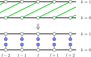
with stochastic variables $\mu_{kl}=\pm 1$ ($k=0,1$) under the constraint $\langle\mu_{kl}\rangle=\langle\sigma_{kl}\rangle=m_{\mathrm{b}}$, where $m_{\mathrm{b}}$ denotes the magnetization at the driven boundary. Here we used the translation symmetry $\langle\sigma_{kl}\rangle=m_{k}$ and the reflection symmetry at the boundary, $m_{k}=m_{1-k}$. In Fig. 4 this mapping of the driven system onto a system with fluctuating boundary fields is illustrated for the $1\mathrm{d}$ case. The next step will be to map the fluctuating fields onto static fields by integrating out the degrees of freedom $\mu_{kl}$.

III.1 Ising model in a fluctuating field

Figure 4: (Color online) Mapping of the $1\mathrm{d}$ driven system, shown for $\Delta=2$, on two disconnected $1d$ systems with fluctuating fields.

Consider a general Ising model with arbitrary couplings $K_{ij}$ in a static external field $h_{i}^{\mathrm{ext}}$ and additional fluctuating fields of strength $k_{i}$ (note the factor $\beta$ in all field quantities)

$$\beta\mathcal{H}_{\mu}=-\sum_{i<j}K_{ij}\sigma_{i}\sigma_{j}-\sum_{i}(h_{i}^{\mathrm{ext}}+k_{i}\mu_{i})\sigma_{i}$$ (6)

where the $\mu_{i}=\pm 1$ are stochastic variables at site $i$ with given average

$$\langle\mu_{i}\rangle=m_{i}.$$ (7)

As this condition is given a priori, averages containing $\mu_{i}$ can be calculated using the trace formula

$$\mathop{\operator@font Tr}\nolimits_{\mu}f(\mu_{i})=\sum_{\mu_{i}=\pm 1}f(\mu_{i})p_{i}(\mu_{i})$$ (8)

with the probability distribution $p_{i}(\mu_{i})=(1+\mu_{i}m_{i})/2$, as then

$$\langle\mu_{i}\rangle=\mathop{\operator@font Tr}\nolimits_{\mu}\mu_{i}=\sum_{\mu_{i}=\pm 1}\mu_{i}\,p_{i}(\mu_{i})=m_{i}$$

as assumed. With the decomposition

$$\beta\mathcal{H}_{\mu}=\beta\mathcal{H}_{0}-\sum_{i}k_{i}\mu_{i}\sigma_{i}$$ (9)

the degrees of freedom $\mu$ in the partition function $\mathcal{Z}$ can be traced out,

$$\mathcal{Z} = \mathop{\operator@font Tr}\nolimits_{\sigma\mu}e^{-\beta\mathcal{H}_{\mu}}\>=\>\mathop{\operator@font Tr}\nolimits_{\sigma}e^{-\beta\mathcal{H}_{0}}\mathop{\operator@font Tr}\nolimits_{\mu}\prod_{i}e^{k_{i}\mu_{i}\sigma_{i}}$$ (10)

$$= \mathop{\operator@font Tr}\nolimits_{\sigma}e^{-\beta\mathcal{H}_{0}}\prod_{i}\sum_{\mu_{i}=\pm 1}e^{k_{i}\mu_{i}\sigma_{i}}p_{i}(\mu_{i})$$

$$= \prod_{i}\cosh k_{i}\mathop{\operator@font Tr}\nolimits_{\sigma}e^{-\beta\mathcal{H}_{0}}\prod_{i}\left[1+\sigma_{i}m_{i}\tanh k_{i}\right],$$

where we used the fact that $\sigma_{i}=\pm 1$.

On the other hand, the Hamiltonian of the equilibrium Ising model without fluctuating fields in a static field $h_{i}$ can be written as

$$\beta\mathcal{H}_{\mathrm{eq}}=-\sum_{i<j}K_{ij}\sigma_{i}\sigma_{j}-\sum_{i}h_{i}\sigma_{i}=\beta\mathcal{H}_{0}-\sum_{i}b_{i}\sigma_{i}$$ (11)

with $\mathcal{H}_{0}$ from Eq. (9), if we let $b_{i}=h_{i}-h_{i}^{\mathrm{ext}}$. The partition function of this model clearly fulfills

$$\mathcal{Z}_{\mathrm{eq}} = \mathop{\operator@font Tr}\nolimits_{\sigma}e^{-\beta\mathcal{H}_{\mathrm{eq}}}\>=\>\mathop{\operator@font Tr}\nolimits_{\sigma}e^{-\beta\mathcal{H}_{0}}\prod_{i}e^{b_{i}\sigma_{i}}$$ (12)

$$= \prod_{i}\cosh b_{i}\mathop{\operator@font Tr}\nolimits_{\sigma}e^{-\beta\mathcal{H}_{0}}\prod_{i}\left[1+\sigma_{i}\tanh b_{i}\right].$$

Comparing Eqs. (10) and (12), we conclude that under the condition

$$\tanh b_{i}=m_{i}\tanh k_{i}$$ (13)

the partition function $\mathcal{Z}$ can be expressed in terms of $\mathcal{Z}_{\mathrm{eq}}$,

$$\mathcal{Z}=\left.\prod_{i}\frac{\cosh k_{i}}{\cosh b_{i}}\,\mathcal{Z}_{\mathrm{eq}}\right|_{\mathrm{Eq.\,(\ref{eq:condition})}}.$$ (14)

To summarize, the coupling with strength $k_{i}$ to fluctuating fields $\mu_{i}=\pm 1$ with given average $\langle\mu_{i}\rangle=m_{i}$ can be written as coupling to static effective fields $b_{i}$ with strength given by Eq. (13). In the next section we will use this mapping to exactly solve the driven Ising model for high velocities $v\rightarrow\infty$.

III.2 Application to the driven Ising model

The general condition Eq. (13) for the effective static fields $b_{i}$ simplifies for the systems considered in this work: As all boundary spins are equivalent, $m_{i}=m_{\mathrm{b}}$, with coupling $k_{i}=K_{\mathrm{b}}$, leading to a uniform effective field $h_{\mathrm{b}}=\mathop{\operator@font artanh}\nolimits(m_{\mathrm{b}}\tanh K_{\mathrm{b}})$ at the boundary, as we assume no additional external fields, $h_{i}^{\mathrm{ext}}=0$. Inserting this into the equilibrium expression for the boundary magnetization $m_{\mathrm{b},\mathrm{eq}}(K,h_{\mathrm{b}})=\partial\ln\mathcal{Z}_{\mathrm{eq}}/\partial h_{\mathrm{b}}$, we end with the self–consistence condition

$$m_{\mathrm{b},\mathrm{eq}}[K,\mathop{\operator@font artanh}\nolimits(m_{\mathrm{b}}\tanh K_{\mathrm{b}})]=m_{\mathrm{b}}$$ (15)

for the non–equilibrium order parameter $m_{\mathrm{b}}$.

As $1=\partial m_{\mathrm{b},\mathrm{eq}}/\partial m_{\mathrm{b}}|_{m_{\mathrm{b}}=0}$ at criticality, we obtain a very useful connection between the reduced zero field boundary susceptibility of the equilibrium model $\chi_{\mathrm{b},\mathrm{eq}}^{(0)}(K)=\partial m_{\mathrm{b},\mathrm{eq}}/\partial h_{\mathrm{b}}|_{h_{\mathrm{b}}=0}$ and the critical temperature $T_{\mathrm{c}}$ of the driven system by expanding Eq. (15) to first order around $m_{\mathrm{b}}=0$, namely

$$\chi_{\mathrm{b},\mathrm{eq}}^{(0)}(K_{\mathrm{c}})\,\tanh K_{\mathrm{b},\mathrm{c}}=1.$$ (16)

In the following we will apply these results to the one and two dimensional model introduced in Section II.

III.3 1d case

The effective Hamiltonian of the system $1\mathrm{d}$ in a fluctuating field reads

$$\beta\mathcal{H}=-\sum_{l=1}^{L_{\parallel}}K\sigma_{l}\sigma_{l+1}+(h^{\mathrm{ext}}+K_{\mathrm{b}}\mu_{l})\sigma_{l}.$$ (17)

Applying the self–consistence condition Eq. (15) to the well known expression for the equilibrium magnetization of the $1d$ Ising model (cf. Baxter, 1982)

$$m_{\mathrm{eq}}(K,h)=\frac{\sinh h}{\sqrt{e^{-4K}+\sinh^{2}h}}$$ (18)

we obtain the zero field magnetization of the $1\mathrm{d}$ driven system in the ordered phase for velocity $v\rightarrow\infty$,

$$m(K,K_{\mathrm{b}})=\sqrt{\frac{\cosh 2K_{\mathrm{b}}-\coth 2K}{\cosh 2K_{\mathrm{b}}-1}}$$ (19)

with critical temperature fulfilling

$$e^{2K_{\mathrm{c}}}\tanh K_{\mathrm{b},\mathrm{c}}=1,$$ (20)

as $\chi_{\mathrm{eq}}^{(0)}(K)=e^{2K}$ in this case. Interestingly, Eq. (19) is equal to the spontaneous surface magnetization of the $2d$ equilibrium Ising model (McCoy and Wu, 1973, Chapter VI, Eq. 5.20) if we identify $K$ and $K_{\mathrm{b}}$ with the couplings $\parallel$ and $\perp$ to the surface, and consequently has the identical critical temperature $T_{\mathrm{c}}$. For the special case $K=K_{\mathrm{b}}$ this gives the well known value from Eq. (4). However, we regard this equality as coincidence without deeper meaning, as Eq. (19) is solution of a simple quadratic equation with small integer coefficients when written in the natural variables. Nevertheless, we checked this identity in the $2\mathrm{d}$ case and found that we do not get the surface magnetization of the $3d$ system by the same procedure, as the critical temperature is $T_{\mathrm{c}}\approx 4.058$ (Eq. (60)) instead of the correct value $T_{\mathrm{c}}=4.511424(53)$ (Ferrenberg and Landau, 1991; Ito et al., 2000).

To calculate other quantities we use the transfer matrix (TM) formulation: the TM of the $1d$ equilibrium Ising model reads (cf. Baxter, 1982)

$$\mathbf{T}_{\mathrm{eq}}=\left(\begin{array}[]{cc}e^{K+h}&e^{-K}\\ e^{-K}&e^{K-h}\end{array}\right)$$ (21)

and the partition function of a periodic system with $L_{\parallel}$ spins can be expressed as

$$\mathcal{Z}_{\mathrm{eq}}=\mathop{\operator@font Tr}\nolimits\mathbf{T}_{\mathrm{eq}}^{L_{\parallel}}.$$ (22)

Using Eq. (14) and the conditions Eq. (13) we can write

$$\mathcal{Z}=\mathop{\operator@font Tr}\nolimits\mathbf{T}^{L_{\parallel}}$$ (23)

with the TM (we set $h^{\mathrm{ext}}=0$ from now on)

$$\mathbf{T}=\left.\frac{\cosh K_{\mathrm{b}}}{\cosh h}\,\mathbf{T}_{\mathrm{eq}}\right|_{\tanh h=m\tanh K_{\mathrm{b}}},$$ (24)

which can be written as

$$\mathbf{T}=\cosh K_{\mathrm{b}}\left(\begin{array}[]{cc}e^{K}\left(1+\sin\psi\right)&e^{-K}\cos\psi\\ e^{-K}\cos\psi&e^{K}\left(1-\sin\psi\right)\end{array}\right)$$ (25)

using

$$\sin\psi=m\tanh K_{\mathrm{b}}.$$ (26)

The angle $\psi$ decreases from $\psi=\pi/2$ at $T=0$ to $\psi=0$ at $T\geq T_{\mathrm{c}}$. The eigenvalues $\lambda_{\mu}$ of $\mathbf{T}$ fulfill

$$\mathbf{T}|t_{\mu}\rangle=\lambda_{\mu}|t_{\mu}\rangle$$ (27)

and are given by

$$\lambda_{0,1}=\left\{\begin{array}[]{lll}{\displaystyle e^{K\pm K_{\mathrm{b}}}}&&T\leq T_{\mathrm{c}}\\ {\displaystyle\cosh K_{\mathrm{b}}(e^{K}\pm e^{-K})}&&T\geq T_{\mathrm{c}}\end{array}\right.$$ (28)

where $\lambda_{0}$ denotes the larger eigenvalue dominant in the thermodynamic limit. Note that in this limit the analog to the free energy density

$$f=-\frac{1}{\beta}\log\lambda_{0}=-(J+J_{\mathrm{b}})$$ (29)

of the driven system is simply a constant in the ordered phase $T\leq T_{\mathrm{c}}$ . Nevertheless, we can calculate physical quantities within this TM notation using expectation values, as the whole information of the half-infinite system is contained in the normalized eigenvectors

$$|t_{0}\rangle=\left(\begin{array}[]{c}\cos\phi\\ \sin\phi\end{array}\right),\;|t_{1}\rangle=\left(\begin{array}[]{c}-\sin\phi\\ \hphantom{-}\cos\phi\end{array}\right)$$ (30)

with $\cos 2\phi=m$. Using the normalized TM $\hat{\mathbf{T}}=\mathbf{T}/\lambda_{0}$ and the Pauli matrix $\mathbf{M}=\mathop{\operator@font diag}\nolimits(1,-1)$, the magnetization, Eq. (19), can be expressed as

$$m=\langle t_{0}|\mathbf{M}|t_{0}\rangle,$$ (31)

while the correlation function in $\parallel$ direction becomes

$$g_{\parallel}(n) = \langle\sigma_{l}\sigma_{l+n}\rangle-\langle\sigma_{l}\rangle\langle\sigma_{l+n}\rangle$$ (32)

$$= \langle t_{0}|\mathbf{M}\hat{\mathbf{T}}^{n}\mathbf{M}|t_{0}\rangle-\langle t_{0}|\mathbf{M}|t_{0}\rangle^{2}$$

$$= \lambda_{1}^{n}\lambda_{0}^{-n}\langle t_{0}|\mathbf{M}|t_{1}\rangle^{2},$$

as $\mathbf{T}^{n}=\sum_{\mu}\lambda_{\mu}^{n}|t_{\mu}\rangle\langle t_{\mu}|$. We get the result

$$g_{\parallel}(n)=\left\{\begin{array}[]{lll}{\displaystyle(1-m^{2})e^{-2nK_{\mathrm{b}}}}&&T\leq T_{\mathrm{c}}\\ {\displaystyle\tanh^{n}K}&&T\geq T_{\mathrm{c}}\end{array}\right.,$$ (33)

leading to the inverse correlation length

$$\xi_{\parallel}^{-1}=\log\frac{\lambda_{0}}{\lambda_{1}}=\left\{\begin{array}[]{lll}{\displaystyle 2K_{\mathrm{b}}}&&T\leq T_{\mathrm{c}}\\ {\displaystyle\log\coth K}&&T\geq T_{\mathrm{c}}\end{array}\right..$$ (34)

Note that $\xi_{\parallel}$ does not diverge at the critical point, a feature which would lead to a correlation length exponent $\nu=0$. In Section IV we will argue that in finite systems the spin fluctuations are not only mediated by the spins $\sigma_{i}$ but also by the self consistent field $m$ which fluctuates at finite $L_{\parallel}$, an effect which vanishes in the exact solution, as $L_{\parallel}\to\infty$.

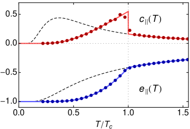
Figure 5: (Color online) Internal energy $e_{\parallel}(T)$, Eq. (35), and specific heat $c_{\parallel}(T)$, Eq. (36), of the $1\mathrm{d}$ driven system at $v\to\text{$\infty$}$. The points are MC results for $L_{\parallel}=2^{11}$, and the dashed lines are results for the one dimensional Ising model in equilibrium.

From the nearest neighbor correlation function we can calculate the internal energy $e_{\parallel}=-J\langle\sigma_{l}\sigma_{l+1}\rangle$ in $\parallel$ direction

$$e_{\parallel}=\left\{\begin{array}[]{lll}{\displaystyle\frac{Je^{-2K-K_{\mathrm{b}}}}{\sinh 2K\sinh K_{\mathrm{b}}}-1}&&T\leq T_{\mathrm{c}}\\ \\ {\displaystyle-J\tanh K}&&T\geq T_{\mathrm{c}}\end{array}\right.$$ (35)

as well as the specific heat $c_{\parallel}=\partial e_{\parallel}/\partial T$ in $\parallel$ direction

$$c_{\parallel}=\left\{\begin{array}[]{lll}{\displaystyle\frac{2K^{2}}{\sinh^{2}K}(\coth K_{\mathrm{b}}-1)}&&T<T_{\mathrm{c}}\\ \\ {\displaystyle\frac{K^{2}}{\cosh^{2}K}}&&T>T_{\mathrm{c}}\end{array}\right..$$ (36)

On the other hand, the internal energy in $\perp$ direction is simply given by

$$e_{\perp}=-J_{\mathrm{b}}m^{2}$$ (37)

as the related spins are uncorrelated.

Now we turn to dynamical properties of this system under a concrete MC Glauber dynamics (see Sec. IV.2 for details) and calculate the spin flip acceptance rate $A=\langle p_{\mathrm{flip}}\rangle$ and the energy dissipation rate $P=\partial E/\partial t$: Let $\langle\zeta_{\ell}\,\zeta\,\zeta_{r}\rangle$ denote the probability of picking a spin $\sigma$ with direction $\zeta=\uparrow,\downarrow$ and left and right neighbors $\sigma_{\ell,r}$ with direction $\zeta_{\ell,r}$. These probabilities can be calculated using the matrices $\mathbf{P}_{\uparrow}=\mathop{\operator@font diag}\nolimits(1,0)$ and $\mathbf{P}_{\downarrow}=\mathop{\operator@font diag}\nolimits(0,1)$, e. g., $\langle\uparrow\uparrow\downarrow\rangle=\langle t_{0}|\mathbf{P}_{\uparrow}\hat{\mathbf{T}}\mathbf{P}_{\uparrow}\hat{\mathbf{T}}\mathbf{P}_{\downarrow}|t_{0}\rangle$. As the third coupling partner $\mu$ of spin $\sigma$, with direction $\zeta_{\mu}$, is uncorrelated at infinite velocity, the probability of a particular spin configuration becomes

$$\langle\zeta_{\ell}\,\zeta\,\zeta_{r}\rangle\langle\zeta_{\mu}\rangle=\langle t_{0}|\mathbf{P}_{\zeta_{\ell}}\hat{\mathbf{T}}\mathbf{P}_{\zeta}\hat{\mathbf{T}}\mathbf{P}_{\zeta_{r}}|t_{0}\rangle\langle t_{0}|\mathbf{P}_{\zeta_{\mu}}|t_{0}\rangle.$$ (38)

The spin flip probability of a given configuration is $p_{\mathrm{flip}}(\Delta E)$, with $\Delta E=\Delta E_{1}+\Delta E_{2}=2J\sigma(\sigma_{\ell}+\sigma_{r})+2J_{\mathrm{b}}\sigma\mu$, and $A$ becomes the sum over all $2^{4}$ possible cases

$$A=\sum_{\zeta_{\ell},\zeta,\zeta_{r},\zeta_{\mu}=\uparrow,\downarrow}p_{\mathrm{flip}}(\Delta E)\langle\zeta_{\ell}\,\zeta\,\zeta_{r}\rangle\langle\zeta_{\mu}\rangle,$$ (39)

which can be written as

$$A = \sum_{\zeta_{\ell},\zeta,\zeta_{r}=\uparrow,\downarrow}p_{\mathrm{flip}}^{*}(\Delta E_{1})\langle\zeta_{\ell}\,\zeta\,\zeta_{r}\rangle\sum_{\zeta_{\mu}=\uparrow,\downarrow}p_{\mathrm{flip}}^{*}(\Delta E_{2})\langle\zeta_{\mu}\rangle$$ (40)

$$= \sum_{\zeta=\uparrow,\downarrow}X_{\zeta}\left(e^{-2K_{\mathrm{b}}}\langle\zeta\rangle+\langle\bar{\zeta}\rangle\right)$$

for the multiplicative rate $p_{\mathrm{flip}}^{*}(\Delta E)=p_{\mathrm{flip}}^{*}(\Delta E_{1})p_{\mathrm{flip}}^{*}(\Delta E_{2})$ introduced in Sec. IV.2, Eq. (69), using the abbreviation

$$X_{\zeta} = \sum_{\zeta_{\ell},\zeta_{r}=\uparrow,\downarrow}p_{\mathrm{flip}}^{*}(\Delta E_{1})\langle\zeta_{\ell}\,\zeta\,\zeta_{r}\rangle$$ (41)

$$= e^{-4K}\langle\zeta\zeta\zeta\rangle+2e^{-2K}\langle\zeta\zeta\bar{\zeta}\rangle+\langle\bar{\zeta}\zeta\bar{\zeta}\rangle.$$

Note that the two terms in Eq. (40) are equal and the acceptance rate is independent of spin $\zeta$ because $m$ is stationary. The resulting acceptance rate becomes

$$A=\left\{\begin{array}[]{lll}{\displaystyle\frac{\cosh(K+K_{\mathrm{b}})-\sinh(K-K_{\mathrm{b}})}{4e^{2(K+K_{\mathrm{b}})}\sinh K\cosh^{2}K\sinh K_{\mathrm{b}}}}&&T\leq T_{\mathrm{c}}\\ \\ e^{-K_{\mathrm{b}}}\cosh K_{\mathrm{b}}(1-\tanh K)^{2}&&T\geq T_{\mathrm{c}}\end{array}\right.,$$ (42)

which simplifies for $J=J_{\mathrm{b}}$ to

$$A=\left\{\begin{array}[]{lll}{\displaystyle\frac{e^{-4K}\coth 2K}{\sinh 2K}}&&T\leq T_{\mathrm{c}}\\ \\ {\displaystyle\frac{e^{-3K}}{\cosh K}}&&T\geq T_{\mathrm{c}}\end{array}\right..$$ (43)

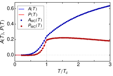
Figure 6: (Color online) Spin flip probability $A$, Eq. (43), and energy dissipation rate $P$, Eq. (47), versus reduced temperature $T/T_{\mathrm{c}}$ for the $1\mathrm{d}$ system at $v\to\infty$, together with MC data for $L_{\parallel}=2^{11}$.

The calculation of the energy dissipation rate $P$ per spin is very similar to the acceptance rate $A$ (Eq. (40)) and gives

$$P=-2J_{\mathrm{b}}\sum_{\zeta=\uparrow,\downarrow}X_{\zeta}\left(e^{-2K_{\mathrm{b}}}\langle\zeta\rangle-\langle\bar{\zeta}\rangle\right).$$ (44)

Furthermore, $P/A$ can be calculated for arbitrary dimensions and geometries, as it is solely a property of the fluctuating field. We find

$$\frac{P}{A} = -2J_{\mathrm{b}}\frac{\sum_{\zeta=\uparrow,\downarrow}X_{\zeta}\left(e^{-2K_{\mathrm{b}}}\langle\zeta\rangle-\langle\bar{\zeta}\rangle\right)}{\sum_{\zeta=\uparrow,\downarrow}X_{\zeta}\left(e^{-2K_{\mathrm{b}}}\langle\zeta\rangle+\langle\bar{\zeta}\rangle\right)}$$ (45)

$$= -J_{\mathrm{b}}\sum_{\zeta=\uparrow,\downarrow}\frac{e^{-2K_{\mathrm{b}}}\langle\zeta\rangle-\langle\bar{\zeta}\rangle}{e^{-2K_{\mathrm{b}}}\langle\zeta\rangle+\langle\bar{\zeta}\rangle}$$

$$= \frac{2J_{\mathrm{b}}(m^{2}+1)\tanh K_{\mathrm{b}}}{1-m^{2}\tanh^{2}K_{\mathrm{b}}}.$$

For the magnetization Eq. (19) of the $1\mathrm{d}$ system this gives

$$\frac{P}{A}=\left\{\begin{array}[]{lll}{\displaystyle\frac{2J_{\mathrm{b}}e^{-4K}}{\tanh K_{\mathrm{b}}}}&&T\leq T_{\mathrm{c}}\\ \\ 2J_{\mathrm{b}}\tanh K_{\mathrm{b}}&&T\geq T_{\mathrm{c}}\end{array}\right.,$$ (46)

which, multiplied with $A$ from Eq. (71) and for $J=J_{\mathrm{b}}$, becomes

$$P=\left\{\begin{array}[]{lll}{\displaystyle\frac{2e^{-8K}\coth 2K}{\tanh K\sinh 2K}}&&T\leq T_{\mathrm{c}}\\ \\ {\displaystyle\frac{2e^{-3K}\tanh K}{\cosh K}}&&T\geq T_{\mathrm{c}}\end{array}\right..$$ (47)

These results are shown in Fig. 6, together with data from MC simulations. Note that these results are only valid for the multiplicative rate $p_{\mathrm{flip}}^{*}$ from Eq. (69).

Finally we list the critical exponents for the $1\mathrm{d}$ driven system at $v\to\infty$ to be

$$\beta=\frac{1}{2},\;\gamma=1,\;\alpha=0.$$ (48)

The behavior of this system at finite velocities $v$ will be discussed in Sec. IV.

III.4 2d_b case

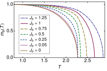
Figure 7: (Color online) Boundary magnetization $m_{\mathrm{b}}(T)$, Eq. (49), of the $2\mathrm{d}_{\mathrm{b}}$ system for $J=1$ and several values of $J_{\mathrm{b}}$. For $J_{\mathrm{b}}=0$ the $m_{\mathrm{b}}$ reduces to the surface magnetization of the $2d$ equilibrium Ising model, Eq. (80).

The $2\mathrm{d}_{\mathrm{b}}$ case can be solved exactly using the expression for the equilibrium surface magnetization $m_{\mathrm{b},\mathrm{eq}}(z,y_{\mathrm{b}})$ of the $2d$ Ising model in a static surface field $h_{\mathrm{b}}$ obtained by McCoy and Wu (McCoy and Wu, 1973, Chapter VI, Eq. 5.1), with $z=\tanh K$ and $y_{\mathrm{b}}=\tanh h_{\mathrm{b}}$. The integral representation given in their work can be further evaluated and written in closed form, the results are given in Appendix A, Eq. (77). If we again use Eq. (15) and set $y_{\mathrm{b}}=m_{\mathrm{b}}z_{\mathrm{b}}$, with $z_{\mathrm{b}}=\tanh K_{\mathrm{b}}$, we can calculate the non–equilibrium boundary magnetization $m_{\mathrm{b}}(z,z_{\mathrm{b}})$ numerically as solution of the self–consistence condition

$$m_{\mathrm{b},\mathrm{eq}}(z,m_{\mathrm{b}}z_{\mathrm{b}})=m_{\mathrm{b}},$$ (49)

which is shown for $J=1$ and several values of $J_{\mathrm{b}}$ in Fig. 7. The critical temperature $T_{\mathrm{c}}$ of the system can be evaluated from the reduced zero field boundary susceptibility $\chi_{\mathrm{b},\mathrm{eq}}(z)$, Eq. (78), to give

$$T_{\mathrm{c}}=2.6614725655752\ldots$$ (50)

for the case $J_{\mathrm{b}}=J=1$ using $\chi_{\mathrm{b},\mathrm{eq}}^{(0)}(z_{\mathrm{c}})z_{\mathrm{b},\mathrm{c}}=1$ (Eq. (16)).

As the critical temperature $T_{\mathrm{c}}$, Eq. (50), is larger than the equilibrium critical temperature $T_{\mathrm{c,eq}}=2.26918\ldots$, the driven boundary induces a surface phase transition where only the driven surface has long range order above $T_{\mathrm{c,eq}}$. The velocity dependence of this transition and the resulting phase diagram is discussed in more detail in Section IV.

III.5 1+1d sheared case

If the motion of the lattice described by Eq. (3) is not restricted to one row but applied to the whole system we get a system with uniform shear. Then all $\Delta_{k}(t)\equiv\Delta(t)=vt$ are equal, and we assume $K_{\perp,k}\equiv K_{\perp}$ to get

$$\beta\mathcal{H}(t)=-\sum_{k=1}^{L_{\perp}\vphantom{L_{\parallel}}}\sum_{l=1}^{L_{\parallel}}K_{\parallel}\sigma_{k,l}\sigma_{k,l+1}+K_{\perp}\sigma_{k,l}\sigma_{k+1,l+\Delta(t)}.$$ (51)

Note that this system is translationally invariant in both directions, a fact that drastically simplifies the analysis of the critical behavior.

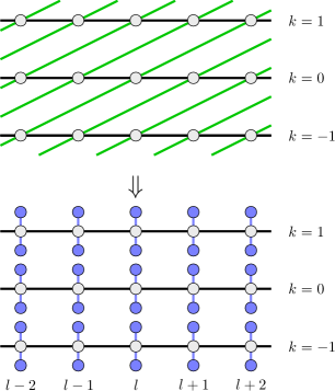
Figure 8: (Color online) Mapping of the $1{+}1\mathrm{d}$ sheared system, shown for $\Delta=2$, on $L_{\perp}$ disconnected $1d$ systems with fluctuating fields

Now we will investigate this system in the limit $v\rightarrow\infty$. Then each spin $\sigma_{kl}$ interacts, as depicted in Fig. 8, with its neighbors $\sigma_{k\pm 1,l\pm\Delta(t)}$ via fluctuating fields, while the interaction to the parallel neighbors $\sigma_{k,l\pm 1}$ remains unchanged. Thus the system decomposes into $L_{\perp}$ identical $1d$ Ising models which again can be solved exactly: The coupling to two fluctuating fields $\mu_{i,1}$ and $\mu_{i,2}$ with equal strength $k_{i}$ on each site can be traced similar to Eq. (10) to give

$$\mathcal{Z} = \mathop{\operator@font Tr}\nolimits_{\sigma}e^{-\beta\mathcal{H}_{0}}\mathop{\operator@font Tr}\nolimits_{\mu}\prod_{i}\prod_{j=1}^{2}e^{k_{i}\mu_{ij}\sigma_{i}}$$ (52)

$$= \mathop{\operator@font Tr}\nolimits_{\sigma}e^{-\beta\mathcal{H}_{0}}\prod_{i}\prod_{j=1}^{2}\sum_{\mu_{ij}=\pm 1}e^{k_{i}\mu_{ij}\sigma_{i}}p_{i}(\mu_{ij})$$

$$= \mathop{\operator@font Tr}\nolimits_{\sigma}e^{-\beta\mathcal{H}_{0}}\prod_{i}\left[\cosh k_{i}+m_{i}\sigma_{i}\sinh k_{i}\right]^{2}$$

$$= \prod_{i}C_{i}\mathop{\operator@font Tr}\nolimits_{\sigma}e^{-\beta\mathcal{H}_{0}}\prod_{i}\left[1+\sigma_{i}\frac{m_{i}}{C_{i}}\sinh 2k_{i}\right],$$

with

$$C_{i}=\frac{1}{2}\left(1-m_{i}^{2}+(1+m_{i}^{2})\cosh 2k_{i}\right).$$ (53)

Equating Eq. (52) with Eq. (12) we conclude that static fields $b_{i}$ can replace the fluctuating fields $\mu_{ij}$, with average $m_{i}$, if

$$\tanh b_{i}=\frac{2m_{i}\sinh 2k_{i}}{1-m_{i}^{2}+(1+m_{i}^{2})\cosh 2k_{i}}.$$ (54)

The sheared system is translationally invariant in both directions, leading to homogeneous values $m_{i}=m$, $k_{i}=K_{\perp}$, and $b_{i}=h$. Inserting Eq. (54) into Eq. (19) we get the order parameter of the sheared $1{+}1\mathrm{d}$ system

$$m(K_{\parallel},K_{\perp})\\ =\frac{\sqrt{1-2e^{4K_{\parallel}}+2e^{2K_{\parallel}}\sqrt{e^{4K_{\parallel}}-1+\tanh^{2}K_{\perp}}}}{\tanh K_{\perp}}$$ (55)

with critical temperature fulfilling

$$2e^{2K_{\parallel,\mathrm{c}}}\tanh K_{\perp,\mathrm{c}}=1,$$ (56)

which gives $T_{\mathrm{c}}=1/\log\left(\frac{1}{2}\sqrt{3+\sqrt{17}}\right)=3.46591...$ for $J_{\parallel}=J_{\perp}=1$. A generalization of Eq. (52) from two to $f$ fluctuating fields per spin is straightforward and leads to the general criticality condition

$$\chi_{\mathrm{eq}}^{(0)}(K_{\mathrm{c}})\,f\tanh K_{\mathrm{b},\mathrm{c}}=1.$$ (57)

Although this geometry can be solved exactly at $v=\infty$ we expect the phase transition to be strongly anisotropic (see, e. g., (Hucht, 2002)) with two different correlation length exponents $\nu_{\parallel}>\nu_{\perp}$. In fact we found such behavior, with strong evidence for the exponents $\nu_{\parallel}=3/2$ and $\nu_{\perp}=1/2$, details on this will be published elsewhere (Angst et al., 2010).

III.6 Other geometries

For two more cases we can derive highly accurate estimates for the critical temperature $T_{\mathrm{c}}$ of the driven system when $v\rightarrow\infty$, namely the $2\mathrm{d}$ Ising double layer (Angst et al., 2010) with Hamiltonian

$$\beta\mathcal{H}(t)=-\sum_{k=0}^{1\vphantom{L_{\parallel}}}\sum_{l=1}^{L_{\parallel}}\sum_{m=1}^{L_{\parallel}}\Bigl{[}K\sigma_{klm}(\sigma_{k,l,m+1}+\sigma_{k,l+1,m})+{}\\ {}+K_{\mathrm{b}}\sigma_{0lm}\sigma_{1,l+\Delta(t),m}\Bigr{]}$$ (58)

and the experimentally relevant $2{+}1\mathrm{d}$ sheared case

$$\beta\mathcal{H}(t)=-\sum_{k=1}^{L_{\perp}\vphantom{L_{\parallel}}}\sum_{l=1}^{L_{\parallel}}\sum_{m=1}^{L_{\parallel}}\Bigl{[}K_{\parallel}\sigma_{klm}(\sigma_{k,l,m+1}+\sigma_{k,l+1,m})+{}\\ {}+K_{\perp}\sigma_{klm}\sigma_{k+1,l+\Delta(t),m}\Bigr{]},$$ (59)

both on simple cubic lattices: With Eq. (57) we can express $T_{\mathrm{c}}$ using the high temperature series expansion for the reduced zero field susceptibility $\chi_{\mathrm{eq}}^{(0)}(K)$ of the $2d$ Ising model, which was calculated to higher than $2000^{\mathrm{th}}$ order recently using a highly efficient polynomial time algorithm (Boukraa et al., 2008). Using this extremely accurate result we find, for $J=J_{\mathrm{b}}=1$, the critical temperatures

$$T_{\mathrm{c}}=4.058782423137980000987775040680\ldots$$ (60)

for the two $2\mathrm{d}$ layers, and

$$T_{\mathrm{c}}=5.264750414514743550598017203424\ldots$$ (61)

for the $2{+}1\mathrm{d}$ sheared system with $f=2$ analogous to the $1{+}1\mathrm{d}$ sheared system. Note that due to the high accuracy of the series these values can be calculated to approximately $500$ and $700$ digits, respectively.

Just for reference we also give the critical temperatures for two more cases: The experimentally relevant $3\mathrm{d}_{\mathrm{b}}$ case shown in Fig. 1 as well as the quite theoretical $3\mathrm{d}$ case of two three dimensional systems in direct contact along the fourth dimension. In the $3\mathrm{d}_{\mathrm{b}}$ case we find $T_{\mathrm{c}}=4.8(1)$ using the $8^{\mathrm{th}}$ order high temperature series from Ref. (Binder and Hohenberg, 1974, Tab. IV), while in the $3\mathrm{d}$ case we obtain $T_{\mathrm{c}}=5.983835(1)$ using the $32^{\mathrm{th}}$ order series from (Arisue and Fujiwara, 2003).

All these higher dimensional geometries are expected to show strongly anisotropic behavior with two ($2\mathrm{d}$, $3\mathrm{d}_{\mathrm{b}}$ and $3\mathrm{d}$ case) or possibly even three different exponents ($2{+}1\mathrm{d}$ case), the reader is referred to Ref. (Angst et al., 2010).

IV Monte Carlo Simulations

IV.1 Method

We now describe the algorithms used to investigate the driven system: For finite velocities $v$ we shift the boundary couplings by increasing $\Delta(t)$ from Eq. (2) after every $N/v$ random sequential single spin flip attempts, where $N$ denotes the total number of spins. Using $10^{5}-10^{6}$ MCS per temperature, we measured the following boundary properties: The boundary magnetization per spin and the energy per bond parallel to and across the boundary of a given configuration

$$M_{\mathrm{b}} = \frac{1}{2L_{\parallel}}\sum_{k=0}^{1\vphantom{L_{\parallel}}}\sum_{l=1}^{L_{\parallel}}\sigma_{k,l}$$ (62a)

$$E_{\mathrm{b},\parallel} = -\frac{J}{2L_{\parallel}}\sum_{k=0}^{1\vphantom{L_{\parallel}}}\sum_{l=1}^{L_{\parallel}}\sigma_{k,l}\sigma_{k,l+1}$$ (62b)

$$E_{\mathrm{b}} = -\frac{J_{\mathrm{b}}}{L_{\parallel}}\sum_{l=1}^{L_{\parallel}}\sigma_{0,l}\sigma_{1,l+\Delta(t)}$$ (62c)

as well as the corresponding bulk quantities. From these time dependent quantities we calculate the averages of the magnetization, reduced susceptibility, Binder cumulant, internal energy and specific heat at the boundary,

$$m_{\mathrm{b},\mathrm{abs}} = \langle|M_{\mathrm{b}}|\rangle$$ (63a)

$$\chi_{\mathrm{b},\mathrm{abs}} = 2L_{\parallel}\left(\langle M_{\mathrm{b}}^{2}\rangle-\langle|M_{\mathrm{b}}|\rangle^{2}\right)$$ (63b)

$$U_{\mathrm{b}} = 1-\frac{\langle M_{\mathrm{b}}^{4}\rangle}{3\langle M_{\mathrm{b}}^{2}\rangle^{2}}$$ (63c)

$$e_{\mathrm{b}} = \langle E_{\mathrm{b}}\rangle$$ (63d)

$$c_{\mathrm{b}} = L_{\parallel}\beta^{2}\left(\langle E_{\mathrm{b}}^{2}\rangle-\langle E_{\mathrm{b}}\rangle^{2}\right).$$ (63e)

Note that we have absorbed the factor $\beta^{-1}$ into $\chi$. Near criticality these quantities show power law behavior and fulfill

$$m_{\mathrm{b},\mathrm{abs}}(\tau) \propto (-\tau)^{\beta}$$ (64a)

$$\chi_{\mathrm{b},\mathrm{abs}}(\tau) \propto |\tau|^{-\gamma}$$ (64b)

$$c_{\mathrm{b}}(\tau) \propto |\tau|^{-\alpha}$$ (64c)

with reduced temperature $\tau=T/T_{\mathrm{c}}-1$ and critical exponents $\beta$, $\gamma$ and $\alpha$. But, before we present the results, we have to take a closer look at the used spin flip rates.

IV.2 An integrable algorithm

While equilibrium properties are most efficiently investigated in Monte Carlo simulations using cluster algorithms, non–equilibrium systems have to be treated with random sequential single spin flip dynamics like the non-conserved Glauber dynamics (Glauber, 1963) or the conserved Kawasaki dynamics (Kawasaki, 1965). The driven system is permanently under an external perturbation which drives it out of equilibrium, while the internal degrees of freedom are coupled to a heat bath in thermal equilibrium. From this coupling the spin flip probability $p_{\mathrm{flip}}(\Delta E)$ of a given energy change $\Delta E$ fulfills the detailed balance condition

$$\frac{p_{\mathrm{flip}}(\Delta E)}{p_{\mathrm{flip}}(-\Delta E)}=e^{-\beta\Delta E}$$ (65)

just like in the equilibrium case (for details, see (Angst et al., 2010)).

The most common rates fulfilling Eq. (65) are the Metropolis rate (Metropolis et al., 1953) and the Glauber rate (Glauber, 1963),

$$p_{\mathrm{flip}}^{\mathrm{M}}(\Delta E) = \min(1,e^{-\beta\,\Delta E}),$$ (66a)

$$p_{\mathrm{flip}}^{\mathrm{G}}(\Delta E) = \frac{1}{1+e^{\beta\,\Delta E}}.$$ (66b)

Using these rates in simulations of, e. g., the $1\mathrm{d}$ driven system, Eq. (1), it turns out that for all $v>0$ the critical temperature $T_{\mathrm{c}}(v)$ depends on the used rate (see also Fig. 15): We find, for $v\to\infty$ and $J_{\mathrm{b}}=J=1$, the values $T_{\mathrm{c}}^{\mathrm{M}}=1.910(2)$ and $T_{\mathrm{c}}^{\mathrm{G}}=2.031(2)$ for the Metropolis and Glauber rate, respectively, while the exact solution Eq. (20) of the model presented in Section III gives $T_{\mathrm{c}}=2.269...$. Note that a similar dependency was recently found in the DLG by Kwak et al. (Kwak et al., 2004).

Figure 9: (Color online) Interactions of surface spin $\sigma_{i}$ in the $1\mathrm{d}$ case

How can these discrepancies be understood? And can we construct a rate that matches the analytical treatment, i. e., has the same $T_{\mathrm{c}}$? This is indeed possible: Consider a microscopic change, i. e. a spin flip, of spin $\sigma_{i}$ at the boundary (see Fig. 9), with energy difference

$$\Delta E=\underbrace{2J\sigma_{i}\sum\nolimits_{\langle j\rangle^{\prime}}^{z}\sigma_{j}}_{\Delta E_{1}}+\underbrace{2J_{\mathrm{b}}\sigma_{i}\vphantom{\sum\nolimits_{\langle j\rangle^{\prime}}}\sigma_{r}}_{\Delta E_{2}},$$ (67)

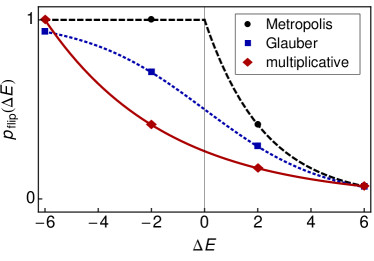
where the sum runs over the $z$ neighbors of $\sigma_{i}$ in the same subsystem ($z=2$ in the $1\mathrm{d}$ case), while $\sigma_{r}$ is from the other side of the moving boundary. The idea of the exact solution presented in the last section was to treat spin $\sigma_{r}$ as a fluctuating variable $\mu_{i}$ at site $i$ with appropriate statistics. By contrast, correlations of different strength are introduced between the two subsystems by the rates Eq. (66), because the influence of spin $\sigma_{r}$ depends on the actual state of the $z$ spins $\sigma_{j}$. This can be seen most easily in the case of the Metropolis rate ($J_{\mathrm{b}}=J$): if, e.g., $\sigma_{i}=-\sigma_{j}$ then $\Delta E_{1}=-2zJ$ and $p_{\mathrm{flip}}^{\mathrm{M}}=1$ independent of $\sigma_{r}$ (note that $\Delta E_{2}=\pm 2J$), while in the parallel case ($\sigma_{i}=\sigma_{j}$) $\Delta E_{1}=2zJ$ and $p_{\mathrm{flip}}^{\mathrm{M}}$ strongly depends on $\sigma_{r}$ (see Fig. 10).

Figure 10: (Color online) Spin flip probabilities of the Metropolis rate Eq. (66a) (dashed black line, circles), the Glauber rate Eq. (66b) (dotted blue line, squares), and the multiplicative rate Eq. (69) (red line, diamonds) for the $1\mathrm{d}$ system at criticality ($J=J_{\mathrm{b}}=1$).

Fortunately, these rate-induced correlations can be completely eliminated by requiring that the flipping probability is multiplicative,

$$p_{\mathrm{flip}}(\Delta E_{1}+\Delta E_{2})=p_{\mathrm{flip}}(\Delta E_{1})\,p_{\mathrm{flip}}(\Delta E_{2}).$$ (68)

Clearly this condition is not satisfied for the rates in Eq. (66), e. g., $p_{\mathrm{flip}}^{\mathrm{M}}(-2zJ+2J)=1$, while $p_{\mathrm{flip}}^{\mathrm{M}}(-2zJ)p_{\mathrm{flip}}^{\mathrm{M}}(2J)=e^{-2K}$ (again we assume $J_{\mathrm{b}}=J$).

Instead, for simulations of driven systems we propose the rate

$$p_{\mathrm{flip}}^{*}(\Delta E)=e^{-\frac{\beta}{2}(\Delta E-\Delta E_{\mathrm{min}})}$$ (69)

which is uniquely defined by the detailed balance condition, Eq. (65), and the multiplicity condition, Eq. (68) . The constant $\Delta E_{\mathrm{min}}$ is the minimum possible value of $\Delta E$ at given geometry; this assures that $p_{\mathrm{flip}}^{*}(\Delta E)$ is maximal but never larger than one. For our example Eq. (67) we find $\Delta E_{1,\mathrm{min}}=-2zJ$ and $\Delta E_{2,\mathrm{min}}=-2J_{\mathrm{b}}$ to fulfill Eq. (68). This new rate reproduces the calculated critical temperatures in all considered geometries, e.g. $T_{\mathrm{c}}^{*}=2.269(1)$ for the $1\mathrm{d}$ case at $v\to\infty$.

The resulting spin flip rates for the $1\mathrm{d}$ case at criticality are shown in Fig. 10. Clearly, the multiplicative algorithm Eq. (69) has a smaller overall acceptance rate than Eqs. (66) and is thus slightly less efficient: A finite–size scaling analysis of the acceptance rate $A=\langle p_{\mathrm{flip}}\rangle$ at criticality in the $1\mathrm{d}$ case yields $A_{\mathrm{c}}^{\mathrm{M}}=0.476(2)$, $A_{\mathrm{c}}^{\mathrm{G}}=0.366(2)$ and $A_{\mathrm{c}}^{*}=0.242(2)$ for the three algorithms, rendering this method roughly two times slower than the Metropolis algorithm. In fact, $A_{\mathrm{c}}=3\sqrt{2}-4=0.24264...$ can be calculated exactly from Eq. (43).

Note that the Metropolis and Glauber rates can be considered as many particle rates, as $p_{\mathrm{flip}}$ depends on the many particle state of all coupling partners, while the multiplicative rate corresponds to a product of two particle contributions. We believe that the dynamics generated by the multiplicative rate is generally simpler than the one generated by Metropolis or Glauber rates, making an exact solution more feasible. Whether this differentiation only holds for the non-conserved Glauber dynamics or also for the conserved Kawasaki dynamics is subject of future work.

In the next two sections we will investigate finite–size effects in the $1\mathrm{d}$ case as well as the cross–over behavior at finite velocities $v$ in the $1\mathrm{d}$ as well as in the $2\mathrm{d}_{\mathrm{b}}$ case. We first turn to the $1\mathrm{d}$ case.

IV.3 1d case

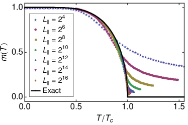
Figure 11: (Color online) Magnetization $m_{\mathrm{abs}}(T)$, Eq. (64a), of the $1\mathrm{d}$ system at $v=\infty$ for several system sizes $L_{\parallel}$ from Monte Carlo simulations, together with the exact solution Eq. (19).

The exact solution presented in Section III was derived in the thermodynamic limit $L_{\parallel}\to\infty$, as we assumed a constant and non-fluctuating order parameter $m$ in the self–consistence condition Eq. (15). This led to the result that the correlation length $\xi_{\parallel}$, Eq. (34), remains finite at criticality. However, in a finite system the assumption $m=\mathit{const}$ is not fulfilled and finite–size effects occur, leading to a non trivial dependency of the physical quantities on system size. The fluctuating order parameter gives rise to additional correlations between spins at large distances not included in the exact solution. As the driven system shows mean field behavior, we can use the standard finite–size scaling theory for mean field systems: Near criticality the correlation length parallel to the boundary fulfills $\xi_{\parallel}(\tau)\propto|\tau|^{-\nu_{\parallel}}$ with critical exponent $\nu_{\parallel}=2/d_{\mathrm{b}},$ where $d_{\mathrm{b}}$ denotes the boundary dimension. We have $d_{\mathrm{b}}=1$ in both the $1\mathrm{d}$ and the $2\mathrm{d}_{\mathrm{b}}$ case, leading to $\nu_{\parallel}=2$ in these cases.

To illustrate these finite–size effects in the $1\mathrm{d}$ case, in Fig. 11 we show the magnetization $m_{\mathrm{abs}}(T)$, Eq. (64a), as function of temperature for $v=\infty$ and several system sizes $L_{\parallel}$. The exact solution, Eq. (19), is only approached in the limit $L_{\parallel}\to\infty$.

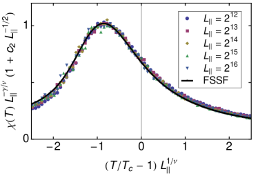
Figure 12: (Color online) Finite–size scaling plot of the reduced susceptibility $\chi_{\mathrm{abs}}(T)$, Eq. (64b), of the $1\mathrm{d}$ system for $v=\infty$ and system sizes $L_{\parallel}=2^{12},\ldots,2^{16}$, together with the exact mean field finite–size scaling function (black line) from Ref. (Grüneberg and Hucht, 2004). The correction factor $c_{2}=2.7$.

The finite–size scaling behavior is demonstrated exemplarily for the susceptibility $\chi_{\mathrm{abs}}(T)$, Eq. (64b), which is shown in a finite–size scaling plot in Fig. 12: After rescalation of the MC data in the usual way we indeed find the expected mean field exponents $\gamma=1$ and $\nu_{\parallel}=2$, furthermore the data falls onto the universal finite–size scaling function calculated in Ref. (Grüneberg and Hucht, 2004). The same analysis was performed for the magnetization $m_{\mathrm{abs}}(T)$ and specific heat $c(T)$, Eq. (64c), verifying the other two exponents $\beta=1/2$ and $\alpha=0$.

In summary, the $1\mathrm{d}$ and the $2\mathrm{d}_{\mathrm{b}}$ systems with boundary dimension $d_{\mathrm{b}}=1$ have the standard mean field exponents and fulfill the exponent relations

$$2-\alpha=2\beta+\gamma=d_{\mathrm{b}}\nu_{\parallel}.$$ (70)

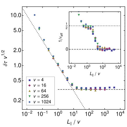
Figure 13: (Color online) Velocity dependent cross–over behavior in the $1\mathrm{d}$ case. Shown is the rescaled width of the critical region $\delta\tau\,v^{1/2}$ as function of the cross–over scaling variable $L_{\parallel}/v$ for several velocities $v$ and several system sizes $L_{\parallel}=2^{4},\ldots,2^{16}$ (see text). The inset shows the corresponding cross–over of the effective correlation length exponent $\nu_{\mathrm{eff}}^{-1}$ from $\nu_{\mathrm{eff}}^{-1}=1/2$ (MF, dotted line) to $\nu_{\mathrm{eff}}^{-1}=0$ (Ising non-critical, dashed line).

We now turn to finite velocities $v$: Then the $1\mathrm{d}$ system always shows a cross–over from mean field to Ising behavior with increasing system size $L_{\parallel}$. Only in the limit $v\rightarrow\infty$ the system undergoes a phase transition at finite temperatures. To investigate this velocity dependent cross–over, we measured the width $\delta\tau$ of the critical region by analysing the Binder cumulant Eq. (63c). Using least square fits of the simulation data to the simple approximation

$$U_{\mathrm{b}}(T)\approx\left\{\begin{array}[]{lll}{\displaystyle\frac{1}{3}[1+\tanh(\tilde{\tau}/\delta\tau)]}&&\tilde{\tau}\leq 0\\ \\ {\displaystyle\frac{1}{3}\frac{1}{1+\tilde{\tau}/\delta\tau}}&&\tilde{\tau}>0\end{array}\right.,$$ (71)

with $\tilde{\tau}=T/\tilde{T}_{\mathrm{c}}-1$ and fit parameters $\tilde{T}_{\mathrm{c}}$ and $\delta\tau$, for several velocities $v$ and system sizes $L_{\parallel}$ we determined $\delta\tau$ and plotted them in Fig. 13. We find that the cross–over scaling variable is $L_{\parallel}/v$ in this case, while the $y$-axis has to be rescaled as $\delta\tau\,v^{1/2}$ to get the correct limit $L_{\parallel}^{1/\nu_{\parallel}}\,\delta\tau=\mathit{const}$ with $\nu_{\parallel}=2$ in the limit $v\to\infty$. At finite $v$ the width $\delta\tau$ stops shrinking at $L_{\parallel}^{\times}\approx 9v$, where $L_{\parallel}^{\times}$ denotes the cross–over system size, and only goes to zero for $v\to\infty$, indicating a sharp phase transition in this limit. The inset shows the effective exponent $\nu_{\mathrm{eff}}$ obtained from the logarithmic derivative,

$$\nu_{\mathrm{eff}}^{-1}=-\frac{\partial\log\delta\tau}{\partial\log L_{\parallel}},$$ (72)

whose value changes from $\nu_{\mathrm{eff}}^{-1}=1/2$ (MF) to $\nu_{\mathrm{eff}}^{-1}=0$ (Ising) with growing system size. In the next section we will see that this behavior changes substantially in the $2\mathrm{d}_{\mathrm{b}}$ case.

IV.4 2d_b case

In the $2\mathrm{d}_{\mathrm{b}}$ case the moving boundary is coupled to a two-dimensional Ising model, which undergoes a phase transition at $T_{\mathrm{c,eq}}$, Eq. (4), independent of the velocity $v$. In addition, the moving boundary shows a boundary phase transition at temperature $T_{\mathrm{c}}(v)$, which grows with increasing $v$ and eventually approaches the value given in Eq. (50) for $v\to\infty$. As $T_{\mathrm{c}}(v)>T_{\mathrm{c,eq}}$ for all $v>0$ we expect a boundary phase transition with paramagnetic bulk. Then the correlation length $\xi_{\perp}$ perpendicular to the boundary is finite at criticality and has the Ising value

$$\xi_{\perp,\mathrm{c}}(v)=\xi_{\mathrm{eq}}(T_{\mathrm{c}}(v)),$$ (73)

with (McCoy and Wu, 1973)

$$\xi_{\mathrm{eq}}^{-1}(T)=\left\{\begin{array}[]{ll}4K-2\log\coth K&\qquad T<T_{\mathrm{c,eq}}\\ \log\coth K-2K&\qquad T>T_{\mathrm{c,eq}}\end{array}\right..$$ (74)

For that reason, in the finite–size scaling analysis it is sufficient for given $v$ to simulate systems with varying length $L_{\parallel}$ while holding the height $L_{\perp}$ fixed at a value $L_{\perp}\gg\xi_{\perp,\mathrm{c}}(v)$.

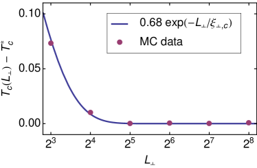
Figure 14: (Color online) Influence of the system size $L_{\perp}$ on the critical point in the $2\mathrm{d}_{\mathrm{b}}$ case at $v=\infty$ and $L_{\parallel}=256$. The effective critical temperature $T_{\mathrm{c}}(L_{\perp})$ shifts to higher values if $L_{\perp}\lesssim 10\xi_{\perp,\mathrm{c}}$ (see text).

To illustrate this behavior, in Fig. 14 we show the effect of different values of $L_{\perp}$ for $v=\infty$ and $L_{\parallel}=256$. Only below $L_{\perp}\approx 32$ the system feels the finite width $L_{\perp}$, resulting in a shift of the effective critical temperature $T_{\mathrm{c}}(L_{\perp})$ to higher values. The strength of the shift is proportional to the correlation function in $\perp$ direction, $\langle\sigma_{0,l}\sigma_{L_{\perp},l}\rangle\propto\exp(-L_{\perp}/\xi_{\perp,\mathrm{c}})$. The curves collapse for $L_{\perp}>32$ showing that a ratio $L_{\perp}/\xi_{\perp,\mathrm{c}}\approx 10$ is sufficient, as $\xi_{\perp,\mathrm{c}}(\infty)=3.66323\ldots$ in this case.

$v$	$T_{\mathrm{c}}^{*}(v)$	$T_{\mathrm{c}}^{\mathrm{M}}(v)$
$1/16$	$2.301(2)$
$1/4$	$2.33(1)\hphantom{0}$
$1$	$2.41(1)\hphantom{0}$	$2.30(2)$
$4$	$2.52(1)\hphantom{0}$	$2.37(2)$
$16$	$2.61(1)\hphantom{0}$	$2.42(2)$
$64$	$2.644(3)$	$2.44(2)$
$256$	$2.654(2)$	$2.44(2)$
$1024$	$2.659(2)$	$2.45(2)$
$\infty$	$2.661(1)$	$2.45(2)$

Table 1: Velocity dependent critical temperatures $T_{\mathrm{c}}(v)$ for the $2\mathrm{d}_{\mathrm{b}}$ case, estimated using the multiplicative rate, Eq. (69), with 400.000 MC sweeps per temperature as well as using the Metropolis rate, Eq. (66a), with 50.000 MC sweeps per temperature.

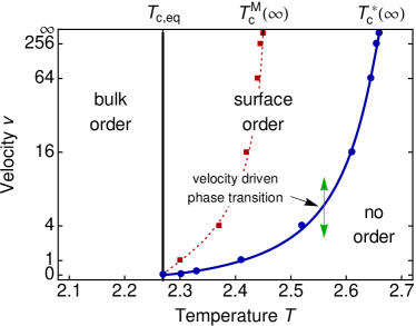
Figure 15: (Color online) Phase diagram of the $2\mathrm{d}_{\mathrm{b}}$ case. Below $T_{\mathrm{c,eq}}$ the two-dimensional bulk is ordered, while surface order is observed even above $T_{\mathrm{c,eq}}$ up to the velocity dependent phase boundary $T_{\mathrm{c}}(v)$. The position of this boundary depends on the algorithm, the blue line holds for the multiplicative rate, Eq. (69), while the thin red dotted line holds for the Metropolis rate, Eq. (66a). At fixed temperatures between $T_{\mathrm{c,eq}}$ and $T_{\mathrm{c}}(v)$ a velocity driven phase transition is possible. The points are results from MC simulations.

We performed MC simulations and determined the critical temperatures for different velocities $v$ by performing a finite–size scaling analysis of the boundary susceptibility $\chi_{\mathrm{abs,b}}(T)$ and the boundary cumulant $U_{\mathrm{b}}(T)$. For the multiplicative algorithm, Eq. (69), we used 400.000 MC steps per temperature, while for the Metropolis algorithm 50.000 MC steps per temperature were used. The results are given in Tab. 1 and are compiled into a phase diagram of the $2\mathrm{d}_{\mathrm{b}}$ case shown in Fig. 15. An important aspect of this phase diagram is the possibility of a velocity driven non–equilibrium phase transition at fixed temperature (double arrow): While the system is paramagnetic at $v=0$ and up to $v_{\mathrm{c}}(T)$ (thick blue line), the boundary shows long range order above that velocity. It would be interesting to see this transition in experiments, which could be performed in the corresponding geometry $3\mathrm{d}_{\mathrm{b}}$ (see Fig. 1), e.g., using two close rotating magnets slightly above the Curie temperature. The magnets should be isolating to avoid Eddy currents (Kadau et al., 2008).

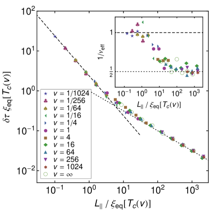
Figure 16: (Color online) Velocity dependent cross–over behavior in the $2\mathrm{d}_{\mathrm{b}}$ case. Shown is the rescaled width of the critical region $\delta\tau\,\xi_{\mathrm{eq}}[T_{\mathrm{c}}(v)]$ as function of the cross–over scaling variable $L_{\parallel}/\xi_{\mathrm{eq}}[T_{\mathrm{c}}(v)]$ for several velocities $v$ and different system sizes $L_{\parallel}=2^{4},\ldots,2^{10}$ (see text). The inset shows the corresponding cross–over of the effective correlation length exponent $\nu_{\mathrm{eff}}$ from $\nu_{\mathrm{eff}}=1$ (Ising, dashed line) to $\nu_{\mathrm{eff}}=2$ (MF, dotted line).

In the $2\mathrm{d}_{\mathrm{b}}$ case the cross–over scaling variable can be determined from the $T_{\mathrm{c}}(v)$ dependency discussed above. The correlation length $\xi_{\mathrm{eq}}$ at the critical point of the driven system, $T_{\mathrm{c}}(v)$, plays a key role: The system is Ising-like as long as correlations span the whole system in both directions $\parallel$ and $\perp$, i.e. as long as the system size $L_{\parallel}$ is of the order of the bulk correlation length $\xi_{\mathrm{eq}}$ at the critical point $T_{\mathrm{c}}(v)$ of the driven system, leading to the cross–over scaling variable $L_{\parallel}/\xi_{\mathrm{eq}}[T_{\mathrm{c}}(v)].$ Again, the rescaling of the $y$-axis can be determined by requiring that a data collapse is obtained in the limit $v\to 0$, leading to the expression $\delta\tau\,\xi_{\mathrm{eq}}[T_{\mathrm{c}}(v)]$, as $\xi_{\mathrm{eq}}$ cancels in this case and we get the required condition $L_{\parallel}\,\delta\tau=\mathit{const}$, as $\xi_{\mathrm{eq}}\propto\tau^{-\nu_{\mathrm{eq}}}$ in this limit, and $\nu_{\mathrm{eq}}=1$.

The resulting cross–over scaling plot is shown in Fig. 16. For all finite $v>0$ the critical behavior changes from Ising to mean field at the cross–over system size $L_{\parallel}^{\times}\approx 6\xi_{\mathrm{eq}}[T_{\mathrm{c}}(v)]$: Below this value $\delta\tau$ shrinks according to $\delta\tau\propto L_{\parallel}^{-1}$ (Ising, dashed line), while above this value $\delta\tau\propto L_{\parallel}^{-1/2}$ holds (MF, dotted line). As the shift exponent $\theta$ at small velocities, defined by

$$T_{\mathrm{c}}(v)-T_{\mathrm{c}}(0)\propto v^{\theta},$$ (75)

is close to $1/2$ we have, for small $v$, $L_{\parallel}^{\times}\propto v^{-\theta}\approx v^{-1/2}$. The shift exponent $\theta=1/2$ has also been found in a field theoretical calculation of the $2{+}1\mathrm{d}$ system (Gonnella and Pellicoro, 2000).

V Summary

In this work we investigated a recently proposed driven Ising model with friction due to magnetic correlations. The non–equilibrium phase transition present in this system was investigated in detail using analytical methods and Monte Carlo simulations. In the far from equilibrium limit of high driving velocities $v\to\infty$ the model was solved exactly by integrating out the non–equilibrium degrees of freedom. The resulting exact self–consistence equation was analysed for various geometries, leading in many cases to precise values of the critical temperature $T_{\mathrm{c}}$ of the non–equilibrium phase transition. In the limit $v\to\infty$ the system always shows mean field behavior due to dimensional reduction, independent of geometry. In the simplest one dimensional case denoted $1\mathrm{d}$ a complete analysis of both equilibrium as well as non–equilibrium quantities has been presented. These exact results are another example of mean field critical behavior in an exactly solvable driven system, just as in the case of the DLG in a certain limit (van Beijeren and Schulman, 1984).

The analytic results were reproduced using a multiplicative Monte Carlo rate originally introduced in (van Beijeren and Schulman, 1984), which eliminates correlations due to many particle dynamics introduced by the common Metropolis and Glauber rates. We claim that this algorithm is generally favorable to the Metropolis and Glauber rates if an analytical treatment is considered.

The finite–size effects naturally emerging in the simulations were analyzed using finite–size scaling techniques, a perfect agreement with exactly known universal finite–size scaling functions (Grüneberg and Hucht, 2004) were found.

We analysed the critical behavior at finite velocities and studied the cross–over behavior from low to high velocities: We found that the $1\mathrm{d}$ system only has a phase transition in the thermodynamic limit for $v=\infty$, while systems with finite $v$ always become non–critical at the cross–over system size $L_{\parallel}^{\times}\approx 9v$. On the contrary, the two–dimensional case $2\mathrm{d}_{\mathrm{b}}$ already has an Ising type phase transition at $v=0$, which changes to mean field behavior for all finite $v>0$ in the thermodynamic limit, at a cross–over length $L_{\parallel}^{\times}\approx 6\xi_{\mathrm{eq}}[T_{\mathrm{c}}(v)]$. In this sense, the velocity $v$ is a relevant perturbation, always driving the system to a non–equilibrium state.

The $1\mathrm{d}$ system changes from mean field to non–critical Ising universality, while the $2\mathrm{d}_{\mathrm{b}}$ case changes from Ising to mean field type with growing system size $L_{\parallel}$. This somewhat puzzling fact can be understood in terms of the critical width $\delta\tau$ of the transition as follows: As in general $\delta\tau\propto L_{\parallel}^{-1/\nu}$ at criticality, in the two dimensional Ising case $\delta\tau\propto L_{\parallel}^{-1}$, while in the mean field case with one dimensional boundary $\delta\tau\propto L_{\parallel}^{-1/2}$. Thirdly, $\delta\tau\propto L_{\parallel}^{0}=\mathit{const}$ in the $1\mathrm{d}$ case at finite $v$. In the cross–over the actual critical width $\delta\tau$ is always governed by the largest contribution, and so at sufficiently large system size $L_{\parallel}$ the contribution with smallest $\nu^{-1}$ dominates and determines the critical behavior. As consequence in both cases the effective inverse correlation length exponent $\nu_{\mathrm{eff}}^{-1}$ changes from a larger value at small $L_{\parallel}$ to a smaller value at large $L_{\parallel}$ ($1/2\to 0$ in the $1\mathrm{d}$ case, $1\to 1/2$ in the $2\mathrm{d}_{\mathrm{b}}$ case).

Comparing the results to the driven lattice gas (DLG) (Katz et al., 1983), we note that the DLG also shows a continuous non–equilibrium phase transition from an ordered to a disordered state at a critical temperature which grows with growing driving field. However, in the DLG the particle number is conserved, while we deal with a non-conserved magnetization.

Finally some remarks on strongly anisotropic critical behavior: The sheared system denoted $1{+}1\mathrm{d}$ shows strongly anisotropic behavior at criticality and $v\to\infty$, with strong evidence for the correlation length exponents $\nu_{\parallel}=3/2$ and $\nu_{\perp}=1/2$, details on this will be published elsewhere (Angst et al., 2010). Remarkably, this is a rare case of an exactly solvable non-equilibrium system with strongly anisotropic critical behavior.

Appendix A Surface magnetization of the $2d$ Ising model

The equilibrium surface magnetization $m_{\mathrm{b},\mathrm{eq}}$ of the $2d$ Ising model in a static surface field $h_{\mathrm{b}}$ obtained by McCoy and Wu (McCoy and Wu, 1973, Chapter VI, Eq. 5.1) as well as the reduced zero field boundary susceptibility

$$\chi_{\mathrm{b},\mathrm{eq}}^{(0)}=\left.\frac{\partial m_{\mathrm{b},\mathrm{eq}}}{\partial h_{\mathrm{b}}}\right|_{h_{\mathrm{b}}\rightarrow 0}$$ (76)

can be written in closed form not present in the literature yet (McCoy, 2008). $\chi_{\mathrm{b},\mathrm{eq}}^{(0)}$ is sometimes denoted $\chi_{11}$, and a high temperature series expansion was derived up to $10^{\mathrm{th}}$ order in Ref. (Binder and Hohenberg, 1972) and up to $23^{\mathrm{th}}$ order in Ref. (Enting and Guttmann, 1980). As the expressions for anisotropic couplings $K_{\parallel}$ and $K_{\perp}$ become way too complicated, we only give the results for the isotropic Ising model with $K_{\parallel}=K_{\perp}=K$ here: Using the definitions $z=\tanh K$, $y=\tanh h_{\mathrm{b}}$ we find

$$m_{\mathrm{b},\mathrm{eq}}(z,y) = \frac{z^{-1}-z}{\frac{z}{y}-\frac{y}{z}}\left[\frac{b^{2}}{2\pi}\mathop{\operator@font K}\nolimits(16w^{2})+\frac{b^{2}}{4\pi w}\frac{\bigl{(}a+\frac{y^{2}}{z}\bigr{)}^{2}}{1-\frac{by^{2}}{c^{2}z}}\mathop{\operator@font\Pi}\nolimits\!\left(\frac{\bigl{(}1-\frac{by^{2}}{z}\bigr{)}^{2}}{1-\frac{by^{2}}{c^{2}z}},16w^{2}\right)+\frac{Y^{1/2}-Y^{-1/2}}{2(z^{-1}-z)}-\frac{1}{4}\right],$$ (77)

$$\chi_{\mathrm{b},\mathrm{eq}}^{(0)}(z) = \left(\frac{1}{z^{2}}-1\right)\left[\left(1+2w-8w^{2}\right)\frac{\mathop{\operator@font K}\nolimits(16w^{2})}{4\pi w}-\frac{\mathop{\operator@font E}\nolimits(16w^{2})}{4\pi w}-\frac{1}{4}\right],$$ (78)

with the abbreviations

$$w = \frac{z(1-z^{2})}{(1+z^{2})^{2}}$$ (79a)

$$a = \frac{1-2z-z^{2}}{1+z^{2}}$$ (79b)

$$b = \frac{1+2z-z^{2}}{1+z^{2}}$$ (79c)

$$c = \frac{2z}{1+z^{2}}$$ (79d)

$$Y = \left(\frac{az}{c^{2}y^{2}}+1\right)\left(\frac{by^{2}}{c^{2}z}-1\right)^{-1}$$ (79e)

and the complete elliptic integrals of the $1^{\mathrm{st}}$, $2^{\mathrm{nd}}$ and $3^{\mathrm{rd}}$ kind, $\mathop{\operator@font K}\nolimits(m)$, $\mathop{\operator@font E}\nolimits(m)$ and $\mathop{\operator@font\Pi}\nolimits(n,m)$ Note that the variable $w$ is also used in high temperature series analysis of the bulk zero field susceptibility (Boukraa et al., 2008). For $h_{\mathrm{b}}=0$ the surface magnetization Eq. (77) reduces to the well known expression

$$m_{\mathrm{b},\mathrm{eq}}(K)=\sqrt{\frac{\cosh 2K-\coth 2K}{\cosh 2K-1}}.$$ (80)

References

• Fusco et al. (2008) C. Fusco, D. E. Wolf, and U. Nowak, Phys. Rev. B 77, 174426 (2008).
• Magiera et al. (2009a) M. P. Magiera, L. Brendel, D. E. Wolf, and U. Nowak, Europhys. Lett. 87, 26002 (6pp) (2009a).
• Magiera et al. (2009b) M. P. Magiera, D. E. Wolf, L. Brendel, and U. Nowak, IEEE Trans. Magn. 45, 3938 (2009b).
• Kadau et al. (2008) D. Kadau, A. Hucht, and D. E. Wolf, Phys. Rev. Lett. 101, 137205 (2008).
• Chan and Lin (1990) C. K. Chan and L. Lin, Europhys. Lett. 11, 13 (1990).
• Corberi et al. (1998) F. Corberi, G. Gonnella, and A. Lamura, Phys. Rev. Lett. 81, 3852 (1998).
• Cirillo et al. (2005) E. N. M. Cirillo, G. Gonnella, and G. P. Saracco, Phys. Rev. E 72, 026139 (2005).
• Imaeda and Kawasaki (1984) T. Imaeda and K. Kawasaki, Proc. Theor. Phys. 73, 559 (1984).
• Onuki (1997) A. Onuki, J. Phys: Condens. Matter 9, 6119 (1997).
• Katz et al. (1983) S. Katz, J. L. Lebowitz, and H. Spohn, Phys. Rev. B 28, 1655 (1983).
• Schmittmann and Zia (1995) B. Schmittmann and R. K. P. Zia, in Phase Transitions and Critical Phenomena, edited by C. Domb and J. L. Lebowitz (Academic Press, London, 1995), vol. 17.
• Stearns (1986) M. B. Stearns, in Magnetic Properties of Metals, edited by H. P. J. Wijn (Springer, Berlin, 1986), vol. III/19a of Landolt-Börnstein, New Series.
• Allen and Tildesley (1987) M. P. Allen and D. J. Tildesley, Computer Simulation of Liquids (Clarendon Press, Oxford, 1987).
• Onsager (1944) L. Onsager, Phys. Rev. 65, 117 (1944).
• Baxter (1982) R. J. Baxter, Exactly Solved Models in Statistical Mechanics (Academic Press, London, 1982).
• McCoy and Wu (1973) B. M. McCoy and T. T. Wu, The Two-Dimensional Ising Model (Harvard University Press, Cambridge, 1973).
• Ferrenberg and Landau (1991) A. M. Ferrenberg and D. P. Landau, Phys. Rev. B 44, 5081 (1991).
• Ito et al. (2000) N. Ito, K. Hukushima, K. Ogawa, and Y. Ozeki, J. Phys. Soc. Japan 69, 1931 (2000).
• Hucht (2002) A. Hucht, J. Phys A: Math. Gen. 35, L481 (2002).
• Angst et al. (2010) S. Angst, A. Hucht, and D. E. Wolf (2010), in preparation.
• Boukraa et al. (2008) S. Boukraa, A. J. Guttmann, S. Hassani, I. Jensen, J.-M. Maillard, B. Nickel, and N. Zenine, J. Phys A: Math. Gen. 41, 455202 (51pp) (2008), URL http://www.ms.unimelb.edu.au/~iwan/ising/Ising_ser.html.
• Binder and Hohenberg (1974) K. Binder and P. C. Hohenberg, Phys. Rev. B 9, 2194 (1974).
• Arisue and Fujiwara (2003) H. Arisue and T. Fujiwara, Nucl. Phys. B Proc. Suppl. 119, 855 (2003), arXiv:hep-lat/0209019, URL http://www.rccp.tsukuba.ac.jp/kenkyukai/asia-pacific/program/%transparency/arisue/asia-pacific2003b@.ps.
• Glauber (1963) R. J. Glauber, J. Math. Phys. 4, 294 (1963).
• Kawasaki (1965) K. Kawasaki, Phys. Rev. 145, 224 (1965).
• Metropolis et al. (1953) N. Metropolis, A. W. Rosenbluth, M. N. Rosenbluth, A. H. Teller, and E. Teller, J. Chem. Phys. 21, 1087 (1953).
• Kwak et al. (2004) W. Kwak, D. P. Landau, and B. Schmittmann, Phys. Rev. E 69, 066134 (2004).
• Grüneberg and Hucht (2004) D. Grüneberg and A. Hucht, Phys. Rev. E 69, 036104 (2004).
• Gonnella and Pellicoro (2000) G. Gonnella and M. Pellicoro, J. Phys A: Math. Gen. 33, 7043 (2000).
• van Beijeren and Schulman (1984) H. van Beijeren and L. S. Schulman, Phys. Rev. Lett. 53, 806 (1984).
• McCoy (2008) B. M. McCoy (2008), private communication.
• Binder and Hohenberg (1972) K. Binder and P. C. Hohenberg, Phys. Rev. B 6, 3461 (1972).
• Enting and Guttmann (1980) I. G. Enting and A. J. Guttmann, J. Phys A: Math. Gen. 13, 1043 (1980).
• Newman and Barkema (1999) M. E. J. Newman and G. T. Barkema, Monte Carlo Methods in Statistical Mechanics (Clarendon Press, Oxford, 1999).