The Effects of Gravitational Slip on the Higher-order Moments of the Matter Distribution

Abstract

Cosmological departures from general relativity offer a possible explanation for the cosmic acceleration. To linear order, these departures (quantified by the model-independent parameter $\varpi$, referred to as a ‘gravitational slip’) amplify or suppress the growth of structure in the universe relative to what we would expect to see from a general relativistic universe lately dominated by a cosmological constant. As structures collapse and become more dense, linear perturbation theory is an inadequate descriptor of their behavior, and one must extend calculations to non-linear order. If the effects of gravitational slip extend to these higher orders, we might expect to see a signature of $\varpi$ in the bispectrum of galaxies distributed on the sky. We solve the equations of motion for non-linear perturbations in the presence of gravitational slip and find that, while there is an effect on the bispectrum, it is too weak to be detected with present galaxy surveys. We also develop a formalism for incorporating scale dependence into our description of gravitational slip.

I Introduction

A universe in which gravity obeys the laws of general relativity and is filled with baryons and cold dark matter ought to decelerate. If we write the spatially-flat Robertson Walker metric

$$ds^{2}=a(\tau)^{2}[-d\tau^{2}+dr^{2}+r^{2}d\Omega^{2}].$$ (1)

deceleration means that $\dot{a}\equiv da/d\tau$ decreases with time. This is not the case in the Universe in which we live. Observations of distant supernovae indicate that our universe is, in fact, accelerating ($\dot{a}$ is growing with time) Riess:1998cb ; Perlmutter:1998np . To date, there are many theories vying to explain this acceleration. These theories can be generally divided into two categories: theories of dark energy and alternative theories of gravity. If we write Einstein’s equations as

$$R_{\mu\nu}-\frac{1}{2}g_{\mu\nu}R=8\pi GT_{\mu\nu},$$

dark energy attempts to explain the acceleration by modifying the right hand side (i.e., by positing that the universe is filled with an exotic new material). Alternative theories of gravity attempt to explain the acceleration by modifying the left hand side (i.e., by supposing that the laws of gravity obey different equations of motion on cosmological scales than they would under general relativity). Great diversity exists within both categories.

Dark energy can be Einstein’s cosmological constant Carroll:2000fy , a uniform energy density associated with the vacuum. Although this is the explanation currently favored by the data, there is no theoretical calculation justifying the observed value of the constant. Dark energy may also be a cosmological scalar field Zlatev:1998tr evolving slowly through its potential $V$ such that the equation of state $w\equiv\bar{p}/\bar{\rho}<0$ at late times. If this were the case, we would expect to see $w$ evolve with redshift at early times, which we do not. Dark energy could also be a vector field Jimenez:2008er , though these theories often introduce preferred reference frames or couplings between scalar and vector perturbation modes which we have yet to observe.

Alternative gravity can be a scalar-tensor theory Schimd:2004nq in which the dark energy scalar field is non-minimally coupled to the curvature terms in the Einstein-Hilbert action. These theories tend to predict departures from Newton’s law of gravitation, though the simplest of them merely manifest themselves as a rescaling of Newton’s constant $G$. There are also theories which modify gravity by introducing an arbitrary function of the Ricci scalar $f(R)$ into the gravitational Lagrangian Carroll:2004de ; Acquaviva:2004fv ; Zhang:2005vt . These theories tend to introduce new scale-dependent effects into the evolution of large scale structure. Tensor-vector-scalar (TeVeS) theory Bekenstein:2004ne ; Skordis:2005eu adds tensor and vector fields to the mix of scalar-tensor theory. These theories require precise couplings to avoid the pit-falls of vector dark energy noted above. Multi-dimensional braneworld theories (like the Dvali-Gabadadze-Porrati – DGP – model) Dvali:2000hr ; Lue:2005ya ; Song:2006jk attempt to account for cosmic acceleration by allowing gravity to act in dimensions outside of our $3+1$ Universe, imposing a scale beyond which the expected gravitational attraction is damped. Theories inspired by quantum mechanics, such as a Lorentz-violating massive graviton Bebronne:2007qh , reproduce solar system tests of gravity but introduce new classes of cosmological perturbations which may or may not show up in our measurements of large scale structure, depending on initial conditions.

All of these theories have solutions that can provide late-time cosmic acceleration. Successfully navigating this labyrinth of viable theories requires a set of observations complementary to the expansion of the universe for which different theories of gravity or dark energy predict different effects. The growth of cosmic structure provides one such set of observations. We model that growth using cosmic perturbation theory. If we consider only perturbations that transform like scalars, the first-order perturbed form of equation (1) is

$$ds^{2}=a^{2}[-(1+2\psi)d\tau^{2}+(1-2\phi)d\vec{x}^{2}].$$ (2)

Neglecting the cosmic scale factor $a$, the potentials $\psi$ and $\phi$ – known respectively as the Newtonian and longitudinal potentials – supply the right hand sides of Newton’s law of gravitation $\ddot{\vec{x}}=-\vec{\nabla}\psi$ and the Poisson equation $4\pi Ga^{2}\delta\rho=\nabla^{2}\phi$. Consistent with Newtonian dynamics, general relativity in the presence of non-relativistic stress-energy predicts that $\phi=\psi$. Alternative theories of gravity make no such guarantee. Each of the gravity theories cited above implies its own unique relationship between $\phi$ and $\psi$ Schimd:2004nq ; Acquaviva:2004fv ; Zhang:2005vt ; Skordis:2005eu ; Dvali:2000hr ; Lue:2005ya ; Song:2006jk ; Bebronne:2007qh .

Lacking theoretical justification to prefer one alternative gravity theory over another, we will content ourselves searching for evidence of gravitational slip (our word for the difference between $\phi$ and $\psi$) in general. Following Caldwell et al. Caldwell:2007cw , we parametrize the relationship between $\phi$ and $\psi$ as

$$\psi = (1+\varpi)\phi$$ (3)

$$\varpi = \varpi_{0}a^{3}.$$ (4)

Obviously, the scale independence and redshift dependence of equation (4) are assumptions on our part. Because we are interested in gravity theories which might explain the late time cosmic acceleration, we suppose that $\phi\approx\psi$ at high redshift and that gravitational slip should grow as the inverse of the matter density. For the purposes of our calculations, we will assume that the expansion history of the Universe exactly matches that of a $\Lambda$CDM universe, that is a universe which obeys general relativity ($\varpi$=0) and in which the acceleration is caused by a cosmological constant contributing a fraction $\Omega_{\Lambda}<1$ to the current density of the Universe.

Equation (3) is obviously not the only possible parametrization of modified gravity. References Bertschinger:2006aw ; Zhang:2007nk ; Hu:2007pj ; Amendola:2007rr ; Jain:2007yk ; Zhang:2008ba ; Bertschinger:2008zb ; Hu:2008zd all explore different model-independent expressions of $\phi\neq\psi$. Reference Daniel:2008et discusses the consistency of our choice (3) with these other parametrizations. In the end, it is simply a question of nomenclature.

References Daniel:2008et ; Daniel:2009kr , derived the linear-order equations of motion by perturbing a Robertson Walker metric (1) in the presence of a homogeneous, isotropic stress energy tensor

$$T^{\mu}_{\nu}=\text{diag}(-\bar{\rho},\bar{p},\bar{p},\bar{p})$$ (5)

and constrained $\varpi_{0}$ against CMB, supernova, and weak lensing (of galaxies) data sets. Specifically, reference Daniel:2009kr found the constraint $\varpi_{0}=0.09{}^{+0.74}_{-0.59}\,(2\sigma)$. Reference Serra:2009kp also tested equation (3), but against CMB and weak lensing (of the CMB) data sets. They also promoted the redshift dependence of equation (4) to a new free parameter. They found $\varpi_{0}=1.67^{+3.07}_{-1.87}\,(2\sigma)$. Both results are consistent with a $\Lambda$CDM universe obeying the laws of general relativity, but with significant room for departure ($\phi=\psi$ within a factor of a few). In this paper, we will attempt to complement those explorations by calculating the effect of non-zero $\varpi$ on the growth of structure in the Universe beyond linear order.

As gravitational collapse of structures progresses, the gravitational fields within overdense regions of the universe grow so that effects beyond linear order become important. Even in a $\varpi=0$ universe, this causes the distribution of overdensities to evolve away from their initial Gaussian distribution Peebles:1980 . These departures from Gaussianity are evidenced in the bispectrum, the Fourier transform of the three-point correlation function of galaxies. By altering the growth of structure Daniel:2009kr , $\varpi$ ought also to alter these departures from gaussianity, an effect which we hope will be detectable in modern galaxy surveys. Section II will derive the equations of motion for cosmic overdensities in the case of $\varpi\neq 0$ to “quasi-linear” order. Section III will translate these results into Fourier space. Section IV will calculate the resulting effects on the bispectrum. Section IV.1 includes the effects of galaxy bias and redshift distortions. Section V will consider the effect of adding scale dependence to $\varpi$. Section VI will discuss our results. Appendix A compares the results of our equations of motion (derived in Section II using Eulerian Perturbation Theory) to previous results derived in Lagrangian Perturbation Theory. Appendix B discusses the averaged second order moment of the overdensity distribution (the skewness). Appendix C extends our results to the next higher quasi-linear order, calculating the effect of scale-independent $\varpi$ on the kurtosis of the overdensity distribution.

II Equations of motion

This paper will work in the convention of Eulerian Perturbation Theory (see Appendix A for a discussion of Lagrangian Perturbation Theory). We will directly evolve the perturbed quantities $\phi$, $\delta\equiv(\rho-\bar{\rho})/\bar{\rho}$ and $\vec{v}$, the perturbed velocity field in the cold dark matter fluid. References Caldwell:2007cw ; Daniel:2008et ; Daniel:2009kr discuss how to modify the linear-order equations of motion for these perturbed quantities in the case of $\varpi\neq 0$. For the sake of brevity, we will merely summarize that discussion here. Of the linear-order perturbed Einstein equations presented in reference Ma:1995ey , the time-time and diagonal space-space are discarded. The time-space Einstein equation is preserved as a consequence of the assumption that the cold dark matter fluid remains, on average, at rest in our reference frame. A term is added to the off-diagonal space-space Einstein equation so to provide for $\varpi$ as a new source of cosmic shear. Because we have discarded the time-time and diagonal space-space Einstein equations, we can no longer assume that the Poisson equation is valid. This will be important when deriving the quasi-linear equations of motion below.

At quasi-linear order, gravitational collapse has advanced such that

$$\delta,v/c\gg\phi/c^{2},\psi/c^{2},$$ (6)

i.e. the dynamics of the local fluid dominate the dynamics of the spacetime. The metric is still Robertson Walker, but now, the stress energy tensor (5) is replaced by that of a perfect fluid

$$T^{\mu\nu}=(\bar{\rho}+\bar{p})u^{\mu}u^{\nu}+g^{\mu\nu}\bar{p}$$

where $u^{\mu}$ are the components of the fluid’s four-velocity Schutz:1985jx . To consistently determine the smallness of perturbed quantities, we explicitly include factors of $c$ in the perturbed metric (2), giving

$$\frac{ds^{2}}{c^{2}}=-a^{2}\left(1+2\frac{\psi}{c^{2}}\right)d\tau^{2}+\frac{a^{2}}{c^{2}}\left(1-2\frac{\phi}{c^{2}}\right)d\vec{x}^{2}$$ (7)

We derive our equations of motion by solving for the dynamics of this reformulated system to zeroth order in $1/c$. This is equivalent to assumption (6).

Requiring $u^{\mu}u_{\mu}=-1$, we find that

$$u^{\mu}=\gamma\left[\frac{1}{a}\left(1-\frac{\psi}{c^{2}}\right),\frac{\vec{v}}{a}\left(1+\frac{\phi}{c^{2}}\right)\right]$$ (8)

where $\gamma=1/\sqrt{1-\vec{v}^{2}/c^{2}}$, as usual. Thus, to the required order (because we are considering perturbations in the matter distribution, we set $\bar{p}=0$),

$$\nabla_{\mu}T^{\mu 0} = \frac{\gamma\bar{\rho}}{a^{2}}\left(\dot{\delta}+\partial_{i}(1+\delta)v^{i}\right)=0$$ (9)

$$\nabla_{\mu}T^{\mu i} = \frac{\gamma\bar{\rho}}{a^{2}}\left(\dot{v}^{i}+\mathcal{H}v^{i}+v^{j}\partial_{j}v^{i}+\partial_{i}\psi\right)=0$$ (10)

$$R_{0i} - \frac{1}{2}g_{0i}R=8\pi GT_{0i}$$ (11)

$$\phantom{\frac{1}{2}g_{0i}R}=\frac{1}{c^{2}}\left(2\partial_{0i}\phi+2\mathcal{H}\partial_{i}\psi\right)$$

$$\phantom{\frac{1}{2}g_{0i}R}=-8\pi Ga^{2}v^{i}\bar{\rho}(1+\delta)\frac{1}{c^{2}}$$

where $\mathcal{H}$ is the conformal time Hubble parameter $\mathcal{H}\equiv\dot{a}/a$. Note that, to lowest order, $\partial^{i}=a^{-2}\delta^{ij}\partial_{j}$. Equations (9) and (10) also correspond to equations (2) and (3) of Catelan and Moscardini’s paper deriving the quasi-linear fluid equations of motion in unmodified general relativity Catelan:1993zf . Their third equation of motion derives from the Poisson equation, which we discard in favor of our equation (11). (Note that Catelan and Moscardini use the coordinate time $t$ where we use the conformal time $\tau$). Following Catelan and Moscardini’s lead, we substitute equation (9) into the divergence of equation (10) to get

$$\ddot{\delta}+\mathcal{H}\dot{\delta} = (1+\varpi)\partial_{i}\delta\partial_{i}\phi$$

$$+\partial_{ij}[(1+\delta)v^{i}v^{j}]+(1+\delta)(1+\varpi)\nabla^{2}\phi$$

where we have used equation (3) to rewrite $\psi$ in terms of $\phi$ and $\varpi$. In our notation $\nabla^{2}\equiv\partial_{i}\partial_{i}$. Using equation (9), we can rewrite equation (11) as

$$\frac{3}{2}\mathcal{H}^{2}\Omega_{m}\dot{\delta}=\nabla^{2}\left(\dot{\phi}+\mathcal{H}(1+\varpi)\phi\right)$$ (13)

the time derivative of which is

$$\frac{3}{2}\Omega_{m}\mathcal{H}^{2}\left(\ddot{\delta}-\mathcal{H}\dot{\delta}\right) = \nabla^{2}\bigg{(}\ddot{\phi}+\mathcal{H}(1+\varpi)\dot{\phi}$$

$$+\mathcal{H}^{2}(1+\varpi)\phi(1-\frac{3}{2}\Omega_{m})+\mathcal{H}\dot{\varpi}\phi\bigg{)}.$$

Using equation (13), we find

$$\frac{3}{2}\Omega_{m}\mathcal{H}^{2}\left(\ddot{\delta}+\mathcal{H}\dot{\delta}\right) = \nabla^{2}\bigg{(}\ddot{\phi}+\mathcal{H}(3+\varpi)\dot{\phi}$$

$$+\mathcal{H}^{2}(1+\varpi)\phi(3-\frac{3}{2}\Omega_{m})+\mathcal{H}\dot{\varpi}\phi\bigg{)}.$$

Equations (II) and (II) provide an algorithm by which we can solve for $\phi$ and $\delta$ to arbitrary order. Once we have solved for $\phi$ and $\delta$, it is a simple matter to use equation (9) to find $\vec{v}$.

Assume that $\phi$, $\delta$ and $\vec{v}$ can be expanded as $\phi=\sum_{i}\phi^{(i)}$ etc., where $\phi^{(i)}\gg\phi^{(j>i)}$ (i.e., “$\phi^{(i)}$ is the $i$th order part of $\phi$”). In that case, we can expand equations (II) and (II) to a given order $n$, then use the proportionality between their left hand sides to get a single equation of the form

$$\nabla^{2}\Bigg{(}\ddot{\phi}^{(n)} + \dot{\phi}^{(n)}\mathcal{H}(3+\varpi)+\phi^{(n)}\left[\mathcal{H}^{2}3(1+\varpi)(1-\Omega_{m})+\mathcal{H}\dot{\varpi}\right]\Bigg{)}=\frac{3}{2}\Omega_{m}\mathcal{H}^{2}S^{(n)}$$ (15)

$$S^{(n)} \equiv \sum_{a+b+c=n}\Big{\{}(1+\varpi)\partial_{i}\delta^{(a)}\partial_{i}\phi^{(b)}+\partial_{ij}[(1+\delta^{(a)})v^{(b)i}v^{(c)j}]+\delta^{(a)}(1+\varpi)\nabla^{2}\phi^{(b)}\Big{\}}$$ (16)

where the source terms $S^{(n)}$ come from the non-linear part of equation (II). After solving equation (15) for $\nabla^{2}\phi^{(n)}$, one can use equation (II)

$$\ddot{\delta}^{(n)}+\mathcal{H}\dot{\delta}^{(n)}=S^{(n)}+(1+\varpi)\nabla^{2}\phi^{(n)}$$ (17)

to solve for $\delta^{(n)}$.

Comparing equations (15) and (17), we see that, even though the Poisson equation no longer holds, $\phi$ and $\delta$ are still separable at first order ($\phi=f(\tau)\varphi(\vec{x})$ and $\delta=D(\tau)\xi(\vec{x})$) and related such that the spatial parts of $\delta$ are the Laplacians of the spatial parts of $\phi$ (i.e., $\xi=\nabla^{2}\varphi$). Indeed, to first order

$$\phi^{(1)} = f(\tau)\varphi(\vec{x})$$ (18)

$$\delta^{(1)} = D(\tau)\nabla^{2}\varphi(\vec{x})$$ (19)

$$\vec{v}^{(1)} = -\dot{D}\vec{\nabla}\varphi$$ (20)

$$\dot{f}+f\mathcal{H}(1+\varpi) = \frac{3}{2}\Omega_{m}\mathcal{H}^{2}\dot{D}$$

$$\ddot{D}+\mathcal{H}\dot{D} = (1+\varpi)f.$$

At higher orders, the expressions are less compact

$$\phi^{(2)} = \alpha(\tau)A(\vec{x})+\beta(\tau)B(\vec{x})$$

$$\delta^{(2)} = \mathcal{D}^{a}\nabla^{2}A+\mathcal{D}^{b}\nabla^{2}B$$ (21)

$$\vec{v}^{(2)} = \vec{\nabla}A(-\dot{\mathcal{D}}^{a}+D\dot{D})-\vec{\nabla}B\dot{\mathcal{D}}^{b},$$ (22)

where

$$\nabla^{2}A = \partial_{i}\left(\nabla^{2}\varphi\partial_{i}\varphi\right)$$ (23)

$$\nabla^{2}B = \partial_{ij}\left(\partial_{i}\varphi\partial_{j}\varphi\right)$$ (24)

$$\ddot{\alpha} = -\dot{\alpha}\mathcal{H}(3+\varpi)+\frac{3}{2}\Omega_{m}\mathcal{H}^{2}(1+\varpi)Df-\alpha\left[3\mathcal{H}^{2}(1+\varpi)(1-\Omega_{m})+\dot{\varpi}\mathcal{H}\right]$$ (25)

$$\ddot{\beta} = -\dot{\beta}\mathcal{H}(3+\varpi)+\frac{3}{2}\Omega_{m}\mathcal{H}^{2}\dot{D}^{2}-\beta\left[3\mathcal{H}^{2}(1+\varpi)(1-\Omega_{m})+\dot{\varpi}\mathcal{H}\right]$$ (26)

$$\ddot{\mathcal{D}}^{a} = -\mathcal{H\dot{D}}^{a}+(1+\varpi)\alpha+(1+\varpi)Df$$ (27)

$$\ddot{\mathcal{D}}^{b} = -\mathcal{H\dot{D}}^{b}+(1+\varpi)\beta+\dot{D}^{2}.$$ (28)

In the $\varpi=0$ limit, these expressions agree with the GR results of Kamionkowski:1998fv . There are seven different spatial functions comprising $\phi^{(3)}$. We present them in Appendix C.1.

We now only lack initial conditions on the relevant growth terms in our attempt to solve for $\delta$ in the quasi-linear regime. Since the power spectrum $P_{\delta}$ is initially Gaussian, non-linear growth terms (i.e., $\alpha$ and $\beta$ from equation (21)) are integrated from the early-time initial conditions $\alpha_{i}=0$, $\dot{\alpha}_{i}=0$. To find the initial conditions for the linear growth terms $f$ and $D$, we combine the first order equations of motion (II) and (13), giving

$$\ddot{D}+\dot{D}\mathcal{H} = (1+\varpi)f$$

$$\dot{f}+f\mathcal{H}(1+\varpi) = \frac{3}{2}\Omega_{m}\mathcal{H}^{2}\dot{D}$$

to get

$$\dot{f} = \frac{3}{2}\Omega_{m}\mathcal{H}^{2}\dot{D}-\mathcal{H}^{2}\dot{D}-\mathcal{H}\ddot{D}$$

$$= -\dot{\mathcal{H}}\dot{D}-\mathcal{H}\ddot{D}$$

$$= -\frac{d}{d\tau}\left(\mathcal{H}\dot{D}\right)$$

$$f = -\mathcal{H}\dot{D}+C$$ (29)

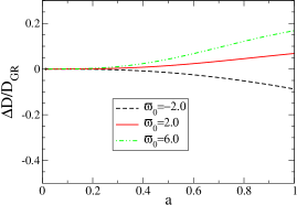
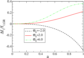
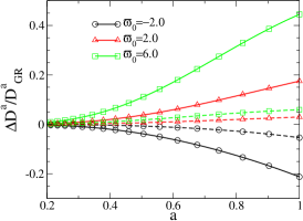
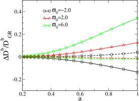
where $C$ is a constant. Since we assume that $\lim_{a\rightarrow 0}\varpi=0$, we use the $\Lambda$CDM equations of motion combined with the Poisson-equation result $f=(3/2)\Omega_{m}\mathcal{H}^{2}D$ to find the correct value for $C$ for a given $\Omega_{m}$. This value changes depending on the initial conditions assumed for $D$ and $\dot{D}$. However, the normalization of the measured statistic (56) means that our final results are resilient to such choices. Figure 1 plots the effect of gravitational slip on the first order growth function $D$ and its derivative. Figure 2 plots the same effects on the second order growth functions $\mathcal{D}^{a}$ and $\mathcal{D}^{b}$.

Figure 1: We plot the change in the first order growth functions $D$ and $f_{1}\equiv\frac{a}{D}\frac{dD}{da}$ resulting from varying $\varpi_{0}$. Note that $f_{1}$ is a different parameter from the $f$ used in equation (18). All other parameters are set to be the WMAP 5-year maximum likelihood values Dunkley:2008ie . The change is calculated relative to a $\varpi=0$ (GR) model so that $\Delta D/D_{GR}=(D-D_{GR})/D_{GR}$. As found in Daniel:2008et , $\varpi_{0}>0$ amplifies the growth of $\delta^{(1)}$, while $\varpi_{0}<0$ suppresses it.

Figure 2: We plot the change in the second order growth functions $\mathcal{D}^{a}$ and $\mathcal{D}^{b}$ resulting from varying $\varpi_{0}$. All other parameters are set to be the WMAP 5-year maximum likelihood values Dunkley:2008ie . In the case of solid lines, $\Delta\mathcal{D}^{i}\equiv\mathcal{D}^{i}-\mathcal{D}^{i}_{GR}$. In the case of dashed lines, the second order growth functions are normalized by a factor of $D^{2}$ ($D$ is the first order growth function) so that $\Delta\mathcal{D}^{i}\equiv\mathcal{D}^{i}(D_{GR}/D)^{2}-\mathcal{D}^{i}_{GR}$. The normalization greatly diminishes the effect of varying $\varpi_{0}$, indicating that most of the effect of $\varpi_{0}$ on the higher order growth functions enters as a normalization.

III Fourier transform of $\langle\delta^{n}\rangle$

In Section IV we will derive an expression for the bispectrum of the matter distribution in the case of $\varpi\neq 0$. This calculation will require taking the Fourier transform of terms like $\langle\delta^{n}(\vec{x})\rangle$ for $n>1$, which we illustrate below.

If we expand $\delta(\vec{x})=\sum_{i}\delta^{(i)}(\vec{x})$, then

$$\langle\delta^{n}\rangle = \langle(\delta^{(1)})^{n}\rangle+n\langle\delta^{(2)}(\delta^{(1)})^{n-1}\rangle+n\langle\delta^{(3)}(\delta^{(1)})^{n-1}\rangle+\binom{n}{2}\langle(\delta^{(2)})^{2}(\delta^{(1)})^{n-2}\rangle+\dots$$ (30)

(note: superscripts in parentheses are orders of expansion; superscripts outside parentheses are exponents). Therefore, in order to get the Fourier tranform of $\langle\delta^{n}\rangle$, we first need the Fourier transform of $\langle\delta^{(i)}\rangle$. From the form of equation (17), we can see that

$$\delta^{(i)}(\vec{x})=D^{(i)}(\tau)\Delta(\varphi_{1},\varphi_{2},\dots,\varphi_{i})$$ (31)

where $D^{(i)}$ stands for some combination of $i$th order growth functions and $\Delta$ is some combination of spatial derivatives acting on the $i$ powers of $\varphi(\vec{x})$ (see, for example, equation 21). Taking the Fourier transform of this qualitative $\delta^{(i)}$, we find (here we will introduce the notation $\tilde{\delta}^{(i)}_{a}\equiv\tilde{\delta}^{(i)}(\vec{k}_{a})$)

$$\tilde{\delta}^{(i)}(\vec{k})=\int\frac{d^{3}x}{(2\pi)^{3/2}}e^{-i\vec{k}\vec{x}}D^{(i)}\Delta(\varphi_{1},\dots,\varphi_{i})$$ (32)

$$=\int\frac{d^{3}xd^{3}k_{1\dots i}}{(2\pi)^{\frac{3}{2}(i+1)}}e^{i\vec{x}(\sum_{j=1}^{i}\vec{k}_{j}-\vec{k})}D^{(i)}\mathcal{K}\prod_{m=1}^{i}\tilde{\varphi}_{m}$$ (33)

$$=\int\frac{d^{3}k_{1\dots i}}{(2\pi)^{\frac{3}{2}(i-1)}}\delta^{3}_{D}(\vec{k}-\sum_{j=1}^{i}\vec{k}_{j})D^{(i)}\mathcal{K}\prod_{m=1}^{i}\tilde{\varphi}_{m}$$ (34)

$$=\int\frac{d^{3}k_{1\dots i}}{(2\pi)^{\frac{3}{2}(i-1)}}\delta^{3}_{D}(\vec{k}-\sum_{j=1}^{i}\vec{k}_{j})\times\frac{(-1)^{i}D^{(i)}\mathcal{K}}{(D^{(1)})^{i}}\prod_{{l}=1}^{i}\frac{\tilde{\delta}^{(1)}_{l}}{k^{2}_{l}}$$ (35)

(note $d^{3}k_{1\dots i}\equiv\prod_{j=1}^{i}d^{3}k_{j}$) where, in going from equation (32) to (33), we have taken the Fourier transform of each individual factor of $\varphi(\vec{x})$ in equation (31). $\mathcal{K}$ represents the combination of wave vectors $\{\vec{k}_{1},\vec{k}_{2},\dots\vec{k}_{i}\}$ deriving from the differential operator $\Delta$. $\delta^{3}_{D}$ is a Dirac delta function. We used equation (19) to go from equation (34) to (35).

From equation (35), we can see that a term of the form $\delta^{(i)}(\vec{x})(\delta^{(1)}(\vec{x}))^{n}$ can be written in terms of Fourier transforms as

$$\delta^{(i)}(\vec{x})(\delta^{(1)}(\vec{x}))^{n} = \int\frac{d^{3}kd^{3}k_{1\dots n}}{(2\pi)^{\frac{3}{2}(n+1)}}e^{i\vec{x}(\vec{k}+\sum_{j=1}^{n}\vec{k}_{j})}\times\tilde{\delta}^{(i)}\prod_{m=1}^{n}\tilde{\delta}^{(1)}_{m}$$ (36)

$$= \int\frac{d^{3}kd^{3}k_{1\dots n}}{(2\pi)^{\frac{3}{2}(n+1)}}\frac{d^{3}k^{\prime}_{1\dots i}}{(2\pi)^{\frac{3}{2}(i-1)}}e^{i\vec{x}(\vec{k}+\sum_{j=1}^{n}\vec{k}_{j})}\prod_{m=1}^{n}\tilde{\delta}^{(1)}_{m}\times\delta^{3}_{D}(\vec{k}-\sum_{l=1}^{i}\vec{k}^{\prime}_{l})\frac{(-1)^{i}D^{(i)}}{(D^{(1)})^{i}}\mathcal{K}\prod_{b=1}^{i}\frac{\tilde{\delta}^{(1)\prime}_{b}}{k^{\prime 2}_{b}}$$

where, to be explicit, the $k^{\prime}_{j}$ wave vectors come from the Fourier transform $\tilde{\delta}^{(i)}$. Integrating the right hand side of equation (36) over the wave vector $\vec{k}$, we see that

$$\delta^{(i)}(\vec{x})(\delta^{(1)})^{n} = \int\frac{d^{3}k_{1\dots i+n}}{(2\pi)^{\frac{3}{2}(i+n)}}e^{i\vec{x}\cdot(\sum_{j=1}^{i+n}\vec{k}_{j})}\times\frac{D^{(i)}}{(D^{(1)})^{i}}\frac{\mathcal{K}}{\prod_{l=1}^{i}k^{2}_{l}}\prod_{j=1}^{i+n}\tilde{\delta}^{(1)}_{j}$$

whence

$$\langle\delta^{(i)}(\vec{x})(\delta^{(1)})^{n}\rangle = \int\frac{d^{3}k_{1\dots i+n}}{(2\pi)^{\frac{3}{2}(i+n)}}e^{i\vec{x}\cdot(\sum_{j=1}^{i+n}\vec{k}_{j})}\times\frac{(-1)^{i}D^{(i)}}{(D^{(1)})^{i}}\frac{\mathcal{K}}{\prod_{l=1}^{i}k^{2}_{l}}\times\langle\tilde{\delta}^{(1)}_{1}\dots\tilde{\delta}^{(1)}_{i+n}\rangle.$$ (37)

At this point, it is useful to recall that, for a Gaussian field (like $\tilde{\delta}^{(1)})$,

$$\langle\tilde{\delta}^{(1)}_{1}\tilde{\delta}^{(1)}_{2}\dots\tilde{\delta}^{(1)}_{n}\rangle = 0\phantom{\langle\delta^{1}\delta\delta\dots\delta\dots 2+\text{permutations}}\qquad\text{$n$ odd}$$ (39)

$$= \langle\tilde{\delta}^{(1)}_{1}\tilde{\delta}^{(1)}_{2}\rangle\langle\tilde{\delta}^{(1)}_{3}\tilde{\delta}^{(1)}_{4}\rangle\dots\langle\tilde{\delta}^{(1)}_{n-1}\tilde{\delta}^{(1)}_{n}\rangle$$

$$\phantom{\langle\delta^{1}\delta\delta\dots\delta\dots 2}+\phantom{2}\text{permutations}\qquad\text{$n$ even}$$

so that, for example

$$\langle\tilde{\delta}^{(1)}_{1}\tilde{\delta}^{(1)}_{2}\tilde{\delta}^{(1)}_{3}\rangle = 0$$

$$\langle\tilde{\delta}^{(1)}_{1}\tilde{\delta}^{(1)}_{2}\tilde{\delta}^{(1)}_{3}\tilde{\delta}^{(1)}_{4}\rangle = \phantom{+}\langle\tilde{\delta}^{(1)}_{1}\tilde{\delta}^{(1)}_{2}\rangle\langle\tilde{\delta}^{(1)}_{3}\tilde{\delta}^{(1)}_{4}\rangle$$

$$+\langle\tilde{\delta}^{(1)}_{1}\tilde{\delta}^{(1)}_{3}\rangle\langle\tilde{\delta}^{(1)}_{2}\tilde{\delta}^{(1)}_{4}\rangle$$

$$+\langle\tilde{\delta}^{(1)}_{1}\tilde{\delta}^{(1)}_{4}\rangle\langle\tilde{\delta}^{(1)}_{3}\tilde{\delta}^{(1)}_{2}\rangle.$$

From this, we see that the right hand side of equation (37) involves $(i+n-1)(i+n-3)\dots(1)$ terms if $(i+n)$ is even. If $(i+n)$ is odd, equation (37) is identically zero. Finally, we recall that

$$\langle\tilde{\delta}^{(1)}_{1}\tilde{\delta}^{(1)}_{2}\rangle=\delta^{3}_{D}(\vec{k}_{1}+\vec{k}_{2})P_{\delta}(k_{1})$$ (40)

Combining these results with equation (30) gives us an algorithm for evaluating the higher order correlation functions of the $\delta$ distribution. We illustrate this by considering the bispectrum.

IV The bispectrum

The bispectrum is the three point equivalent of the power spectrum, i.e. it is the Fourier transform of the three-point correlation function. In the expression

$$\langle\delta(\vec{x}_{1})\delta(\vec{x}_{2})\delta(\vec{x}_{3})\rangle = \langle\int\frac{d^{3}k_{1\dots 3}}{(2\pi)^{9/2}}e^{i\sum_{j=1}^{3}\vec{x}_{j}\vec{k}_{j}}\prod_{l=1}^{3}\tilde{\delta}(\vec{k}_{l})\rangle$$

$$= \int\frac{d^{3}k_{1\dots 3}}{(2\pi)^{9/2}}e^{i\sum_{j=1}^{3}\vec{x}_{j}\vec{k}_{j}}\mathcal{B}(\vec{k}_{1},\vec{k}_{2},\vec{k}_{3})$$

$\mathcal{B}$ is the bispectrum. From equations (30) and (39), we see that the three-point correlation function will, to leading order, be made up of three terms like

$$\langle\delta^{(2)}\delta^{(1)}\delta^{(1)}\rangle.$$

We write $\delta^{(2)}$, using equations (21), (23) and (24), as

$$\delta^{(2)} = \mathcal{D}^{a}\Big{(}\partial_{i}\varphi\partial_{i}\nabla^{2}\varphi+\nabla^{2}\varphi\nabla^{2}\varphi\Big{)}+\mathcal{D}^{b}\Big{(}\partial_{ij}\varphi\partial_{ij}\varphi+\nabla^{2}\varphi\nabla^{2}\varphi+2\partial_{i}\varphi\partial_{i}\nabla^{2}\varphi\Big{)}.$$

From equation (35), we see that this means

$$\tilde{\delta}^{(2)}(\vec{k}) = \int d^{3}k^{\prime}d^{3}k^{\prime\prime}\frac{\tilde{\delta}(\vec{k}^{\prime})\tilde{\delta}(\vec{k}^{\prime\prime})}{D^{2}}\delta^{3}_{D}(\vec{k}-\vec{k}^{\prime}-\vec{k}^{\prime\prime})\times\Big{[}\mathcal{D}^{a}\Big{(}1+\frac{\vec{k}^{\prime}\cdot\vec{k}^{\prime\prime}}{k^{\prime 2}}\Big{)}+\mathcal{D}^{b}\Big{(}1+2\frac{\vec{k}^{\prime}\cdot\vec{k}^{\prime\prime}}{k^{\prime 2}}+\frac{(\vec{k}^{\prime}\cdot\vec{k}^{\prime\prime})^{2}}{k^{\prime 2}k^{\prime\prime 2}}\Big{)}\Big{]}$$ (41)

$$= \int\frac{d^{3}k^{\prime}}{(2\pi)^{3/2}}\frac{\tilde{\delta}(\vec{k}^{\prime})\tilde{\delta}(\vec{k}-\vec{k}^{\prime})}{D^{2}}\Big{[}\mathcal{D}^{a}\Big{(}1+\frac{\vec{k}^{\prime}\cdot(\vec{k}-\vec{k}^{\prime})}{k^{\prime 2}}\Big{)}+\mathcal{D}^{b}\Big{(}1+2\frac{\vec{k}^{\prime}\cdot(\vec{k}-\vec{k}^{\prime})}{k^{\prime 2}}+\frac{(\vec{k}^{\prime}\cdot(\vec{k}-\vec{k}^{\prime}))^{2}}{k^{\prime 2}(\vec{k}-\vec{k}^{\prime})^{2}}\Big{)}\Big{]}$$

We can now average equation (41) with two factors of $\tilde{\delta}(\vec{k})$ to find the form of the bispectrum.

$$\langle\tilde{\delta}^{(1)}_{1}\tilde{\delta}^{(1)}_{2}\tilde{\delta}^{(2)}_{3}\rangle = \int\frac{d^{3}k_{4}}{D^{2}}\langle\tilde{\delta}^{(1)}_{1}\tilde{\delta}^{(1)}_{2}\tilde{\delta}^{(1)}_{3-4}\tilde{\delta}^{(1)}_{4}\rangle\times\Big{[}\mathcal{D}^{a}\Big{(}1+\frac{\vec{k}_{4}\cdot(\vec{k}_{3}-\vec{k}_{4})}{k_{4}^{2}}\Big{)}+\mathcal{D}^{b}\Big{(}1+2\frac{\vec{k}_{4}\cdot(\vec{k}_{3}-\vec{k}_{4})}{k_{4}^{2}}+\frac{(\vec{k}_{4}\cdot(\vec{k}_{3}-\vec{k}_{4}))^{2}}{k_{4}^{2}(\vec{k_{3}}-\vec{k}_{4})^{2}}\Big{)}\Big{]}$$ (42)

$$= \int\frac{d^{3}k_{4}}{D^{2}}\Big{\{}P(k_{1})P(k_{2})\delta^{3}_{D(1+3-4)}\delta^{3}_{D(2+4)}+P(k_{1})P(k_{2})\delta^{3}_{D(1+4)}\delta^{3}_{D(2+3-4)}+P(k_{1})P(k_{4})\delta^{3}_{D(1+2)}\delta^{3}_{D(3)}\Big{\}}$$

$$\times\Big{[}\mathcal{D}^{a}\Big{(}1+\frac{\vec{k}_{4}\cdot(\vec{k}_{3}-\vec{k}_{4})}{k_{4}^{2}}\Big{)}+\mathcal{D}^{b}\Big{(}1+2\frac{\vec{k}_{4}\cdot(\vec{k}_{3}-\vec{k}_{4})}{k_{4}^{2}}+\frac{(\vec{k}_{4}\cdot(\vec{k}_{3}-\vec{k}_{4}))^{2}}{k_{4}^{2}(\vec{k_{3}}-\vec{k}_{4})^{2}}\Big{)}\Big{]}$$

(note $\delta^{3}_{D(i+j-l)}\equiv\delta^{3}_{D}(\vec{k}_{i}+\vec{k}_{j}-\vec{k}_{l})$) where we have used equation (40) to get the power spectra and $\delta^{3}_{D}$ factors. Note that, by the coefficients of the growth terms, the $\delta^{3}_{D}(\vec{k}_{3})$ term will vanish upon integration. Once that term is discarded, we see that the bispectrum is proportional to $\delta^{3}_{D}(\vec{k}_{1}+\vec{k}_{2}+\vec{k}_{3})$. Specifically

$$\mathcal{B}(\vec{k}_{1},\vec{k}_{2},\vec{k}_{3}) = \frac{P(k_{1})P(k_{2})}{D^{2}}\Big{[}\mathcal{D}^{a}(1+\frac{\vec{k}_{2}\cdot\vec{k}_{1}}{k_{2}^{2}})+\mathcal{D}^{b}(1+2\frac{\vec{k}_{2}\cdot\vec{k_{1}}}{k_{2}^{2}}+\frac{(\vec{k}_{2}\cdot\vec{k}_{1})^{2}}{k_{2}^{2}k_{1}^{2}}\Big{]}\delta^{3}_{D}(\vec{k}_{1}+\vec{k}_{2}+\vec{k}_{3})$$ (43)

$$+\frac{P(k_{1})P(k_{2})}{D^{2}}\Big{[}\mathcal{D}^{a}(1+\frac{\vec{k}_{2}\cdot\vec{k}_{1}}{k_{1}^{2}})+\mathcal{D}^{b}(1+2\frac{\vec{k}_{2}\cdot\vec{k_{1}}}{k_{1}^{2}}+\frac{(\vec{k}_{2}\cdot\vec{k}_{1})^{2}}{k_{2}^{2}k_{1}^{2}}\Big{]}\delta^{3}_{D}(\vec{k}_{1}+\vec{k}_{2}+\vec{k}_{3})$$

$$+\text{permutations}.$$

It is straightforward to integrate the equations in Section II and determine how $\varpi_{0}$ affects equation (43). It is less straightforward to turn this calculation into a real-world constraint on $\varpi_{0}$.

IV.1 Galaxy bias and redshift distortions

It is presently impossible to measure the dark matter density at all points in space. As its name suggests, we cannot see dark matter. We can only see the galaxies that form in dark matter haloes. Going from astronomical observations to a determination of the bispectrum (43) requires assumptions about how the galaxy distribution tracks the dark matter distribution (the “galaxy bias”) for which we have little theoretical motivation. As if that were not hard enough, we only actually see the galaxies in two dimensions (altitude and azimuth relative to our telescope). We infer the radial distance to galaxies by measuring their redshift and assuming that Hubble’s law is valid. This is a decent assumption for redshifts of a few. Unfortunately, it means that galactic peculiar motions interfere with our determination of galaxies’ positions, giving rise to “redshift distortions” in the observed distribution of galaxies. It is known how to correct for these effects in calculating equation (43). We will do so below. Our derivation relies heavily on the $\varpi=0$ calculations presented by Bernardeau in Section 7 of reference Bernardeau:2001qr .

The correction for scale- and time-independent galaxy bias is simple. Assume that the excess number density of galaxies $\delta_{g}=(n_{g}-\bar{n}_{g})/\bar{n}_{g}$ relates to the matter overdensity $\delta$ by

$$\delta_{g}=\sum_{i}\frac{b_{i}\delta^{i}}{i!}$$

where $b_{i}$ are (constant) coefficients of the expansion. If we then write the overdensity $\delta$ as we did in the discussion leading up to equation (30), we have, to second order

$$\delta_{g}=b_{1}\delta^{(1)}+b_{1}\delta^{(2)}+\frac{b_{2}}{2}(\delta^{(1)})^{2}+\dots$$ (44)

To first order, the expansion is simply $\delta_{g}=b_{1}\delta$.

To account for redshift space distortions, we follow Section 7 of reference Bernardeau:2001qr or Section 9.4 of reference Dodelson:2003ft . We denote redshift space (in which radial distance is reckoned from Hubble’s law) by $\vec{x}_{s}$. Physical space will remain $\vec{x}$. Because observations are made in redshift space, we want to calculate the bispectrum of the redshift space distribution using the physical space evolution equations we derived in Section II. We will work in the plane-parallel approximation in which the sky is flat and the radial direction is $\hat{z}$. By Hubble’s law, the redshift space $z$ coordinate of a given galaxy will be

$$z_{s}=z_{x}+\frac{v_{z}}{\mathcal{H}_{0}}.$$ (45)

We use the conformal time Hubble parameter because, throughout this work, $\vec{v}$ has also been calculated as the conformal time velocity. It is also true that $\mathcal{H}_{0}=H_{0}$ as long as $a_{0}=1$. From equation (45), we have

$$\frac{d^{3}x_{s}}{d^{3}x}=\frac{dx_{s}dy_{s}dz_{s}}{dxdydz}=1+\frac{1}{\mathcal{H}_{0}}\partial_{z}v_{z}.$$

Because we do not want our change in coordinates to change the mass of a given region, we set

$$(1+\delta_{s})d^{3}x_{s}=(1+\delta)d^{3}x$$ (46)

from which we find

$$\delta_{s} = (1+\delta)\frac{d^{3}x}{d^{3}x_{s}}-1$$

$$= \left(1+\delta-\frac{d^{3}x_{s}}{d^{3}x}\right)\frac{d^{3}x}{d^{3}x_{x}}$$

$$= \left(\delta-\frac{1}{\mathcal{H}_{0}}\partial_{z}v_{z}\right)\frac{d^{3}x}{d^{3}x_{s}}.$$

Now, we can write

$$\tilde{\delta}_{s}(\vec{k}) = \int\frac{d^{3}x_{s}}{(2\pi)^{3/2}}e^{-i\vec{k}\cdot\vec{x}_{s}}\delta_{s}(\vec{x}_{s})$$ (47)

$$= \int\frac{d^{3}x_{s}}{(2\pi)^{3/2}}e^{-i\vec{k}\cdot\vec{x}-ik_{z}v_{z}/\mathcal{H}_{0}}\left(\delta-\frac{1}{\mathcal{H}_{0}}\partial_{z}v_{z}\right)\frac{d^{3}x}{d^{3}x_{s}}$$

$$\approx \int\frac{d^{3}x}{(2\pi)^{3/2}}e^{-i\vec{k}\cdot\vec{x}}\left(1-\frac{ik_{z}v_{z}}{\mathcal{H}_{0}}\right)\left(\delta-\frac{1}{\mathcal{H}_{0}}\partial_{z}v_{z}\right)$$ (48)

where the $\approx$ comes from expanding equation (47) to first order in perturbed quantities. If we want the Fourier transform of the galaxy overdensity in redshift space, equation (48) must be rewritten

$$\tilde{\delta}(\vec{k})_{g,s}=\int\frac{d^{3}x}{(2\pi)^{3/2}}e^{-i\vec{k}\cdot\vec{x}}\left(1-\frac{ik_{z}v_{z}}{\mathcal{H}_{0}}\right)\left(b_{1}\delta^{(1)}+b_{1}\delta^{(2)}+\frac{b_{2}}{2}\delta^{(1)2}-\frac{1}{\mathcal{H}_{0}}\partial_{z}v_{z}\right).$$ (49)

To proceed further, we will require expressions for the first and second order parts of the peculiar velocity field, $\vec{v}^{(1)}$ and $\vec{v}^{(2)}$, in terms of the Fourier transform $\tilde{\varphi}$.

Recalling equations (20) and (22), we write

$$\vec{v}^{(1)} = -i\dot{D}\int\frac{d^{3}k}{(2\pi)^{3/2}}e^{i\vec{k}\cdot\vec{x}}\vec{k}\tilde{\varphi}(\vec{k})$$

$$\tilde{\vec{v}}^{(1)} = -i\dot{D}\vec{k}\tilde{\varphi}=i\frac{\dot{D}}{D}\frac{\vec{k}}{k^{2}}\tilde{\delta}^{(1)}$$ (50)

$$\vec{v}^{(2)} = i\int\frac{d^{3}k_{1}d^{3}k_{2}}{(2\pi)^{3}}e^{i\vec{x}\cdot(\vec{k}_{1}+\vec{k}_{2})}\tilde{\varphi}(\vec{k}_{1})\tilde{\varphi}(\vec{}_{2})\times\Big{[}(\dot{\mathcal{D}}^{a}-D\dot{D})(k_{1}^{2}\vec{k_{2}})+\dot{\mathcal{D}}^{b}([\vec{k}_{1}\cdot\vec{k_{2}}]\vec{k_{2}}+k_{1}^{2}\vec{k}_{2})\Big{]}$$

$$\tilde{\vec{v}}^{(2)} = i\int\frac{d^{3}k^{\prime}}{(2\pi)^{3/2}}\tilde{\varphi}^{\prime}\tilde{\varphi}(\vec{k}-\vec{k}^{\prime})\times\Big{[}(\dot{\mathcal{D}}^{a}-D\dot{D})(\vec{k}^{\prime}(\vec{k}-\vec{k}^{\prime})^{2})+\dot{\mathcal{D}}^{b}(\vec{k}^{\prime}[\vec{k}^{\prime}\cdot(\vec{k}-\vec{k}^{\prime})]+\vec{k}^{\prime}(\vec{k}-\vec{k}^{\prime})^{2})\Big{]}.$$ (51)

Hoping to find a redshift space expression equivalent to equation (42) we separate equation (49) into first and second order parts. For the first order part, we find

$$\tilde{\delta}^{(1)}(\vec{k})_{g,s} = b_{1}\int\frac{d^{3}xd^{3}k^{\prime}}{(2\pi)^{3}}e^{i\vec{x}\cdot(\vec{k}^{\prime}-\vec{k})}(-k^{\prime 2})D\tilde{\varphi}(\vec{k}^{\prime})-\int\frac{d^{3}xd^{3}k^{\prime}}{(2\pi)^{3}}e^{i\vec{x}\cdot(\vec{k}^{\prime}-\vec{k})}\frac{(k^{\prime}_{z})^{2}}{\mathcal{H}_{0}}\dot{D}\tilde{\varphi}(\vec{k}^{\prime})$$ (52)

$$= (-k^{2}b_{1}D-\frac{\dot{D}}{\mathcal{H}_{0}}k_{z}^{2})\tilde{\varphi}(\vec{k})$$

where the factors of $k_{z}^{2}$ come from $\partial_{z}v_{z}$ (recall that $\tilde{v}_{z}\propto k_{z}$ by equation 50).

The second order part gives

$$\tilde{\delta}^{(2)}(\vec{k})_{g,s} = b_{1}\tilde{\delta}^{(2)}(\vec{k})+\frac{b_{2}}{2}\int\frac{d^{3}k^{\prime}}{(2\pi)^{3/2}}D^{2}k^{\prime 2}(\vec{k}-\vec{k}^{\prime})^{2}\tilde{\varphi}(\vec{k}^{\prime})\tilde{\varphi}(\vec{k}-\vec{k}^{\prime})$$ (53)

$$+\int\frac{d^{3}k^{\prime}}{(2\pi)^{3/2}}\frac{k_{z}}{\mathcal{H}_{0}}\tilde{\varphi}(\vec{k}^{\prime})\tilde{\varphi}(\vec{k}-\vec{k}^{\prime})\times\Big{[}k^{\prime}_{z}(\vec{k}-\vec{k}^{\prime})^{2}(\dot{\mathcal{D}}^{a}-D\dot{D})+\dot{\mathcal{D}}^{b}(\vec{k}^{\prime}\cdot(\vec{k}-\vec{k}^{\prime})k^{\prime}_{z}+(\vec{k}-\vec{k}^{\prime})^{2}k^{\prime}_{z})\Big{]}$$

$$-\frac{\dot{D}}{\mathcal{H}_{0}}\int\frac{d^{3}k^{\prime}}{(2\pi)^{3/2}}\tilde{\varphi}(\vec{k}^{\prime})\tilde{\varphi}(\vec{k}-\vec{k}^{\prime})\times\Big{[}-b_{1}k_{z}k^{\prime}_{z}(\vec{k}-\vec{k}^{\prime})^{2}D-\frac{\dot{D}}{\mathcal{H}_{0}}k_{z}k^{\prime}_{z}(k_{z}-k^{\prime}_{z})^{2}\Big{]}$$

where $\tilde{\delta}^{(2)}(\vec{k})$ on the right hand side of the first line is given by equation (41). Combining equations (52) and (53) we can now write, by analogy with equation (42)

$$\langle\tilde{\delta}^{(1)}_{1}\tilde{\delta}^{(1)}_{2}\tilde{\delta}^{(2)}_{3}\rangle_{g,s} = \int d^{3}k_{4}\Big{\{}P(k_{1})P(k_{2})\delta^{3}_{D}(\vec{k}_{1}+\vec{k}_{3}-\vec{k}_{4})\delta^{3}_{D}(\vec{k}_{2}+\vec{k}_{4})$$ (54)

$$\qquad+P(k_{1})P(k_{2})\delta^{3}_{D}(\vec{k}_{1}+\vec{k}_{4})\delta^{3}_{D}(\vec{k}_{2}+\vec{k}_{3}-\vec{k}_{4})+P(k_{1})P(k_{4})\delta^{3}_{D}(\vec{k}_{1}+\vec{k}_{2})\delta^{3}_{D}(\vec{k}_{3})\Big{\}}$$

$$\qquad\times\Big{[}\frac{b_{1}}{D^{2}}\mathcal{D}^{a}(1+\frac{\vec{k}_{4}\cdot(\vec{k}_{3}-\vec{k}_{4})}{k_{4}^{2}})+\frac{b_{1}}{D^{2}}\mathcal{D}^{b}\Big{(}1+2\frac{\vec{k}_{4}\cdot(\vec{k}_{3}-\vec{k}_{4})}{k_{4}^{2}}+\frac{(\vec{k}_{4}\cdot(\vec{k}_{3}-\vec{k}_{4}))^{2}}{k_{4}^{2}(\vec{k_{3}}-\vec{k}_{4})^{2}}\Big{)}$$

$$\qquad+\frac{b_{2}}{2}+\frac{k_{3z}}{D^{2}\mathcal{H}_{0}}\Big{(}\frac{k_{4z}}{k_{4}^{2}}(\dot{\mathcal{D}}^{a}-D\dot{D})+\dot{\mathcal{D}}^{b}\big{(}\frac{\vec{k}_{4}\cdot(\vec{k}_{3}-\vec{k}_{4})k_{4z}}{k_{4}^{2}(\vec{k}_{3}-\vec{k}_{4})^{2}}+\frac{k_{4z}}{k_{4}^{2}}\big{)}$$

$$\qquad-\frac{\dot{D}}{D^{2}\mathcal{H}_{0}}\big{(}-b_{1}D\frac{k_{3z}k_{4z}}{k_{4}^{2}}-\frac{\dot{D}}{\mathcal{H}_{0}}\frac{k_{3z}k_{4z}(k_{3z}-k_{4z})^{2}}{k_{4}^{2}(\vec{k}_{3}-\vec{k}_{4})^{2}}\big{)}\Big{]}$$

$$\qquad\times\left[b_{1}+\frac{\dot{D}}{D\mathcal{H}_{0}}\left(\frac{k_{1z}}{k_{1}^{2}}\right)\right]\times\left[b_{1}+\frac{\dot{D}}{D\mathcal{H}_{0}}\left(\frac{k_{2z}}{k_{2}^{2}}\right)\right].$$

The galaxy bispectrum in redshift space $\mathcal{B}_{g,s}$ has the same form as equation (43) with the appropriate substitution from equation (54). Note that, though the $b_{2}\delta^{3}_{D}(\vec{k}_{3})$ term is not identically zero (as the $\delta^{3}_{D}(\vec{k}_{3})$ terms in previous expressions are), we are still justified in discarding it, as we will not be interested in values of $\mathcal{B}_{g,s}$ for which $\vec{k}_{3}=0$.

The introduction of redshift distortions into equation (54) breaks the isotropy of the $\mathcal{B}$. Peculiar velocities only affect our measurement in the $\hat{z}$ direction, so it matters which way our $\{\vec{k}_{1},\vec{k}_{2},\vec{k_{3}}\}$ triangles are oriented. We can average over this orientation-dependence by integrating

$$\mathcal{B}_{\text{avg}}(k_{1},k_{2},k_{3},\theta_{12})=\int_{0}^{\pi}\frac{\sin\theta_{1}}{4\pi}d\theta_{1}\int_{0}^{2\pi}d\phi\mathcal{B}_{g,s}(\vec{k}_{1},\vec{k}_{2},\vec{k}_{3})$$ (55)

where $\theta_{1}$ is the angle that $\vec{k}_{1}$ makes with the $z$ axis, $\phi$ is the angle that the plane defined by $\vec{k}_{2}$ and $\vec{k}_{3}$ makes with the plane defined by $\vec{k}_{1}$ and the $z$ axis, and $\theta_{12}$ is the angle between $\vec{k}_{1}$ and $\vec{k}_{2}$. Appendix A checks the consistency of our expression with prior results derived in Lagrangian perturbation theory.

Figure 3: We plot the effect of varying $\varpi_{0}$ and $\Omega_{m}$ on the unbiased normalized bispectrum with redshift distortions, $Q$, defined in equation (56). The vertical axis is the relative deviation from the result in the WMAP 5-year maximum likelihood GR cosmology. The horizontal axis is the angle between $\vec{k}_{1}$ and $\vec{k}_{2}$ in units of $\pi$. Linear power spectra were calculated using the code CMBfast Seljak:1996is modified as in reference Daniel:2008et . We find that $Q$ is much more sensitive to small changes in $\Omega_{m}$ than it is to large changes in $\varpi_{0}$. This rules out the possibility of constraining $\varpi_{0}$ from the three-point correlation function.

To eliminate effects due to initial conditions, it is typical to talk about the normalized bispectrum $Q$ defined so that

$$Q(\vec{k}_{1},\vec{k}_{2},\vec{k}_{3}) = \frac{\mathcal{B}_{\text{avg}}(k_{1},k_{2},k_{3},\theta_{12})}{b_{1}^{4}a_{0}^{2}(P_{1}P_{2}+P_{1}P_{3}+P_{2}P_{3})}$$ (56)

$$P_{i} \equiv P_{\delta}(k_{i})$$

$$a_{0} \equiv 1+\frac{2}{3}f_{1}+\frac{1}{5}f_{1}^{2}$$

$$f_{1} \equiv \frac{a}{D}\frac{dD}{da}.$$

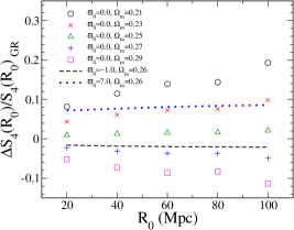
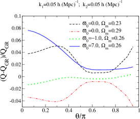
Figure 3 plots $(Q-Q_{\text{GR}})/Q_{\text{GR}}$ for different values of $\varpi_{0}$ and $\Omega_{m}$. $Q_{\text{GR}}$ is the value of the normalized bispectrum (56) in a $\varpi=0$ universe with the WMAP 5-year maximum likelihood cosmology wmapparams . We use a Monte Carlo integrator based on the sobol sequence generator sobseq() presented in reference numericalrecipes to evaluate integral (55). The WMAP 5-year team Dunkley:2008ie reports $\Omega_{m}=0.26\pm 0.03\,(1\sigma)$. Reference Daniel:2009kr finds that CMB data alone gives $\varpi_{0}=1.7{}^{+4.0}_{-2.0}\,(2\sigma)$. We find that the variation in the bispectrum due to a 1$\sigma$ change in $\Omega_{m}$ is comparable to the variation due to a 2$\sigma$ change in $\varpi_{0}$. Thus we conclude that the three-point function will be of little help in constraining the value of $\varpi_{0}$. Even if future experiments improve our constraint on $\Omega_{m}$, the fact that measurements of the galaxy three-point correlation function are only precise to $\gtrsim 10\%$ (see Tables A1-A3 of reference Kulkarni:2007qu ) means that we are a long way off from being able to constrain $\varpi_{0}$ from the distribution of galaxies in the Universe.

V Scale dependence

As was discussed in reference Daniel:2008et , our scale-independent model of gravitational slip (4) does not affect the shape of the power spectrum $P_{\delta}$. Any effect on the bispectrum observed in Figure 3 must therefore be due to the renormalization of second order perturbations relative to first order perturbations in the presence of $\varpi\neq 0$. Clearly, this effect is weaker than that of actually changing the shape of $P_{\delta}$, as varying $\Omega_{m}$ does. Figure 2 plots the effect of varying $\varpi_{0}$ on both the unnormalized second order growth functions $\mathcal{D}^{a}$ and $\mathcal{D}^{b}$ (solid lines) and the normalized second order growth functions $\mathcal{D}^{a}/D^{2}$ and $\mathcal{D}^{b}/D^{2}$ (dashed lines). The normalization greatly reduces the effect of $\varpi_{0}$, lending credence to our hypothesis that the principal effect of scale-independent gravitational slip on the bispectrum is through the same renormalization previously found for the first order growth function Daniel:2009kr . Fortunately, the most popular alternative gravity models all predict scale-dependent effects Hu:2007pj . It is therefore incumbent upon us to consider the effect of including scale dependence in parametrization (3). In this section, we find that scale-dependent $\varpi$ does amplify non-GR modifications to the bispectrum, provided one considers the right combination of $\{k_{1},k_{2},k_{3}\}$.

V.1 Scale-dependent equations of motion

Because we want solar system tests to remain consistent with general relativity Bertotti:2003rm , we will work in Fourier space and impose the constraint that $\varpi\rightarrow 0$ as $k\rightarrow\infty$. In this case, it is an easy matter to calculate the effect of scale-dependent $\varpi$ on our first order results, provided that we rewrite parametrizations (3) and (4) as

$$\tilde{\psi} = (1+\varpi)\tilde{\phi}$$ (57)

$$\varpi = \varpi_{0}\widetilde{K}(k)a^{3}$$ (58)

with the restriction that $\lim_{k\rightarrow\infty}\widetilde{K}(k)=0$.

To first order, the equations of motion for $\{\phi,\delta,\vec{v}\}$ remain unchanged under this reparametrization. The only difference in our results is that, under (58) the growth functions $D$ and $f$ are dependent on the modulus of the wave vector $\vec{k}$ as well as on redshift. To higher orders, the presence of the non-linear source term (16) forces us to reformulate our approach towards calculating the bispectrum.

Our ability to write equations of motion (25)–(28) depended on the separability of equation (15) into scale- and redshift-dependent parts. Using the first order solutions for $\{\phi,\delta,\vec{v}\}$ we were able to write the second order source term (16) as

$$S^{(2)}=D(1+\varpi)f\partial_{i}(\varphi\nabla^{2}\varphi)+\dot{D}^{2}\partial_{ij}(\partial_{i}\varphi\partial_{j}\varphi).$$

Under reparametrization (57), we have

$$S^{(2)} = \int\frac{d^{3}k_{1}d^{3}k_{2}}{(2\pi)^{3}}e^{i\vec{x}(\vec{k}_{1}+\vec{k}_{2})}\Big{\{}D(k_{1})(1+\varpi(k_{2}))f(k_{2})\big{(}k_{1}^{2}\vec{k}_{1}\cdot\vec{k}_{2}+k_{1}^{2}k_{2}^{2}\big{)}$$ (59)

$$\phantom{d^{3}kd^{3}ke^{ix(k+k)}\Big{\{}}+\dot{D}(k_{1})\dot{D}(k_{2})\big{[}k_{1}^{2}k_{2}^{2}+(\vec{k}_{1}\cdot\vec{k}_{2})^{2}+k_{1}^{2}\vec{k_{1}}\cdot\vec{k}_{2}+k_{2}^{2}\vec{k_{1}}\cdot\vec{k_{2}}\big{]}\Big{\}}\tilde{\varphi}(k_{1})\tilde{\varphi}(k_{2}).$$

The integration over wave vectors (stemming from the fact that reparametrization (57) is defined in Fourier space) makes it impossible for us to find a separable solution for $\{\phi^{(2)},\delta^{(2)},\vec{v}^{(2)}\}$. This does not, however, mean that we need be stymied in our attempt to calculate the bispectrum under (57).

Upon inspection of equation (54), we see that the bispectrum accounting for redshift space distortions and galaxy bias is made up of terms of the following types

$$\langle\tilde{\delta}^{(2)}\tilde{\delta}^{(1)}\tilde{\delta}^{(1)}\rangle$$ (60)

$$\langle\tilde{\delta}^{(2)}\tilde{\delta}^{(1)}\partial_{z}\tilde{v}^{(1)}_{z}\rangle$$ (61)

$$\langle\tilde{\delta}^{(2)}\partial_{z}\tilde{v}^{(1)}_{z}\partial_{z}\tilde{v}^{(1)}_{z}\rangle$$ (62)

$$\langle\partial_{z}\tilde{v}^{(2)}_{z}\delta^{(1)}\delta^{(1)}\rangle$$ (63)

$$\langle\partial_{z}\tilde{v}^{(2)}_{z}\delta^{(1)}\partial_{z}\tilde{v}^{(1)}_{z}\rangle$$ (64)

$$\langle\partial_{z}\tilde{v}^{(2)}_{z}\partial_{z}\tilde{v}^{(1)}_{z}\partial_{z}\tilde{v}^{(1)}_{z}\rangle$$ (65)

$$\langle\delta^{(1)}\delta^{(1)}\delta^{(1)}\delta^{(1)}\rangle$$ (66)

$$\langle\delta^{(1)}\delta^{(1)}\partial_{z}\tilde{v}^{(1)}_{z}\partial_{z}\tilde{v}^{(1)}_{z}\rangle$$ (67)

$$\langle\partial_{z}\tilde{v}^{(1)}_{z}\partial_{z}\tilde{v}^{(1)}_{z}\partial_{z}\tilde{v}^{(1)}_{z}\partial_{z}\tilde{v}^{(1)}_{z}\rangle.$$ (68)

As noted above, we can calculate the terms built totally out of first order pieces (66,67,68) exactly as we did in Section IV.1, allowing for the new scale dependence of the relevant growth functions. We can calculate the terms with second order parts by modifying the equations of motion (15) and (17) so as to calculate the ensemble averages $\langle\delta^{(2)}\delta^{(1)}\delta^{(1)}\rangle$, etc. directly (rather than calculating the second order part, multiplying by the first order parts, and then taking the ensemble average). We explain this modification below.

Consider equation (17). If we multiply both sides by two extra factors of $\delta^{(1)}$ take the Fourier transform and take the ensemble average, we have

$$\int d\{\text{Fourier}\}\Big{\{}\langle\ddot{\tilde{\delta}}^{(2)}_{1}\tilde{\delta}^{(1)}_{2}\tilde{\delta}^{(1)}_{3}\rangle+\mathcal{H}\langle\dot{\tilde{\delta}}^{(2)}\tilde{\delta}^{(1)}_{2}\tilde{\delta}^{(1)}_{3}\rangle\Big{\}}=\int d\{\text{Fourier}\}\Big{\{}\langle\tilde{S}^{(2)}_{1}\tilde{\delta}^{(1)}_{2}\tilde{\delta}^{(1)}_{3}\rangle-k_{1}^{2}(1+\varpi)\langle\tilde{\phi}^{(2)}\tilde{\delta}^{(1)}_{2}\tilde{\delta}^{(1)}_{3}\rangle\Big{\}}$$ (69)

where the integral over $d\{\text{Fourier}\}$ stands for an integral over

$$\frac{d^{3}xd^{3}k_{1\dots 3}}{(2\pi)^{6}}e^{i\vec{x}(\vec{k}-\sum_{j=1}^{3}\vec{k}_{j})}$$

which reduces to

$$\frac{d^{3}k_{1\dots 3}}{(2\pi)^{3}}\delta^{3}_{D}(\vec{k}-\vec{k_{1}}-\vec{k_{2}}-\vec{k_{3}})$$ (70)

upon integration over $d^{3}x$. Simple differential calculus allows us to write the integrand of equation (69) as a second order differential equation for

$$\langle\tilde{\delta}^{(2)}\tilde{\delta}^{(1)}\tilde{\delta}^{(1)}\rangle$$

which is exactly the form of terms like (60) in equation (54). For example,

$$\langle\dot{\tilde{\delta}}_{1}^{(2)}\tilde{\delta}^{(1)}_{2}\tilde{\delta}^{(1)}_{3}\rangle = \frac{d}{d\tau}\langle\tilde{\delta}^{(2)}_{1}\tilde{\delta}^{(1)}_{2}\tilde{\delta}^{(1)}_{3}\rangle-\langle\tilde{\delta}^{(2)}_{1}\dot{\tilde{\delta}}^{(1)}_{2}\tilde{\delta}^{(1)}_{3}\rangle-\langle\tilde{\delta}^{(2)}_{1}\tilde{\delta}^{(1)}_{2}\dot{\tilde{\delta}}^{(1)}_{3}\rangle$$ (71)

$$= \frac{d}{d\tau}\langle\tilde{\delta}^{(2)}_{1}\tilde{\delta}^{(1)}_{2}\tilde{\delta}^{(1)}_{3}\rangle-(\frac{\dot{D}_{2}}{D_{2}}+\frac{\dot{D}_{3}}{D_{3}})\langle\delta^{(2)}_{1}\tilde{\delta}^{(1)}_{2}\tilde{\delta}^{(1)}_{3}\rangle$$

where we have used $\tilde{\delta}^{(1)}_{i}=-k_{i}^{2}D(k_{i})\tilde{\varphi}(k_{i})$. We can use equation (15) to write a similar differential equation, which we can evolve to calculate the $\langle\tilde{\phi}^{(2)}\tilde{\delta}^{(1)}\tilde{\delta}^{(1)}\rangle$ term on the right hand side of equation (69). As for the source term in (69), we can use equation (59) to write

$$\langle\tilde{S}^{(2)}\tilde{\delta}^{(1)}\tilde{\delta}^{(1)}\rangle = \int\frac{d^{3}xd^{3}k_{1\dots 4}}{(2\pi)^{15/2}}e^{i\vec{x}(\vec{k}-\sum_{j=1}^{4}\vec{k}_{j}}\Big{\{}\dots\Big{\}}$$ (72)

$$\qquad\times\langle\tilde{\varphi}_{1}\tilde{\varphi}_{2}\tilde{\delta}^{(1)}_{3}\tilde{\delta}^{(1)}_{4}\rangle$$

$$= \int\frac{d^{3}xd^{3}k_{1\dots 4}}{(2\pi)^{15/2}}\delta^{3}_{D}(\vec{k}-\sum_{j=1}^{4}\vec{k}_{j})\Big{\{}\dots\Big{\}}\times\frac{1}{D_{1}D_{2}k_{1}^{2}k_{2}^{2}}P_{1}P_{2}\times\Big{(}\delta^{3}_{D(1+3)}\delta^{3}_{D(2+4)}+\delta^{3}_{D(1+4)}\delta^{3}_{D(2+3)}\Big{)}$$

$$= 2\int\frac{d^{3}k_{1}d^{3}k_{2}}{(2\pi)^{9/2}}\Big{\{}\dots\Big{\}}\times\frac{P_{1}P_{2}}{D_{1}D_{2}k_{1}^{2}k_{2}^{2}}\delta^{3}_{D}(\vec{k})$$

where $\{\dots\}$ represents the combination of $k$ vectors and growth functions in the integrand of equation (59) symmetrized in terms of $\vec{k}_{1}$ and $\vec{k}_{2}$. The $\delta^{3}_{D}(\vec{k})$ in equation (72) means that the right hand side of equation (69) will be zero unless $\vec{k}=0$, which, from the form (70) of the integral measure in equation (69), implies that the left hand side will be zero unless $\vec{k}_{1}+\vec{k}_{2}+\vec{k}_{3}=0$. This is simply the familiar result that the bispectrum is defined only for triangular configurations of $k$ vectors. Noting that

$$\langle\tilde{\delta}^{(2)}_{1}\tilde{\delta}^{(1)}_{2}\partial_{z}\tilde{v}^{(1)}_{3z}\rangle=-\frac{\dot{D}_{3}}{D_{3}}\frac{k_{3z}^{2}}{k_{3}^{2}}\langle\tilde{\delta}^{(2)}_{1}\tilde{\delta}^{(1)}_{2}\tilde{\delta}^{(1)}_{3}\rangle$$ (73)

we are now able to solve for the terms (61) and (62) in equation (54).

To calculate the terms in (54) which involve $\partial_{z}\tilde{v}^{(2)}_{z}$, we use equation (9) to find

$$\tilde{\vec{v}}^{(2)}=-(\vec{\nabla})^{-1}\dot{\tilde{\delta}}^{(2)}-\int\frac{d^{3}k_{1}d^{3}k_{2}}{(2\pi)^{3/2}}\delta^{3}_{D}(\vec{k}-\vec{k}_{1}-\vec{k}_{2})\tilde{\delta}^{(1)}_{1}\tilde{\vec{v}}^{(1)}_{2}.$$ (74)

We can treat the first term on the right hand side of (74) the same way that we treated $\langle\tilde{\delta}^{(2)}\tilde{\delta}^{(1)}\tilde{\delta}^{(1)}\rangle$ terms in equation (69). Note that

$$\langle(\vec{\nabla}^{-1})\dot{\tilde{\delta}}^{(2)}_{1}\tilde{\delta}^{(1)}_{1}\tilde{\delta}^{(1)}_{3}\rangle = \Big{[}\frac{d}{d\tau}-\left(\frac{\dot{D}_{2}}{D_{2}}+\frac{\dot{D}_{3}}{D_{3}}\right)\Big{]}\times\langle(\vec{\nabla}^{-1})\tilde{\delta}^{(2)}_{1}\tilde{\delta}^{(1)}_{2}\tilde{\delta}^{(1)}_{3}\rangle.$$ (75)

The term $\langle(\vec{\nabla}^{-1})\tilde{\delta}^{(2)}_{1}\tilde{\delta}^{(1)}_{2}\tilde{\delta}^{(1)}_{3}\rangle$ can be found by using the same evolution equations we used to find $\langle\tilde{\delta}^{(2)}\tilde{\delta}^{(1)}\tilde{\delta}^{(1)}\rangle$ except eliminating the leading factor of $2$ from the source term (72) and rewriting the $\{\dots\}$ as

$$\Big{\{}\dots\Big{\}} = D(k_{2})f(k_{3})(1+\varpi(k_{3}))k_{2}^{2}k_{3}+\dot{D}(k_{2})\dot{D}(k_{3})(k_{2}^{2}k_{3}+\vec{k}_{2}\cdot\vec{k}_{3}k_{3}).$$ (76)

The factor of $2$ is eliminated because $\langle(\vec{\nabla}^{-1})\tilde{\delta}^{(2)}_{1}\tilde{\delta}^{(1)}_{2}\tilde{\delta}^{(1)}_{3}\rangle$ is not symmetric in its wave vector arguments. We will need to account for this by summing over all possible arrangements of $\{\vec{k}_{1},\vec{k}_{2},\vec{k}_{3}\}$ when we calculate the bispectrum. The new scale dependence (76) is to account for the inverse $\nabla$ operator. Once the equations of motion have been integrated, we must also multiply by a factor of $-k_{1z}k_{3z}/k_{3}$ to account for the fact that we are interested in the $\partial_{z}$ derivative of the $z$-component of $\vec{v}^{(2)}$.

The second term on the right hand side of (74) is found (relatively) simply from the first order solutions for $\vec{v}$ and $\delta$. Again, we ultimately want to find a term that looks like $\langle\partial_{z}\tilde{v}^{(2)}_{1z}\tilde{\delta}^{(1)}_{2}\tilde{\delta}^{(1)}_{3}\rangle$. Our first order solutions give

$$\text{FT}\partial_{z}\left(\delta^{(1)}_{4}v^{(1)}_{5z}\right) = i\int\frac{d^{3}k_{4}d^{3}k_{5}}{(2\pi)^{3/2}}\delta^{3}_{D}(\vec{k}-\vec{k}_{4}-\vec{k}_{5})(k_{4z}+k_{5z})\tilde{\delta}^{(1)}_{4}\tilde{v}^{(1)}_{5z}$$

$$= -\int\frac{d^{3}k_{4}d^{3}k_{5}}{(2\pi)^{3/2}}\delta^{3}_{D}(\vec{k}-\vec{k}_{4}-\vec{k}_{5})(k_{4z}+k_{5z})\frac{\dot{D}_{5}}{D_{5}}\frac{k_{5z}}{k_{5}^{2}}\tilde{\delta}^{(1)}_{4}\tilde{\delta}^{(1)}_{5}$$

where FT denotes a Fourier transform. From here we see that $\text{FT}\langle\partial_{z}\left(\delta^{(1)}v^{(1)}\right)\tilde{\delta}^{(1)}\tilde{\delta}^{(1)}\rangle$ will contribute terms like

$$-P_{2}P_{3}\frac{k_{3z}k_{1z}}{k_{3}^{2}}\frac{\dot{D}_{3}}{D_{3}}$$

to the bispectrum. This contribution can be added to the contribution (75) to find that, the $\langle\partial_{z}\tilde{v}^{(2)}_{z}\tilde{\delta}^{(1)}\tilde{\delta}^{(1)}\rangle$ term in the redshift distortion-corrected bispectrum will be

$$\langle\partial_{z}\tilde{v}^{(2)}_{z}\tilde{\delta}^{(1)}\tilde{\delta}^{(1)}\rangle = \sum\frac{k_{3z}k_{1z}}{k_{3}}\Big{\{}-\left[\frac{d}{d\tau}-\left(\frac{\dot{D}_{2}}{D_{2}}+\frac{\dot{D}_{3}}{D_{3}}\right)\right]\langle(\vec{\nabla}^{-1})\tilde{\delta}^{(2)}_{1}\tilde{\delta}^{(1)}_{2}\tilde{\delta}^{(1)}_{3}\rangle+\frac{\dot{D}_{3}}{k_{3}D_{3}}P_{2}P_{3}\Big{\}}$$ (77)

where the sum is over the 6 permutations of $\{\vec{k}_{1},\vec{k}_{2},\vec{k}_{3}\}$. This is the term (63) in equation (54). Using equation (73), we can also evaluate terms (64) and (65). Thus, we are able to calculate the redshift distortion-corrected bispectrum in the case of scale-dependent gravitational slip.

Because our source term (59) depends on the power spectrum at specific length scales we cannot, as in Section II, evolve our equations of motion (69) from arbitrarily early times without regards to the shape of $\{\tilde{\phi}^{(1)},\tilde{\delta}^{(1)}\}$ and then add the scale-dependence later. We must, instead, begin with realistic initial conditions for the perturbation modes. Since the form of (58) is such that $\lim_{a\rightarrow 0}\varpi=0$, we take these initial conditions from the Boltzmann code CMBfast Seljak:1996is with the appropriate background parameters and modified it to output $\{\tilde{\phi}^{(1)},\dot{\tilde{\phi}}^{(1)},\tilde{\delta}^{(1)},\dot{\tilde{\delta}}^{(1)}\}$ at $a=0.1$ (chosen as an epoch early enough that $\varpi\sim 0$ and late enough that quasi-linear structure growth can be expected to set in). We still assume that $\tilde{\phi}^{(2)}=\dot{\tilde{\phi}}^{(2)}=\tilde{\delta}^{(2)}=\dot{\tilde{\delta}}^{(2)}=0$ at this initial epoch. With these initial conditions, we can calculate the redshift distortion-corrected bispectrum (54) in the case of scale-dependent $\varpi$. All that remains is to explore the effect of parametrization (57) on obsevable statisitics.

V.2 Effects on observables

To compare the effects of scale-dependent gravitational slip to a $\varpi=0$ universe, we perform the same average over orientation as in equation (55) and use the same $Q$ statistic as defined in equation (56). The denominator of $Q$ in the case of scale-dependent gravitational slip is written

$$b_{1}^{4}(P_{1}P_{2}a_{1}a_{2}+P_{1}P_{3}a_{1}a_{3}+P_{2}P_{3}a_{2}a_{3})$$

with

$$a_{i} \equiv 1+\frac{2}{3}f_{1,i}+\frac{1}{5}f_{1,i}^{2}$$

$$f_{1,i} \equiv \frac{a}{D(k_{i})}\frac{dD(k_{i})}{da}.$$

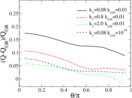
Figure 4 plots the effect of scale-dependent $\varpi$ on the $Q$ statistic. For the purposes of this plot, we choose $\varpi$ to have a scale dependence given by (recall equation 58)

$$\widetilde{K}(k)=\frac{1+\frac{k}{k_{\text{crit}}}}{1+0.01\left(\frac{k}{k_{\text{crit}}}\right)^{2}}.$$ (78)

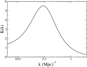
In Figure 4 we choose $k_{\text{crit}}=0.01(\text{Mpc})^{-1}$ and $\varpi_{0}=5$. This is an illustrative model only and is not meant to represent any specific theory of gravity. Including the scale dependence (78) amplifies the effect of gravitational slip on $Q$, but only for configurations $\{\vec{k}_{1},\vec{k}_{2},\vec{k}_{3}\}$ in which the length scales correspond to the peak of $\widetilde{K}(k)$. It therefore seems reasonable to conclude that, while the bispectrum may be able to tell us something about scale-dependent gravitational slip, it will only do so if we choose to examine a particularly sensitive range of $k$.

Figure 4: The same as Figure 3 except for scale-dependent $\varpi$ of the form (58) with $\varpi_{0}=5$ and $\widetilde{K}(k)$ given by equation (78). All length scales are in units of Mpc. All triangles considered are isosceles (i.e., $k_{2}=k_{1}$). As in Figure 3, $\theta$ is the angle between $\vec{k}_{1}$ and $\vec{k}_{2}$. Figure 4 plots $\widetilde{K}(k)$. Figure 4 plots the change in the bispectrum relative to the WMAP5 maximum likelihood GR cosmology wmapparams for different triangles. The case of $k_{\text{crit}}=10^{14}$ is shown to illustrate what the curve would look like for scale-independent $\varpi$ (4). The effect of $\varpi$ is much more pronounced for triangles whose sides correspond to length scales at which $\widetilde{K}(k)$ peaks.

VI Conclusion

Contrary to expectations, we have found that quasi-linear order structure growth is ineffective at constraining scale-independent gravitational slip (4). However, with judicious triangle choice, we may be able to say something about a scale-dependent gravitational slip (58) by measuring the bispectrum. To date, there has been no attempt to constrain scale-dependent gravitational slip with even linear-order cosmological data. Conventional wisdom has been that the data is still too imprecise to say anything meaningful about so detailed an effect as scale-dependence. The next generation of cosmological experiments will hopefully remedy this oversight Daniel:2009kr . Given the prevalence of scale-dependent effects in alternative gravity theories Hu:2007pj , it may behoove us to find a useful, model-independent parametrization of the scale dependence $\widetilde{K}(k)$ (58) and subject these future datasets to the same analysis given in reference Daniel:2009kr . Depending on what such investigations say, the results of Section V may be able to extend our knowledge by bringing to bear measurements of the three-point correlation function on the question of gravitational slip.

Appendix A Comparison to Lagrangian perturbation theory

Equation (54) was derived using Eulerian perturbation theory (i.e., we evolved the perturbed fields $\{\phi,\delta,\vec{v}\}$ directly). Hivon et al. Hivon:1994qb perform the same calculation using the Lagrangian perturbation theory formalism laid out in references Bouchet:1992xz ; Bouchet:1994xp ; Buchert:1992ya ; Buchert:1993xz . Rather than evolving the perturbed density and velocity fields, Lagrangian perturbation theory evolves the displacement field $\vec{\Psi}(\tau,\vec{q})$ defined as the displacement of a fluid element whose initial position in space was $\vec{q}$. Put another way, at some time $\tau$, the position of a fluid element originating at spatial position $\vec{q}$ and initial time $\tau_{i}$ is

$$\vec{x}=\vec{q}+\vec{\Psi}(\tau-\tau_{i},\vec{q}).$$ (79)

From this, we find that the perturbed velocity field of Section II is just

$$\vec{v} = \frac{d\vec{x}}{d\tau}=\dot{\vec{\Psi}}(\tau,\vec{q})+(\vec{v}\cdot\vec{\nabla})\vec{\Psi}(\tau,\vec{q})$$ (80)

$$= \dot{\vec{\Psi}}^{(1)}+(\dot{\vec{\Psi}}^{(1)}\cdot\vec{\nabla})\vec{\Psi}^{(1)}+\dot{\vec{\Psi}}^{(2)}+\mathcal{O}(3)$$

where we have set $\tau_{i}\equiv 0$. Note that in our notation (as in Section II), an overdot denotes partial differentiation with respect to conformal time $\tau$. In Hivon et al’s notation, an overdot denotes the Lagrangian derivative $(\partial_{\tau}+\vec{v}\cdot\vec{\nabla})$. The same conservation of mass considerations that prompted us to write equation (46), now imply

$$\bar{\rho}(1+\delta)d^{3}x=\bar{\rho}d^{3}q.$$

There is no $\delta$ on the right hand side because we assume that the fluid starts from a homogeneous state. Algebra and equation (79) give

$$\delta = |\frac{d^{3}q}{d^{3}x}|-1=\bigg{(}1+\vec{\nabla}\cdot\vec{\Psi}^{(1)}+\frac{1}{2}\Big{[}(\vec{\nabla}\cdot\vec{\Psi}^{(1)})^{2}-\partial_{i}\Psi^{(1)}_{j}\partial_{j}\Psi^{(1)}_{i}\Big{]}+\vec{\nabla}\cdot\vec{\Psi}^{(2)}+\mathcal{O}(3)\bigg{)}^{-1}$$ (81)

$$= -\vec{\nabla}\cdot\vec{\Psi}^{(1)}+(\vec{\nabla}\cdot\vec{\Psi}^{(1)})^{2}-\vec{\nabla}\cdot\vec{\Psi}^{(2)}-\frac{1}{2}\Big{[}(\vec{\nabla}\cdot\vec{\Psi}^{(1)})^{2}-\partial_{i}\Psi^{(1)}_{j}\partial_{j}\Psi^{(1)}_{i}\Big{]}+\mathcal{O}(3)$$

where we have expanded $\Psi$ in the same way that we expanded $\phi$, $\delta$ and $\vec{v}$ in Section II. With equations (80) and (81), we can find the same physical quantities in Lagrangian perturbation theory (LPT) as we calculated directly in Eulerian perturbation theory (EPT) in Section II. The advantage is that, in LPT, the transition to redshift space is merely a coordinate transformation. In this section, we show that our EPT results are consistent with LPT results to second order. In reference Bernardeau:2001qr , Bernardeau claims that this is not the case, that LPT and EPT do not agree and that LPT is more consistent with the results of N-body simulations (see the discussion following his Figure 48). This is merely a confusion of terminology. What Bernardeau meant to claim is that second order LPT and EPT results differ substantially from third order LPT results (the difference between “tree-level” and “one-loop level” perturbation theory in reference Scoccimarro:1996jy ) and that N-body simulations are more consistent with the third order results. In Section IV, we found that the effect of $\varpi_{0}$ on the second order results is not strong enough to justify extending our calculations out to higher order.

Before we begin, there is a subtlety which bears discussion. All of the $\vec{\Psi}$ functions and their spatial derivatives in equations (80) and (81) are expressed in terms of $\vec{q}$ coordinates, that is, in terms of the spatial positions of fluid elements at initial time $\tau=0$. When we go to derive field equations for $\phi$ and $\vec{\Psi}$, we will be expressing $\phi$ and its spatial derivatives in terms of $\vec{x}$ coordinates (spatial positions now). Assume that $\Psi_{j}\ll q_{j}$. Because we will only be interested in quantities up to second order, the transformation between $\vec{q}$ and $\vec{x}$ coordinates is a straightforward Taylor expansion. If we use $\vec{\bar{\Psi}}(\vec{x})$ to represent the displacement field as a function of the present position $\vec{x}$ (see reference Hivon:1994qb ), then

$$\vec{\Psi}(\vec{q}) = \vec{\bar{\Psi}}(\vec{x})+\partial_{x_{i}}\vec{\bar{\Psi}}(\vec{x})(\vec{q}-\vec{x})_{i}+\mathcal{O}(\vec{\bar{\Psi}}^{3})$$ (82)

$$= \vec{\bar{\Psi}}(\vec{x})-\bar{\Psi}_{i}\partial_{x_{i}}\vec{\bar{\Psi}}(\vec{x})+\mathcal{O}(\vec{\bar{\Psi}}^{3})$$

$$\partial_{q}\vec{\Psi}(\vec{q}) = \frac{\partial x}{\partial q}\partial_{x}\Big{(}\vec{\bar{\Psi}}(\vec{x})-\bar{\Psi}_{i}\partial_{x_{i}}\vec{\bar{\Psi}}(\vec{x})+\mathcal{O}(\vec{\bar{\Psi}}^{3})\Big{)}$$ (83)

$$= \Big{(}1+\partial_{q}\vec{\Psi}\Big{)}\cdot\Big{(}\partial_{x}\vec{\bar{\Psi}}-\partial_{x}\bar{\Psi}_{i}\partial_{x_{i}}\vec{\bar{\Psi}}-\bar{\Psi}_{i}\partial_{x}\partial_{x_{i}}\vec{\bar{\Psi}}+\mathcal{O}(\vec{\bar{\Psi}}^{3})\Big{)}$$

$$= \nabla_{x}\vec{\bar{\Psi}}-\bar{\Psi}_{i}\partial_{x}\partial_{x_{i}}\vec{\bar{\Psi}}+\mathcal{O}(\vec{\bar{\Psi}}^{3})$$

where we have used the zeroth order equation $\vec{q}=\vec{x}$. Now

$$\delta = -\vec{\nabla}\cdot\vec{\bar{\Psi}}^{(1)}+(\vec{\bar{\Psi}}\cdot\vec{\nabla})\vec{\nabla}\cdot\vec{\bar{\Psi}}+(\vec{\nabla}\cdot\vec{\bar{\Psi}}^{(1)})^{2}-\frac{1}{2}((\vec{\nabla}\cdot\bar{\Psi}^{(1)})^{2}-\partial_{i}\bar{\Psi}^{(1)}_{j}\partial_{j}\bar{\Psi}^{(1)}_{i})-\vec{\nabla}\cdot\vec{\bar{\Psi}}^{(2)}+\mathcal{O}(3)$$ (84)

$$\vec{v} = \dot{\vec{\bar{\Psi}}}^{(1)}-\dot{\bar{\Psi}}^{(1)}_{i}\partial_{i}\vec{\bar{\Psi}}^{(1)}-\bar{\Psi}_{i}^{(1)}\partial_{i}\dot{\vec{\bar{\Psi}}}^{(1)}+\dot{\vec{\bar{\Psi}}}_{i}^{(1)}\partial_{i}\vec{\bar{\Psi}}^{(1)}+\dot{\vec{\bar{\Psi}}}^{(2)}+\mathcal{O}(3)$$ (85)

$$= \dot{\vec{\bar{\Psi}}}^{(1)}-\bar{\Psi}_{i}^{(1)}\partial_{i}\dot{\vec{\bar{\Psi}}}^{(1)}+\dot{\vec{\bar{\Psi}}}^{(2)}+\mathcal{O}(3).$$

From here on, we will deal only in $\vec{\bar{\Psi}}(\vec{x})$ and derivatives with respect to $\vec{x}$. Let us now consider the LPT equations of motion.

LPT proceeds from the geodesic equation

$$u^{\alpha}\nabla_{\alpha}u^{i}=0$$

($i$ is a spatial index) and the Poisson equation. We once again replace the Poisson equation with the space-time Einstein equation in the form (13)

$$\nabla^{2}\left(\dot{\phi}+\mathcal{H}(1+\varpi)\phi\right)=\frac{3}{2}\mathcal{H}^{2}\Omega_{m}\dot{\delta}$$

with $\delta$ taken from equation (84) so that, to first order,

$$\frac{3}{2}\mathcal{H}^{2}\Omega_{m}\Big{(}\vec{\nabla}\cdot\dot{\vec{\bar{\Psi}}}^{(1)}\Big{)}=-\nabla^{2}\left(\dot{\phi}+\mathcal{H}(1+\varpi)\phi\right).$$ (86)

Using metric (7) and four-velocity (8), the geodesic equation taken out to zeroth order in $1/c^{2}$ merely returns equation (10)

$$\dot{\vec{v}}+\mathcal{H}\vec{v}+(\vec{v}\cdot\vec{\nabla})\vec{v}+\vec{\nabla}\phi(1+\varpi)=0.$$

To first order in $\{\phi,\delta,\vec{v}\}$, this equation gives

$$-\nabla^{2}\psi = \vec{\nabla}\cdot\dot{\vec{v}}+\mathcal{H}\vec{\nabla}\cdot\vec{v}$$ (87)

$$= \vec{\nabla}\cdot\ddot{\vec{\bar{\Psi}}}^{(1)}+\mathcal{H}\vec{\nabla}\cdot\dot{\vec{\bar{\Psi}}}^{(1)}$$

where we have used equation (85). The time derivative of equation (86) gives

$$\frac{3}{2}\mathcal{H}^{2}\Omega_{m}\Big{(}\vec{\nabla}\cdot\ddot{\vec{\bar{\Psi}}}^{(1)}-\mathcal{H}\vec{\nabla}\cdot\dot{\vec{\bar{\Psi}}}^{(1)}\Big{)} = -\nabla^{2}\Big{(}\ddot{\phi}+\dot{\mathcal{H}}(1+\varpi)\phi+\mathcal{H}(1+\varpi)\dot{\phi}+\mathcal{H}\dot{\varpi}\phi\Big{)}$$

$$\frac{3}{2}\mathcal{H}^{2}\Omega_{m}\Big{(}\vec{\nabla}\cdot\ddot{\vec{\bar{\Psi}}}^{(1)}+\mathcal{H}\vec{\nabla}\cdot\dot{\vec{\bar{\Psi}}}^{(1)}\Big{)}-3\mathcal{H}^{3}\Omega_{m}\vec{\nabla}\cdot\dot{\vec{\bar{\Psi}}}^{(1)} =$$

$$\frac{3}{2}\mathcal{H}^{2}\Omega_{m}\left(-\nabla^{2}\phi(1+\varpi)\right)+2\mathcal{H}\nabla^{2}\left(\dot{\phi}+\mathcal{H}(1+\varpi)\phi\right) =$$ (88)

where, in the last line, we substitute from equations (86) and (87). Equation (88) can be rearranged to give the first order EPT equation (15). Clearly, the first order result for $\phi$ is identical in either LPT or EPT formalism. The same is true of $\delta$ and $\vec{v}$, given that equations (84) and (85) give $\dot{\delta}=-\vec{\nabla}\cdot\vec{v}$, which is the first order part of the EPT equation of motion (9). To second order, we illustrate the consistency between LPT and EPT by observing that the second order parts of equations (84) and (85) are such that

$$\dot{\delta}^{(2)} = \partial_{i}\bar{\Psi}_{i}^{(1)}\partial_{j}\dot{\bar{\Psi}}_{j}^{(1)}+\dot{\bar{\Psi}}_{i}\partial_{ij}\bar{\Psi}_{j}+\bar{\Psi}_{i}^{(1)}\partial_{ij}\dot{\bar{\Psi}}_{j}^{(1)}+\partial_{i}\dot{\bar{\Psi}}^{(1)}_{j}\partial_{j}\bar{\Psi}_{i}^{(1)}-\partial_{i}\dot{\bar{\Psi}}_{i}^{(2)}$$ (89)

$$= -\partial_{i}v^{(2)}_{i}+\partial_{i}\bar{\Psi}_{i}^{(1)}\partial_{j}\dot{\bar{\Psi}}^{(1)}_{j}+\dot{\bar{\Psi}}^{(1)}_{i}\partial_{ij}\bar{\Psi}^{(1)}_{j}$$

$$= -\partial_{i}v^{(2)}_{i}-\delta^{(1)}\partial_{i}v^{(1)}_{i}-v^{(1)}_{i}\partial_{i}\delta^{(1)}$$

which is the second order part of equation (9). Note that we have used the assumption that the fluid flow is irrotational so that $\partial_{i}\bar{\Psi}_{j}=\partial_{j}\bar{\Psi}_{i}$. Using result (89) as motivation, we will now write the growth functions from reference Hivon:1994qb in terms of our own and show that our second order solutions are, indeed, equivalent to those of LPT.

Results in reference Hivon:1994qb are presented in terms of the growth factors $g_{1}$ and $g_{2}$ and their dimensionless derivatives $f_{i}=(a/g_{i})(dg_{i}/da)$. These growth factors are defined such that

$$\bar{\Psi}=g_{1}\tilde{\bar{\Psi}}^{(1)}+g_{2}\tilde{\bar{\Psi}}^{(2)}$$

where $\tilde{\bar{\Psi}}$ denotes the spatial part of $\bar{\Psi}$. From the first order part of equation (81), it is easy to see that $g_{1}$ is just our growth factor $D$ from equation (19). To find $g_{2}$ as a function of our second order growth functions $\mathcal{D}^{a}$ and $\mathcal{D}^{b}$, we compare our equation (41) to equation (A19) of reference Hivon:1994qb , which finds that $\delta$ goes as

$$\delta^{(2)} = g_{1}^{2}\int\frac{d^{3}k_{1}d^{3}k_{2}}{(2\pi)^{3}}\tilde{\phi}^{(1)}_{1}\tilde{\phi}^{(1)}_{2}k_{1}^{2}k_{2}^{2}W(|\vec{k}_{1}+\vec{k}_{2}|)e^{i\vec{x}\cdot(\vec{k}_{1}+\vec{k}_{2})}\Big{(}1+\cos\theta_{12}\frac{k_{1}}{k_{2}}-(1+\frac{g_{2}}{g_{1}^{2}})\frac{(1-\cos^{2}\theta_{12})}{2}\Big{)}.$$ (90)

The comparison with our equation (41) proceeds more directly if we write

$$\mathcal{D}^{a} = -2D_{1}^{2}+\frac{3}{2}D_{2}$$

$$\mathcal{D}^{b} = \frac{3}{2}D_{1}^{2}-\frac{3}{4}D_{2}$$

where $D_{1}$ is just the first order growth function $D$ from equation (19), and $D_{2}$ is defined in equation (39a) of reference Bernardeau:1993qu (this equivalence can be seen by comparing that work’s equation 48 with our equation 41). Now, we can rewrite our equation as

$$\delta^{(2)} = \int\frac{d^{3}k_{1}d^{3}k_{2}}{(2\pi)^{3}}\tilde{\phi}^{(1)}_{1}\tilde{\phi}^{(1)}_{2}k_{1}^{2}k_{2}^{2}e^{i\vec{x}\cdot(\vec{k}_{1}+\vec{k}_{2})}$$ (91)

$$\qquad\times\Big{(}(-2D_{1}^{2}+\frac{3}{2}D_{2})(1+\frac{k_{1}}{k_{2}}\cos\theta_{12})+(\frac{3}{2}D_{1}^{2}-\frac{3}{4}D_{2})(1+\cos^{2}\theta_{12}+2\frac{k_{1}}{k_{2}}\cos\theta_{12})\Big{)}.$$

Comparing equations (90) and (91), we find that $D_{1}=g_{1}$ (as promised) and

$$g_{2}=2D_{1}^{2}-\frac{3}{2}D_{2}$$

or

$$g_{2}=-3\mathcal{D}^{a}-4\mathcal{D}^{b}+2D_{1}^{2}$$ (92)

or

$$\mathcal{D}^{a} = -g_{2}$$ (93)

$$\mathcal{D}^{b} = \frac{1}{2}(D^{2}+g_{2}).$$ (94)

Using these results and equation (22), we find for EPT

$$\vec{\nabla}\cdot\vec{v}^{(2)}_{\text{EPT}} = (\dot{g}_{2}+D\dot{D})(\nabla^{2}\varphi\nabla^{2}\varphi+\partial_{i}\varphi\partial_{i}\nabla^{2}\varphi)-(\dot{g}_{2}/2+D\dot{D})(\nabla^{2}\varphi\nabla^{2}\varphi+\partial_{ij}\varphi\partial_{ij}\varphi+2\partial_{j}\varphi\partial_{j}\nabla^{2}\varphi)$$

$$= \frac{\dot{g}_{2}}{2}(\nabla^{2}\varphi\nabla^{2}\varphi-\partial_{ij}\varphi\partial_{ij}\varphi)-D\dot{D}(\partial_{ij}\varphi\partial_{ij}\varphi+\partial_{i}\varphi\partial_{i}\nabla^{2}\varphi).$$

For LPT, we note that $\delta^{(1)}=-\partial_{i}\bar{\Psi}^{(1)}_{i}$ means that $\bar{\Psi}^{(1)}_{i}=-D\partial_{i}\varphi$. This, combined with the result from reference Hivon:1994qb that

$$\partial_{i}\bar{\Psi}^{(2)}_{i}=\frac{g_{2}}{g_{1}^{2}}\frac{1}{2}\Big{[}(\partial_{i}\bar{\Psi}_{i}^{(1)})^{2}-\partial_{i}\bar{\Psi}_{j}^{(1)}\partial_{j}\bar{\Psi}_{i}^{(1)}\Big{]}$$ (95)

gives

$$\vec{\nabla}\cdot\vec{v}^{(2)}_{\text{LPT}} = \frac{1}{2}(\frac{\dot{g}_{2}}{g_{1}^{2}}-2\dot{g}_{1}\frac{g_{2}}{g_{1}^{3}})\Big{[}(\partial_{i}\bar{\Psi}^{(1)})^{2}-\partial_{i}\bar{\Psi}^{(1)}_{j}\partial_{j}\bar{\Psi}^{(1)}_{i}\Big{]}+\dot{g}_{1}\frac{g_{2}}{g_{1}^{3}}\Big{[}(\partial_{i}\bar{\Psi}^{(1)})^{2}-\partial_{i}\bar{\Psi}^{(1)}_{j}\partial_{j}\bar{\Psi}^{(1)}_{i}\Big{]}-\partial_{j}(\bar{\Psi}^{(1)}_{i}\partial_{i}\dot{\bar{\Psi}}^{(1)}_{j})$$

$$= \frac{\dot{g}_{2}}{2}(\nabla^{2}\varphi\nabla^{2}\varphi-\partial_{ij}\varphi\partial_{ij}\varphi)-D\dot{D}(\partial_{ij}\varphi\partial_{ij}\varphi+\partial_{j}\varphi\partial_{j}\nabla^{2}\varphi).$$

From this we see that equation (92), which guarantees $\delta^{(2)}_{\text{LPT}}=\delta^{(2)}_{\text{EPT}}$ also provides $\vec{v}^{(2)}_{\text{LPT}}=\vec{v}^{(2)}_{\text{EPT}}$. Figure 5 compares the results of Section IV with the results of LPT in the case of $\varpi=0$. LPT results are evaluated from Hivon et al’s equations (33)-(35) using our equation (92). We find that our EPT results agree with Hivon et al’s LPT results at the sub-percent level.

Figure 5: We plot the relative disagreement in $\mathcal{B}_{\text{avg}}$ between Eulerian and Lagrangian (reference Scoccimarro:2000sp ; Hivon:1994qb ) perturbation theories. The horizontal axes are the angle of separation between the vectors $\vec{k}_{1}$ and $\vec{k}_{2}$ in units of $\pi$. The vertical axes are $(\mathcal{B}_{\text{avg, EPT}}-\mathcal{B}_{\text{avg, LPT}})/\mathcal{B}_{\text{avg,LPT}}$. We compare (55) with $b_{1}=1$ and $b_{2}=0$ to the results presented in equations (33)-(35) of reference Hivon:1994qb . We use equation (92) to express $g_{2}$ and $f_{2}=(a/g_{2})(dg_{2}/da)$ in terms of our growth functions. For all curves, $\varpi_{0}=0$ and the background cosmology is the WMAP 5-year maximum likelihood universe Dunkley:2008ie ; wmapparams .

Figure 6: We plot the departure of $\mathcal{D}^{a}$ from the predictions of equation (96) as a function of $\varpi_{0}$ for different $\Omega_{m}$ cosmologies. While equation (96) holds exactly when $\varpi_{0}=0$, the relationship breaks down as $|\varpi_{0}|$ grows.

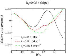
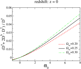
All of the discussion in this Appendix has assumed $\varpi=0$. As shown above, our results are perfectly consistent with LPT in this limit. One can move between the two formalisms using the algebraic relationships (93) and (94). This is not the case once $\varpi_{0}\neq 0$. Equations (93) and (94) imply a relationship between $\mathcal{D}^{a}$, $\mathcal{D}^{b}$, and $D$. Specifically, they imply

$$\mathcal{D}^{a}=-2\mathcal{D}^{b}+D^{2}.$$ (96)

Figure 6 plots the departure from this relationship as a function of $\varpi_{0}$ for cosmologies with different values of $\Omega_{m}$. All of the curves are evaluated at redshift $z=0$. While we see that equation (96) is identically true for $\varpi_{0}=0$, it becomes less and less true as $|\varpi_{0}|$ grows. Recall that equations (93) and (94) were derived by assuming that $\delta^{(2)}_{\text{LPT}}=\delta^{(2)}_{\text{EPT}}$ and comparing the growth functions of the different spatially dependent terms. If we assume that LPT and EPT remain in agreement for $\varpi_{0}\neq 0$, it seems likely that the spatial dependence of $\delta^{(2)}$ must change for $\varpi_{0}\neq 0$. Specifically the spatial relationship (95) may break down, spoiling the relationship between our EPT growth factors and the LPT growth factor $g_{2}$. Given our success at reproducing the $\varpi_{0}=0$ solutions of LPT, the main body of this paper analyzed the $\varpi_{0}\neq 0$ bispectrum using our EPT solutions. It may be worth solving the exact $\varpi_{0}\neq 0$ LPT equations of motion in some future work.

Appendix B The skewness

The third order moment (the skewness) is a measure of the asymmetry of the $\delta$ distribution function once non-linear growth has set in. Mathematically, it is defined as

$$S_{3}=\frac{\langle\delta^{3}(\vec{x})\rangle}{\langle\delta^{2}(\vec{x})\rangle^{2}}\\$$ (97)

Kamionkowski and Buchalter derive an exact expression for the skewness of the matter distribution in a general relativistic universe under different assumptions of flatness and acceleration or deceleration Kamionkowski:1998fv . In this section, we follow their lead and derive a similar expression in the case of $\varpi_{0}\neq 0$.

As with the bispectrum, the numerator of the skewness (97) reduces to $3\langle\delta^{(2)}(\delta^{(1)})^{2}\rangle$. Equation (41) gives us

$$\langle\delta^{(2)}(\delta^{(1)})^{2}\rangle = \int\frac{d^{3}k_{1}\dots d^{3}k_{4}}{(2\pi)^{6}}e^{i\vec{x}\cdot(\vec{k}_{1}+\vec{k}_{2}+\vec{k}_{3}+\vec{k}_{4})}\frac{\langle\tilde{\delta}_{1}\tilde{\delta}_{2}\tilde{\delta}_{3}\tilde{\delta}_{4}\rangle}{D^{2}k_{3}^{2}k_{4}^{2}}$$ (98)

$$\qquad\times\Bigg{[}\vec{k}_{3}\cdot\vec{k_{4}}k^{2}_{4}(\mathcal{D}^{a}+2\mathcal{D}^{b})+k_{3}^{2}k_{4}^{2}(\mathcal{D}^{a}+\mathcal{D}^{b})+(\vec{k}_{3}\cdot\vec{k}_{4})^{2}\mathcal{D}^{b}\Bigg{]}.$$

Using the following results

$$\int\frac{d^{2}k_{1}d^{3}k_{2}}{(2\pi)^{6}}\frac{P_{\delta}(k_{1})P_{\delta}(k_{2})}{D^{2}}\Big{(}-2k_{1}^{2}\vec{k}_{1}\cdot\vec{k}_{2}-1\Big{)} = -\int\frac{d^{2}k_{1}d^{3}k_{2}}{(2\pi)^{6}}\frac{P_{\delta}(k_{1})P_{\delta}(k_{2})}{D^{2}}$$ (99)

$$\int\frac{d^{2}k_{1}d^{3}k_{2}}{(2\pi)^{6}}\frac{P_{\delta}(k_{1})P_{\delta}(k_{2})}{D^{2}}\Big{(}1+2\frac{(\vec{k}_{1}\cdot\vec{k}_{2})^{2}}{k_{1}^{2}k_{2}^{2}}\Big{)} = \int\frac{d^{2}k_{1}d^{3}k_{2}}{(2\pi)^{6}}\frac{P_{\delta}(k_{1})P_{\delta}(k_{2})}{D^{2}}\Big{(}1+2\cos^{2}\theta_{12}\Big{)}$$

$$\int_{-1}^{1}d(\cos\theta)\cos^{2}\theta = \frac{2}{3}$$

$$\int\frac{d^{2}k_{1}d^{3}k_{2}}{(2\pi)^{6}}\frac{P_{\delta}(k_{1})P_{\delta}(k_{2})}{D^{2}}\Big{(}1+2\cos^{2}\theta_{12}\Big{)} = \frac{5}{3}\int\frac{d^{2}k_{1}d^{3}k_{2}}{(2\pi)^{6}}\frac{P_{\delta}(k_{1})P_{\delta}(k_{2})}{D^{2}}$$ (100)

we find that the normalized skewness may be written

$$S_{3}=\frac{3\langle\delta^{(2)}(\delta^{(1)})^{2}\rangle}{\langle(\delta^{(1)})^{2}\rangle^{2}}=\frac{3}{D^{2}}\left(2\mathcal{D}^{a}+\frac{8}{3}\mathcal{D}^{b}\right).$$ (101)

Note that the denominator of the left hand side of equation (101) is effectively

$$\int\frac{d^{3}k_{1}d^{3}k_{2}}{(2\pi)^{6}}P_{\delta}(k_{1})P_{\delta}(k_{2})$$

hence the simplicity of the right hand side.

Figure 7: We plot the change in the skewness $S_{3}$ (97) resulting from varying $\Omega_{m}$ and $\varpi_{0}$. When $\Omega_{m}$ is varied, $\varpi_{0}=0$. When $\varpi_{0}$ is varied, $\Omega_{m}=0.256$. $\Delta S_{3}$ is assessed relative to a $\varpi_{0}=0,\Omega_{m}=0.256$ universe. All other parameters are set to be the WMAP 5-year maximum likelihood values Dunkley:2008ie . Over regions of interest, the effect of varying $\varpi_{0}$ is much stronger than the effect of varying $\Omega_{m}$. Unfortunately, this will not hold when the calculation is altered to take into account a realistic observational window function (see Figure 8).

Figures 7 and 7 plot the effect of the parameters $\Omega_{m}$ and $\varpi_{0}$ on the skewness as determined by equation (101). When $\Omega_{m}$ is varied, $\varpi_{0}=0$. When $\varpi_{0}$ is varied, $\Omega_{m}=0.256$. All other parameters are set to be the WMAP 5-year maximum likelihood values Dunkley:2008ie . As in Figure 3, the vertical axis is

$$\frac{\Delta S_{3}}{S_{3,\text{GR}}}=\frac{S_{3}-S_{3|\varpi_{0}=0,\Omega_{m}=0.256}}{S_{3|\varpi_{0}=0,\Omega_{m}=0.256}}.$$ (102)

Varying $\varpi_{0}$ within the WMAP 5-year 2$\sigma$ limit ($\varpi_{0}=1.4^{+4.0}_{-2.0}\,(2\sigma)$ Daniel:2009kr ) results in a few percent variation in $S_{3}$, while, for $\varpi_{0}=0$, variations of $\Omega_{m}$ within the WMAP 5-year 2$\sigma$ range result in only a few tenths of a percent change in $S_{3}$. The 1$\sigma$ constraint reported by the WMAP 5-year team is $\Omega_{m}=0.26\pm 0.03$ wmapparams . Though a few percent is still far too fine a variation to expect to detect in the data, the fact that the change due to $\varpi_{0}$ is so much more pronounced than the change due to $\Omega_{m}$ leaves open the hope that we may one day be able to distinguish between an alternative gravity and a dark-energy dominated universe on the basis of the matter overdensity distribution. Unfortunately, as we will see below, even this hope evaporates in the face of considerations associated with the mechanics of making an observation.

B.1 The smoothed skewness

As with the bispectrum, we cannot achieve perfect knowledge of the skewness at any scale. The birdshot distribution of our mass gauges (galaxy dynamics, lensing of background galaxies, etc.) forces us to accept that our measurement of $\delta(\vec{x})$ will have to be averaged over some scale $R_{0}$ (e.g. $\sigma_{8}$ is the rms average mass fluctuation within an $8h^{-1}\text{Mpc}$ sphere). Bernardeau derives expressions for both the skewness and the kurtosis smoothed over some scale $R_{0}$ in reference Bernardeau:1993qu . In this section, we will follow his calculation, convolving our results from Section B with a top-hat window function. We find that whatever hope Figures 7 and 7 give us for constraining $\varpi_{0}$ vanishes behind the limitations of actual measurement.

For the purposes of this section, we will work with a simple top-hat window function $\Theta_{R_{0}}(r)$ which is zero if $r>R_{0}$ and unity otherwise. The smoothed first order overdensity is therefore

$$\delta^{(1)}_{R_{0}}(\vec{x}) = \int d^{3}x^{\prime}\delta^{(1)}(\vec{x}^{\prime})\Theta_{R_{0}}(|\vec{x}^{\prime}-\vec{x}|)$$

$$= \int\frac{d^{3}x^{\prime}d^{3}k}{(2\pi)^{3/2}}e^{i\vec{k}\cdot\vec{x}^{\prime}}\tilde{\delta}^{(1)}(\vec{k})\Theta_{R_{0}}(|\vec{x}^{\prime}-\vec{x}|)$$

$$= \int\frac{d^{3}x^{\prime}d^{3}k}{(2\pi)^{3/2}}e^{i\vec{k}\cdot(\vec{x}^{\prime}-\vec{x})}e^{i\vec{k}\cdot\vec{x}}\tilde{\delta}^{(1)}(\vec{k})\Theta_{R_{0}}(|\vec{x}^{\prime}-\vec{x}|)$$

$$= \int\frac{d^{3}k}{(2\pi)^{3/2}}\tilde{\delta}^{(1)}(\vec{k})W(kR_{0})e^{i\vec{k}\cdot\vec{x}}$$ (104)

$$W(kR_{0}) \equiv 3\left(\frac{\sin(kR_{0})}{(kR_{0})^{3}}-\frac{\cos(kR_{0})}{(kR_{0})^{2}}\right).$$

$W(kR_{0})$ is the Fourier transform of $\Theta_{R_{0}}$. The second order smoothed overdensity is

$$\delta^{(2)}_{R_{0}}(\vec{x}) = \int\frac{d^{3}k_{1}d^{3}k_{2}}{(2\pi)^{3}}\frac{\tilde{\delta}^{(1)}(\vec{k}_{1})\tilde{\delta}^{(1)}(\vec{k}_{2})}{D^{2}}e^{i\vec{x}\cdot(\vec{k}_{1}+\vec{k}_{2})}W(R_{0}|\vec{k}_{1}+\vec{k}_{2}|)$$ (105)

$$\qquad\times\Bigg{[}\mathcal{D}^{(a)}\left(1+\frac{\vec{k}_{1}\cdot\vec{k}_{2}}{k_{1}^{2}}\right)+\mathcal{D}^{(b)}\left(1+\frac{(\vec{k}_{1}\cdot\vec{k}_{2})^{2}}{k_{1}^{2}k_{2}^{2}}+2\frac{\vec{k}_{1}\cdot\vec{k}_{2}}{k_{1}^{2}}\right)\Bigg{]}$$

which is what we would expect from equation (41) written in a slightly different form and subjected to the same convolution explicitly shown going from equation (B.1) to equation (104).

By analogy with equation (97), the smoothed skewness is defined as

$$S_{3}(R_{0})\equiv\frac{\langle\delta_{R_{0}}(\vec{x})^{3}\rangle}{\langle\left(\delta^{(1)}_{R_{0}}(\vec{x})\right)^{2}\rangle^{2}}.$$ (106)

From equations (104) and (105), we can write (note that, as in Bernardeau, $W_{i}\equiv W(k_{i}R_{0})$ and $W_{i+j}=W(|\vec{k}_{i}+\vec{k}_{j}|R_{0})$)

$$3\langle\delta^{(1)2}_{R_{0}}\delta^{(2)}_{R_{0}}\rangle = 3\int\frac{d^{3}k_{1}\dots d^{3}k_{4}}{(2\pi)^{6}}W_{1}W_{2}W_{3+4}\frac{1}{D^{2}}$$ (107)

$$\phantom{\int 3}\times\Big{\{}\mathcal{D}^{a}\left(1+\frac{\vec{k}_{3}\cdot\vec{k}_{4}}{k_{3}^{2}}\right)+\mathcal{D}^{b}\left(1+2\frac{\vec{k}_{3}\cdot\vec{k}_{4}}{k_{3}^{2}}+\frac{(\vec{k}_{3}\cdot\vec{k}_{4})^{2}}{k_{3}^{2}k_{4}^{2}}\right)\Big{]}\langle\tilde{\delta}_{1}\tilde{\delta}_{2}\tilde{\delta}_{3}\tilde{\delta}_{4}\rangle.$$

Remembering our power spectrum convention (40), it is useful to note that the coefficients of both the $\mathcal{D}^{a}$ and the $\mathcal{D}^{b}$ terms will vanish if $\vec{k}_{3}=-\vec{k}_{4}$. Therefore, the $\langle\tilde{\delta}_{1}\tilde{\delta}_{2}\rangle\langle\tilde{\delta}_{3}\tilde{\delta}_{4}\rangle$ term does not contribute to the integral and we have

$$3\langle\delta^{(1)2}_{R_{0}}\delta^{(2)}_{R_{0}}\rangle = 6\int\frac{d^{3}k_{1}\dots d^{3}k_{4}}{(2\pi)^{6}}W_{1}W_{2}W_{3+4}\frac{1}{D^{2}}$$ (108)

$$\phantom{\int 6}\times\Big{\{}\mathcal{D}^{a}\left(1+\frac{\vec{k}_{3}\cdot\vec{k}_{4}}{k_{3}^{2}}\right)+\mathcal{D}^{b}\left(1+2\frac{\vec{k}_{3}\cdot\vec{k}_{4}}{k_{3}^{2}}+\frac{(\vec{k}_{3}\cdot\vec{k}_{4})^{2}}{k_{3}^{2}k_{4}^{2}}\right)\Big{]}$$

$$\phantom{\int 6}\times P_{\delta}(k_{1})P_{\delta}(k_{2})\delta^{3}_{D}(\vec{k_{1}}+\vec{k}_{3})\delta^{3}_{D}(\vec{k}_{2}+\vec{k}_{4})$$

$$= 6\int\frac{d^{3}k_{1}d^{3}k_{2}}{(2\pi)^{6}}W_{1}W_{2}W_{1+2}\frac{1}{D^{2}}$$

$$\phantom{\int 6}\times\Bigg{\{}\mathcal{D}^{(a)}\left(1+\frac{\vec{k}_{1}\cdot\vec{k}_{2}}{k_{1}^{2}}\right)+\mathcal{D}^{(b)}\left(1+2\frac{\vec{k}_{1}\cdot\vec{k}_{2}}{k_{1}^{2}}+\frac{(\vec{k}_{1}\cdot\vec{k}_{2})^{2}}{k_{1}^{2}k_{2}^{2}}\right)\Bigg{\}}$$

$$\phantom{\int 6}\times P(k_{1})P(k_{2}).$$

It is tempting to proceed as in Section B and analytically evaluate equation (108) to find the same result as equation (101) with an added factor of

$$\int\frac{d^{3}k_{1}d^{3}k_{2}}{(2\pi)^{6}}P_{\delta}(k_{1})P_{\delta}(k_{1})W_{1}W_{2}W_{1+2}.$$

Unfortunately, the compound window function $W_{1+2}$ depends on the angle between $\vec{k}_{1}$ and $\vec{k}_{2}$, and thus spoils the straightforward angular integrations leading to equations (99) and (100). Furthermore, the denominator of equation (106) has a completely different dependence on the window functions and power spectra. To wit

$$\langle(\delta^{(1)}_{R_{0}})^{2}\rangle^{2}=\left(\int\frac{d^{3}k}{(2\pi)^{3}}P_{\delta}(k)W^{2}(kR_{0})\right)^{2}.$$ (109)

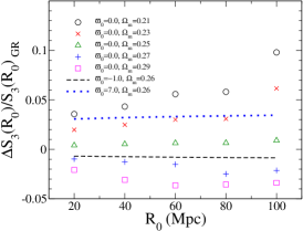
The smoothed skewness (106) cannot be written as a simple function of growth factors. It must be integrated over the 6 dimensional parameter space $\{\vec{k}_{1},\vec{k}_{2}\}$, which can be reduced to a 4 dimensional parameter space upon noting that the integrand in equation (108) does not explicitly depend on the azimuthal angles $\phi_{k_{1}}$ or $\phi_{k_{2}}$ so that we can replace those two integrations with a factor of $4\pi^{2}$. We use the same Monte Carlo integrator we used in Section IV. We present our results in Figure (8) as a change in skewness (relative to a WMAP 5-year maximum likelihood GR universe; see equation 102). While $\varpi_{0}$ retains the strong influence on $S_{3}$ observed in Figure 7, the effect of $\Omega_{m}$ on the shape of the power spectrum amplifies its influence, so that it is now very difficult to distinguish between a significant departure from general relativity and a minor shift in $\Omega_{m}$. We perform a similar calculation for $S_{4}(R_{0})$ in Section C.

Figure 8: We plot the smoothed skewness (106) as a function of scale $R_{0}$ for different values of $\varpi_{0}$ and $\Omega_{m}$. Results are presented (as in Figure 7) as a change in skewness relative to the WMAP 5-year maximum likelihood GR cosmology. While $\varpi_{0}$ retains the strong influence on $S_{3}$ observed in Figure 7, the effect of $\Omega_{m}$ on the shape of the power spectrum amplifies its influence, so thtat it is now very difficult to distinguish between a significant departure from general relativity and a minor shift in $\Omega_{m}$. The $1\sigma$ confidence interval reported by the WMAP 5-year team is $\Omega_{m}=0.26\pm 0.03$.

Appendix C Fourth order moments

The smoothed kurtosis $S_{4}(R_{0})$ of the overdensity distribution is the fourth order moment of the distribution averaged over a radius $R_{0}$, i.e.

$$S_{4}(R_{0})=\frac{\langle\delta_{R_{0}}(\vec{x})^{4}\rangle-3\langle\delta_{R_{0}}(\vec{x})^{2}\rangle^{2}}{\langle\delta_{R_{0}}(\vec{x})^{2}\rangle^{3}}.$$ (110)

In this section, we will show the effect of $\varpi\neq 0$ on $S_{4}(R_{0})$. While the effect is stronger than that found on the skewness in Section B, this is of little comfort because, as a higher order moment, the kurtosis is much harder to measure than the (already difficult) skewness. Also, we find that the effect of varying $\Omega_{m}$ is similarly amplified so that it would still be difficult to discern a large change in $\varpi_{0}$ from a small change in $\Omega_{m}$.

C.1 Third order equations of motion

Calculating the kurtosis requires first that we find the evolution of the third order perturbations $\{\phi^{(3)},\delta^{(3)},\vec{v}^{(3)}\}$. We do so in this section. For easy reference, we recall the first and second order solutions

$$\phi^{(1)} = f(\tau)\varphi(\vec{x})$$

$$\delta^{(1)} = D(\tau)\nabla^{2}\varphi$$

$$\vec{v}^{(1)} = -\dot{D}\vec{\nabla}\varphi(\vec{x})$$

$$\phi^{(2)} = \alpha(\tau)A(\vec{x})+\beta(\tau)B(\vec{x})$$

$$\delta^{(2)} = \mathcal{D}^{(a)}(\tau)\nabla^{2}A+\mathcal{D}^{(b)}(\tau)\nabla^{2}B$$

$$\vec{v}^{(2)} = (-\dot{\mathcal{D}}^{a}+D\dot{D})\vec{\nabla}A-\dot{\mathcal{D}}^{b}\vec{\nabla}B$$

$$\nabla^{2}A = \partial_{i}\left(\nabla^{2}\varphi\partial_{i}\varphi\right)$$

$$\nabla^{2}B = \partial_{ij}\left(\partial_{i}\varphi\partial_{j}\varphi\right).$$

The third-order part of equation (II) is

$$\ddot{\delta}^{(3)}+\mathcal{H}\dot{\delta}^{(3)} = (1+\varpi)\left(\partial_{i}\delta^{(2)}\partial_{i}\phi^{(1)}+\partial_{i}\delta^{(1)}\partial_{i}\phi^{(2)}\right)+\partial_{ij}\left[2v^{i(2)}v^{j(1)}+\delta^{(1)}v^{i(1)}v^{j(1)}\right]$$ (111)

$$+(1+\varpi)\big{(}\delta^{(1)}\nabla^{2}\phi^{(2)}+\delta^{(2)}\nabla^{2}\phi^{(1)}+\nabla^{2}\phi^{(3)}\big{)}.$$

Using the recipe outlined in Section II, we find

$$\phi^{(3)} = \sum_{i=1}^{7}F^{(i)}(\tau)\mathcal{G}^{(i)}(\vec{x})$$

$$\delta^{(3)} = \sum_{i=1}^{7}\mathcal{F}^{(i)}(\tau)\nabla^{2}\mathcal{G}^{(i)}(\vec{x})$$ (112)

where

$$\nabla^{2}\mathcal{G}^{(1)} = \partial_{i}\left[\partial_{i}\varphi\nabla^{2}A\right]$$

$$\nabla^{2}\mathcal{G}^{(2)} = \partial_{i}\left[\partial_{i}\varphi\nabla^{2}B\right]$$

$$\nabla^{2}\mathcal{G}^{(3)} = \partial_{i}\left[\nabla^{2}\varphi\partial_{i}A\right]$$

$$\nabla^{2}\mathcal{G}^{(4)} = \partial_{i}\left[\nabla^{2}\varphi\partial_{i}B\right]$$ (113)

$$\nabla^{2}\mathcal{G}^{(5)} = \partial_{ij}\left[\partial_{j}\varphi\partial_{i}A\right]$$

$$\nabla^{2}\mathcal{G}^{(6)} = \partial_{ij}\left[\partial_{j}\varphi\partial_{i}B\right]$$

$$\nabla^{2}\mathcal{G}^{(7)} = \partial_{ij}\left[\nabla^{2}\varphi\partial_{i}\varphi\partial_{j}\varphi\right].$$

The equations of motion for $F^{(i)}$ and $\mathcal{F}^{(i)}$ are

$$\ddot{F}^{(i)} = -\dot{F}^{(i)}\mathcal{H}(3+\varpi)-F^{(i)}\left[\mathcal{H}^{2}3(1+\varpi)(1-\Omega_{m})+\mathcal{H}\dot{\varpi}\right]+\frac{3}{2}\Omega_{m}\mathcal{H}^{2}S^{(3,i)}$$

$$\ddot{\mathcal{F}}^{(i)} = -\mathcal{H}\dot{\mathcal{F}}^{(i)}+(1+\varpi)F^{(i)}+S^{(3,i)}.$$

The right hand side of equation (111) gives

$$S^{(3,1)} = (1+\varpi)f\mathcal{D}^{(a)}$$

$$S^{(3,2)} = (1+\varpi)f\mathcal{D}^{(b)}$$

$$S^{(3,3)} = (1+\varpi)D\alpha$$

$$S^{(3,4)} = (1+\varpi)D\beta$$

$$S^{(3,5)} = -2\dot{D}(-\dot{\mathcal{D}}^{a}+\dot{D}D)$$

$$S^{(3,6)} = 2\dot{D}\dot{\mathcal{D}}^{b}$$

$$S^{(3,7)} = D\dot{D}^{2}.$$

C.2 The kurtosis

The numerator of equation (110) is equivalent to

$$\langle\delta_{R_{0}}(\vec{x})^{4}\rangle-3\langle\delta_{R_{0}}(\vec{x})^{2}\rangle^{2}=4\langle\delta^{(1)3}\delta^{(3)}\rangle+6\langle\delta^{(1)2}\delta^{(2)2}\rangle.$$

Using equation (112) and drawing an analogy with equation (108), we find that

$$\langle\delta^{(1)3}\delta^{(3)}\rangle = 4\int\frac{d^{3}k_{1}d^{3}k_{2}d^{3}k_{3}}{(2\pi)^{9}}\frac{P(k_{1})P(k_{2})P(k_{3})}{D^{3}}W_{1}W_{2}W_{3}W_{1+2+3}\sum_{i=1}^{7}\mathcal{F}^{(i)}\sum_{\text{perm}}\tilde{\mathcal{G}}^{(i)}(\vec{k}_{1},\vec{k}_{2},\vec{k}_{3})$$ (114)

where $\sum_{\text{perm}}\tilde{\mathcal{G}}^{(i)}=\tilde{\mathcal{G}}^{(i)}(\vec{k}_{1},\vec{k}_{2},\vec{k}_{3})+\tilde{\mathcal{G}}^{(i)}(\vec{k}_{1},\vec{k}_{3},\vec{k}_{2})+\dots$ and the $\tilde{\mathcal{G}}^{(i)}$ are the Fourier transforms of equations (113) with all factors of $\varphi$ artificially removed.

Similarly, the other part of the kurtosis reduces to

$$\langle\delta^{(1)2}\delta^{(2)2}\rangle = 6\int\frac{d^{3}k_{1}d^{3}k_{2}d^{3}k_{3}}{(2\pi)^{9}}\frac{P(k_{1})P(k_{2})P(k_{3})}{D^{4}}W_{1}W_{2}\sum_{\text{perm}}W_{3-1}W_{-3-2}\tilde{\mathcal{D}}(\vec{k}_{3},-\vec{k}_{1})\tilde{\mathcal{D}}(-\vec{k}_{3},-\vec{k}_{2})$$ (115)

$$\tilde{\mathcal{D}}(\vec{k}_{i},\vec{k}_{j}) = k_{i}^{2}k_{j}^{2}\Bigg{[}\mathcal{D}^{(a)}\left(1+\frac{\vec{k}_{i}\cdot\vec{k}_{j}}{k_{i}^{2}}\right)+\mathcal{D}^{(b)}\left(1+2\frac{\vec{k}_{i}\cdot\vec{k}_{j}}{k_{i}^{2}}+\frac{(\vec{k}_{i}\cdot\vec{k}_{j})^{2}}{k_{i}^{2}k_{j}^{2}}\right)\Bigg{]}.$$ (116)

In this case $\sum_{\text{perm}}W_{3-1}W_{-3-2}\tilde{\mathcal{D}}(\vec{k}_{3},-\vec{k}_{1})\tilde{\mathcal{D}}(-\vec{k}_{3},-\vec{k}_{2})$ has 8 terms, permuting over both the content of the two pairs of vectors

$$\tilde{\mathcal{D}}(\vec{k}_{3},-\vec{k}_{1})\tilde{\mathcal{D}}(-\vec{k}_{3},-\vec{k}_{2})\rightarrow\tilde{\mathcal{D}}(\vec{k}_{3},-\vec{k}_{2})\tilde{\mathcal{D}}(-\vec{k}_{3},-\vec{k}_{1})\text{, etc.}$$

and permuting over the vectors’ orders within the pairs

$$\tilde{\mathcal{D}}(\vec{k}_{3},-\vec{k}_{1})\tilde{\mathcal{D}}(-\vec{k}_{3},-\vec{k}_{2})\rightarrow\tilde{\mathcal{D}}(-\vec{k}_{1},\vec{k}_{3})\tilde{\mathcal{D}}(-\vec{k}_{2},-\vec{k}_{3})\text{, etc.}$$

Note also that $\vec{k}_{3}$ is always positive in the first pair and negative in the second. $\vec{k}_{1}$ and $\vec{k}_{2}$ are always negative. These minus signs are acquired from the delta function in

$$\langle\tilde{\delta}^{(1)}(\vec{k}_{i})\tilde{\delta}^{(1)}(\vec{k}_{j})\rangle=P(k_{i})\delta^{3}_{D}(\vec{k}_{i}+\vec{k}_{j}).$$

Figure 9 recreates Figure 8 for the smoothed kurtosis. Again we find that it is nearly impossible to distinguish a large change in $\varpi_{0}$ from a small change in $\Omega_{m}$.

Figure 9: We plot the smoothed kurtosis (110) as a function of scale $R_{0}$ for different values of $\varpi_{0}$ and $\Omega_{m}$. Results are presented (as in Figure 3) as a change in kurtosis relative to the WMAP 5-year maximum likelihood GR cosmology. The $1\sigma$ confidence interval reported by the WMAP 5-year team is $\Omega_{m}=0.26\pm 0.03$.