From Incoherence to Synchronicity in the Network Kuramoto model

Abstract

We study the synchronisation properties of the Kuramoto model of coupled phase oscillators on a general network. Here we distinguish the ability of such a system to self-synchronise from the stability of this behaviour. While self-synchronisation is a consequence of genuine non-perturbative dynamics, the stability in dynamical systems is usually accessible by fluctuations about a fixed point, here taken to be the synchronised solution. We examine this problem in terms of modes of the graph Laplacian, by which the absolute Lyapunov stability of the synchronised fixed point is readily demonstrated. Departures from stability are seen to arise at the next order in fluctuations where the dynamical equations resemble those for species population models, the logistic and Lotka-Volterra equations. Methods from these systems are exploited to analytically derive new critical couplings signalling deviation from classical stability. We observe in some cases an intermediate regime of behaviour, between incoherence and synchronisation, where system wide periodic behaviours are exhibited. We discuss these results in light of simulations.

I Introduction

The study of the ability of systems to achieve self-synchronisation – coherent behaviour purely through the mutual interactions of many components – is a major theme in complex systems science. The phenomenon arises in many contexts, from ecology, biology, physics to social systems. In our case the understanding of self-synchronisation through complex networks in command and control organisations is a major goal Kall08 . Notable early work on collective synchronisation includes that of Wiener Wie58 and Winfree Win67 . Kuramoto’s elegantly simple model Kur84 , upon which we focus, encapsulates much of the richness expected in self-synchronising systems. Strogatz Stro00 gives a short elegant introduction while Acebrón et al. Ace05 provide a more thorough review.

The Kuramoto model involves one-dimensional phase oscillators described by angles $\theta_{i}$ coupled on a network described by an undirected graph $G$ of size $N$ and is given by the first order differential equation

$$\dot{\theta}_{i}=\omega_{i}-\frac{K}{N}\sum_{j}A_{ij}\sin(\theta_{i}-\theta_{j}).$$ (1)

Here $A_{ij}$ is the adjacency matrix encoding the graph structure, $\omega_{i}$ are intrinsic frequencies of the oscillators, usually drawn from some statistical distribution and $K$ is a uniform coupling controlling the degree to which adjacent oscillators must mutually adjust with respect to each other. At zero coupling the system obviously behaves incoherently with each oscillator moving in simple harmonic motion according to its intrinsic frequency. Increasing the coupling enables the population to eventually break into synchrony, with some of the oscillators locking into a single core that moves with harmonic motion according to the frequency average over the whole oscillator ensemble. For the case of an infinite, complete graph and symmetric and unimodal distribution of intrinsic frequencies Kuramoto was able to derive an exact analytic expression for the critical coupling $K_{c}$ at which synchrony breaks out

$$K_{c}={{2}\over{\pi g(0)}}$$ (2)

where $g(0)$ is the central value of the distribution $g$ from which the intrinsic frequencies of the individual oscillators are selected.

On a general network no equivalent analytic expression for Kuramoto’s critical coupling has been derived. This paper shall take some steps in that direction. While analytic methods have been applied to mean-field versions of the model, such as in Ich04 , numerical simulations have delivered insights into the pattern of synchronisation for the complete form of the Kuramoto model on finite general networks. For random graphs (such as Erdös-Renyi) it is observed by Gomez07 that, as the coupling is increased, synchrony first develops locally on separate hubs which finally merge into a single locked system after the coupling has crossed a final threshold. The same authors find that for “scale-free” networks AlbBar02 the synchrony develops at one point in the graph and then extends to the whole graph as coupling is increased. For the Watts-Strogatz “small world” network WattsStrog98 synchronisation occurs even for small rewiring probability Hong02 . Such work already shows that quite specific graph substructures play a subtle role in the transient towards synchronisation, both in manifesting local synchronisation and, possibly, stimulating it in other parts of the network. Further insight is offered by Arenas et al. Aren06 who find evidence that the relevant sub-structures are the modes of the graph Laplacian, an object that is ubiquitous in network coupled dynamical systems Chung97 ; Boll98 . Indeed, for graphs with hierarchical community structure the order in which substructures settle into synchronisation is according to the Laplacian eigenvalue, with the largest mode synchronising first and the smallest stabilising last Aren06 . A more thorough review of numerical studies is provided by Dor08 .

At the heart of it, synchronisation and its stability are two separate phenomena in such systems. These aspects are often confused in the literature, so that, in some cases, stability criteria (derived perturbatively) are treated as synonymous with synchronisability (a deeply non-perturbative phenomenon). Intuitively, the distinction can be appreciated from the perspective of a potential energy landscape for the entire system. The evolution of the system from some random initial condition to complete synchronisation can be visualised as a walk through this landscape, from the “edges” (incoherent behaviour) to the “centre” (coherence) through a typically rough intermediate landscape. Synchronisation is the means by which the system passes through the bulk of the rough landscape close to the centre. Stability is a local property of the vicinity of the centre. In the vicinity of the synchronised solution, for stability, perturbative methods are applicable. This is where this paper will focus and provide new analytical insights. The mechanism for the system finding its way through the landscape is a genuine nonperturbative problem for which analytic methods are lacking in the finite general network case though numerical studies have provided significant insights. This paper will offer an hypothesis, building on the insights from the existing numerical studies.

While most stability studies are performed for the infinite network case using the formalism of probability densities Mir05 , in the finite case there is little that has been published specifically for the Kuramoto model. We suspect that this is because many researchers may have implicitly appreciated that the synchronised solution is Lyapunov stable and decided that there was little more to be said. We shall review this aspect in terms of eigenmodes of the graph Laplacian. In these terms, the synchronised solution turns out to be just the zero mode of the Laplacian while the normal mode fluctuations, to first order, exponentially decay to zero consistent with the Lyapunov stability criterion. More generally, in this framework, we make the observation that the synchronisation problem can be reframed as a population competition dynamics. The question then becomes: how do the normal mode interactions lead to an “extinction” of these modes? We answer this question by extending considerations to second order in the lowest lying Laplacian normal mode fluctuations and extracting equations more commonly seen in species-population models. Though we argue that all the low-lying Laplacian normal modes are significant in the generation of instabilities in the system, we shall study analytically the role, respectively, of one and two of the lowest-lying Laplacian normal modes in generating instabilities of the synchronised fixed point. The lowest Laplacian normal mode, whose relationship to measuring connectivity in a network was noted by Fiedler Fied73 , has often been argued to be relevant to the problem, as we shall review below. In our analysis we show that the dynamics of a single lowest mode are governed by a modification of the logistic equation while for two lowest modes a form of Lotka-Volterra equations are obtained. Though, for many complex networks, these are rather artificial cases, we derive critical couplings here to illustrate the types of dynamics that can occur. Indeed, we identify in some cases a previously (to our knowledge) unnoticed regime lying between incoherence and coherence, a type of “edge-of-chaos” patterned dynamics. We provide support for this by showing examples of simulations for this system.

The paper is structured as follows. In the next section we recast the Kuramoto model in terms of modes of the graph Laplacian and review the Lyapunov stability of the system. Then we develop the problem to second order in fluctuations and study several cases for the structure of the lowest normal modes of the Laplacian. We derive a number of critical couplings for several special cases. We subsequently analyse the behaviour of an order parameter for synchronisation of the system in these terms and discuss this in light of simulations. The final section will discuss our insights into the general mechanism for synchronisation and the subtleties of generalising these results to the complete infinite graph, originally studied by Kuramoto.

II Laplacian eigenmodes and stability

II.1 Comparison of Kuramoto model with other coupled dynamical models

Let us begin by contrasting the Kuramoto model, Eq.(1), with another class of coupled dynamical system which has been studied intensively for some time:

$$\dot{\phi_{i}}=f(\phi_{i})+\sigma\sum_{j}A_{ij}\left[g(\phi_{j})-g(\phi_{i})\right].$$

We shall consistently use the graph (or combinatorial) Laplacian Chung97 ; Boll98 ,

$$L_{ij}=d_{i}\delta_{ij}-A_{ij},$$ (3)

with $d_{i}$ is the degree of node $i$. The spectrum of the Laplacian is positive semi-definite, so that eigenvalues can be ordered from smallest to largest:

$$0=\lambda_{0}\leq\lambda_{1}\leq\dots\leq\lambda_{N-1}.$$ (4)

(In some of the literature the numbering of modes starts at one and not zero.) In these terms, the dynamical system can be rewritten

$$\dot{\phi_{i}}=f(\phi_{i})-\sigma\sum_{j}L_{ij}g(\phi_{j}).$$ (5)

Synchronisation is represented by fixed point solutions $\phi_{i}=s$ of Eq.(5). Fluctuations $\eta_{i}$ about $s$ satisfy then

$$\dot{\eta}_{i}=f^{\prime}(s)\eta_{i}-\sigma g^{\prime}(s)\sum_{j}L_{ij}\eta_{j}.$$

Going to a basis of eigenmodes for the fluctuations leads to a criterion for stability of the synchronised solution:

$$\int_{0}^{t}d\tau\left[f^{\prime}(s(\tau))-\sigma g^{\prime}(s(\tau))\lambda_{r}\right]<0$$

for all Laplacian modes $r$. This “master stability equation” was derived by Pecora and Carroll Pec98 . Many others have exploited this approach to study a variety of networks, for example various . Significantly, we see that, depending on the network and the nature of the functions $f$ and $g$, there may be directions in Laplacian mode space for which this condition is not satisfied. Therefore, within a first order perturbation calculation we can determine a condition for which synchronisation can exist and is stable. It is tempting on this basis to see synchronisation purely through the lens of Lyapunov stability.

Unfortunately, the Kuramoto model Eq.(1) is very different from this system. This is because the interaction in the Kuramoto model is a function of differences rather than a difference of functions. Practically, it means that the dynamics are not automatically diagonalised in the Laplacian eigenmode basis. However, small fluctuations about the synchronisation point can be diagonalised in terms of the Laplacian.

II.2 Representation in Laplacian Basis

Before diving into this, let us present some more details on the Laplacian. The degeneracy of zero eigenmodes of the Laplacian corresponds to the number of disconnected components of the graph. We shall concern ourselves with connected graphs, so there will be a single zero mode. The corresponding zero mode eigenvector, within a system of orthonormal eigenvectors, is

$$\nu^{(0)T} = \frac{1}{\sqrt{N}}(1,1,\dots,1),$$ (6)

$$L\nu^{(r)} = \lambda_{r}\nu^{(r)},$$

$$\nu^{(r)}\cdot\nu^{(s)} = \delta_{rs}.$$

The first nonzero eigenmode, here corresponding to $\lambda_{1}$, is called the Fiedler with the eigenvalue itself known as the algebraic connectivity Fied73 . The eigenmode itself is used in other contexts as a measure of network fragility Ding01 . Though we are dealing with unoriented graphs, it is convenient to rewrite the Laplacian in terms of a signed incidence matrix $B$ as follows. Let links, which may be assigned an arbitrary direction for this purpose, be labelled by the index $a$. Matrix elements of $B$ are $B_{ia}$ where

$$B_{ia}=+1,0,-1$$

according to whether link $a$ is incoming to, not connected with or outgoing from node $i$. The Laplacian is then given by

$$L=BB^{T}.$$

The signed incidence matrix has deep mathematical properties, but one role that it plays is to transform between objects respectively in the node and link spaces, including the eigenvectors:

$$e^{(r)} = B^{T}\nu^{(r)}$$ (7)

$$e^{(r)}\cdot e^{(s)} = \lambda_{r}\delta_{rs}.$$

In terms of the original eigenvectors we can expand a phase angle of the Kuramoto model in the Laplacian basis

$$\theta_{i}(t)=\sum_{r=0}\alpha_{r}(t)\nu^{(r)}_{i}.$$

Inserting this in the equation of motion Eq.(1) we arrive at equations for the components:

$$\alpha_{0} = \sqrt{N}\bar{\omega}t$$ (8)

$$\dot{\alpha_{r}}(t) = \omega^{(r)}-\sigma\sum_{a}e^{(r)}_{a}\sin\left(\sum_{s>0}e^{(s)}_{a}\alpha_{s}(t)\right);$$ (9)

$$r\neq 0$$

where from this point we summarise the coupling as $\sigma=K/N$. Also implicit in Eq.(9) is that we treat the $\omega_{i}$ as an $N$-dimensional vector, with $\bar{\omega}$ the average over the distribution and

$$\omega^{(r)}=\omega\cdot\nu^{(r)}$$

represents the projection of the vector of frequencies $\omega_{i}$ onto the $r$-th Laplacian mode.

II.3 Interpretation of normal mode dynamics

From Eq.(8), we see that the zero mode is just the synchronised mode and that it completely decouples from the normal modes. Therefore, in terms of Laplacian modes there is always a component moving harmonically with the average frequency. Posed this way, the concern ceases to be how synchronisation is generated but how the normal mode dynamics in Eq.(9) are suppressed. Indeed, we can reformulate the problem in the language of another classical complex systems problem: that of inter/intra-species population dynamics. Recall that in this context, populations can grow, die out and compete with others in predator-prey relationships. Within such interactions, oscillating population numbers for co-existing species can occur.

In this language, then, pure oscillator synchronisation is identical to normal eigenmode population extinction and complete oscillator incoherence is identical to multiple species normal eigenmode population co-existence. Later in the paper, we shall refine this relationship further and identify specific cases of behaviours according to interacting population dynamics manifested here in the competing Laplacian normal eigenmodes.

II.4 Lyapunov Stability

We can now review standard stability arguments. Let the system be close to complete synchronisation, now characterised by the zero mode,

$$\theta_{i}(t)\approx\alpha_{0}(t)\nu_{i}^{(0)}+{\rm{small}},$$

with small fluctuations being some superposition of the normal modes. Expanding the interaction term for small normal modes to leading order, we obtain

$$\dot{\alpha_{r}}(t)=\omega^{(r)}-\sigma\lambda_{r}\alpha_{r}(t);r\neq 0.$$ (10)

The solution to this is just

$$\alpha_{r}(t)={{\omega^{(r)}}\over{\sigma\lambda_{r}}}(1-e^{-\sigma\lambda_{r}t})+\alpha_{r}(0)e^{-\sigma\lambda_{r}t}.$$ (11)

Part of this equation was obtained by Arenas et al. Aren06 , who only presented the second term as their focus was on the hierarchy of suppression of modes. This supports the idea that the sequence of clusters achieving synchronisation occurs sequentially in time through the hierarchy of eigenvalues in Eq.(4). Specifically, fluctuations in the highest mode of the Laplacian, corresponding to $\lambda_{N-1}$, are suppressed most quickly; the last mode to be suppressed is the lowest non-zero mode, the Fiedler with eigenvalue $\lambda_{1}$. If suppression is achieved, the modes become constant

$$\alpha_{r}^{(\infty)}={{\omega^{(r)}}\over{\sigma\lambda_{r}}}.$$ (12)

Note that the complete graph has a completely degenerate Laplacian normal mode spectrum: $\lambda_{i}=N,\ i=1,\dots,N-1$. The implications of this degeneracy are discussed in the final section. We observe in Eq.(12) that the regime of applicability of synchronisation is characterised by small $\alpha_{r}^{(\infty)}$, namely

$$\sigma>{{\omega^{(r)}}\over{\lambda_{r}}}$$ (13)

which can be seen as a (very) weak bound on critical values of the coupling such that synchronisation can occur. However, this bound does not indicate what types of transitions can occur.

We see that in the vicinity of the synchronized solution the system is Lyapunov stable in all directions in Laplacian mode space: the Lyapunov exponents are exactly the Laplacian eigenvalues multiplied by the coupling so that there are no regimes of coupling or structure whereby they may change sign. This has also been observed by Jadbabaie et al. Jad04 using different methods. These authors also derive certain bounds on the coupling, related to our bound Eq.(13), which, however, do not readily return the special case derived by Kuramoto for the infinite complete graph. We suspect this is a consequence of the absolute Lyapunov stability of the system and return to this at the end of the next section.

III Second order approximations

In the following we extend the above approximation to next order in the Taylor expansion of the interaction in the equations of motion and making certain simplifying assumptions on the structure of the lowest modes of the Laplacian. Specifically, we expand the sine in Eq.(9) out to the cubic term, $\sin x=x-x^{3}/6$. This means that our approximations are valid for values of $\alpha_{r}$ larger than considered in standard stability analysis thus far, out to values of $x\sim\pi/2>1$. Furthermore we shall assume sufficient time to have elapsed in the running of the system dynamics so that most Laplacian modes are suppressed to $\alpha_{r}^{(\infty)}$. The exception to this will be a number of the lowest modes which will be taken to be dynamical. In other words, we exploit the observation in numerical simulations that modes with small Laplacian eigenvalue synchronise later, though we make no assumptions about the order of synchronisation of the higher modes. We shall now explore the impact of these few small eigenvalue dynamical modes on stability.

III.1 One dynamical mode

III.1.1 Exact solutions

In this case we have a single mode that remains time-dependent, namely that corresponding to the Fiedler, $\alpha_{1}(t)$. All other modes $r>1$ assume their steady-state values Eq.(12). We assume in this part that there is no degeneracy for $\lambda_{1}$, which will be relaxed in the next section. Thus we separate the mode sum in Eq.(9) into two parts,

$$\sum_{s>0}e^{(s)}_{a}\alpha_{s}(t)=e^{(1)}_{a}\alpha_{1}(t)+\sum_{s>1}e^{(s)}_{a}\alpha_{s}^{(\infty)},$$ (14)

and insert this into Eq.(9). Within the expansion of the sine we drop all terms cubic in any given mode and those quadratic in the constant modes $\alpha_{s}^{(\infty)}$. To this order then we extract the equation

$$\dot{\alpha_{1}}(t)=\omega^{(1)}-\sigma\lambda_{1}\alpha_{1}(t)+\sigma x_{1}\alpha_{1}(t)^{2},$$ (15)

where we define constants summarising the dynamical and structural content of the system

$$x_{r} = \sum_{s>1}{c_{rs}{\omega^{(s)}\over{2\sigma\lambda_{s}}}},$$

$$c_{rs} = \sum_{a}(e^{(r)}_{a})^{3}e^{(s)}_{a},\ s\neq r.$$

Eq.(15) is a variation on the well-known logistic equation. We further introduce the notation (the first being the discriminant of a quadratic equation):

$$\Delta_{1} = \sigma^{2}\lambda_{1}^{2}-4\sigma\omega^{(1)}x_{1},$$

$$P_{1}(0) = {{2\sigma x_{1}\alpha_{1}(0)-(\sigma\lambda_{1}+\sqrt{\Delta_{1}})}\over{2\sigma x_{1}\alpha_{1}(0)-(\sigma\lambda_{1}-\sqrt{\Delta_{1}})}}.$$

The solution to Eq.(15) depends on the sign of the discriminant $\Delta_{1}$. When the coupling strength $\sigma$ is varied, say, from large to down small values the discriminant changes sign, from positive, through zero, zero to negative values.

For large $\sigma\lambda_{1}$ the solution is

$$\alpha_{1}(t)={{(\sigma\lambda_{1}+\sqrt{\Delta_{1}})-(\sigma\lambda_{1}-\sqrt{\Delta_{1}})P_{1}(0)e^{\sqrt{\Delta_{1}}t}}\over{2\sigma x_{1}(1-P_{1}(0)e^{\sqrt{\Delta_{1}}t})}}.$$ (16)

This will return the first order solution when $\lambda_{1}\ll\lambda_{2}$. Then $x_{1}\approx 0$ and the right hand side of Eq.(16) can be expanded for small $x_{1}$ giving Eq.(11). This reflects the behaviour that the solution to Eq.(15) starts from the initial condition and then is exponentially suppressed to the constant value Eq.(12). There can occur points where, at some fixed time, the denominator of Eq.(16) vanishes; the solution shoots to negative infinity and then returns to stabilise at the constant value Eq.(12).

When the discriminant is negative the solution takes the form

$$\alpha_{1}(t)=\frac{1}{2\sigma x_{1}}\times$$

$$\left[\sigma\lambda_{1}+\tan\left(\arctan(2\sigma x_{1}\alpha_{1}(0)-\sigma\lambda_{1})+\sqrt{-\Delta}_{1}\frac{t}{2}\right)\right].$$

(17)

This displays both “accidental” divergent behaviour, when the argument of the tangent becomes $\pi/2$ and, more significantly, periodicity in time. In this regime then, the normal modes are dominated by a limit cycle and the lowest Laplacian mode never converges to steady state.

Therefore the condition $\Delta_{1}=0$ separates two distinct regimes of behaviour: for $\Delta_{1}<0$ complete synchronisation is not attained while for $\Delta_{1}>0$ convergence to the fixed point occurs. We can thus extract a critical coupling:

$$\sigma_{c}=2\sum_{s>1}{{\omega^{(1)}c_{1s}\omega^{(s)}}\over{\lambda_{1}^{2}\lambda_{s}}}.$$ (18)

This reflects a genuine point at which the dynamics changes distinctly in character in contrast to the bound Eq.(13) derived purely within a first order stability analysis.

III.1.2 Equilibrium analysis

Even though we have analytical solutions here it is worth reinforcing these results by looking at the equilibrium dynamics in this regime. Setting $\dot{\alpha_{1}}=0$ in Eq.(15), two solutions result:

$$\alpha_{1}^{\pm}={{\sigma\lambda_{1}\mp\sqrt{\Delta_{1}}}\over{2\sigma x_{1}}}.$$

In fact these match on to the analytical solution for $t\rightarrow\pm\infty$ of Eq.(16):

$$\alpha_{1}^{\pm}=\lim_{t\rightarrow\pm\infty}\alpha_{1}(t).$$

As a preview to the next section, let us examine stability about these equilibria. Inserting

$$\alpha_{1}=\alpha_{1}^{\pm}+\chi^{\pm}$$

into Eq.(15) we obtain the order $\chi$ equation

$$\dot{\chi} = (2\sigma x_{1}\alpha^{\pm}-\sigma\lambda_{1})\chi^{\pm}$$

$$= \mp\sqrt{\Delta_{1}}\chi^{\pm}$$

The solution manifests a Lyapunov-like exponent:

$$\chi^{\pm}=\chi^{\pm}(0)e^{\mp\sqrt{\Delta_{1}}t}$$

Again, we are only interested in the $t\rightarrow\infty$ behaviour, namely in $\chi^{+}$. Examining the strong coupling case $\sigma>1/\lambda_{1}$ we obtain

$$\alpha_{1}^{+} \rightarrow {{\omega^{(1)}}\over{\sigma\lambda_{1}}}$$ (19)

$$\alpha_{1}^{-} \rightarrow {{\lambda_{1}}\over{x_{1}}}-{{\omega^{(1)}}\over{\sigma\lambda_{1}}}.$$ (20)

Thus, for $t\rightarrow\infty$, Eq.(19) coincides with the original lowest order steady state result, Eq.(12).

We now appreciate the two regimes of behaviour seen in Eqs.(16,17) in another light: $\Delta_{1}>0$ manifests stability, namely convergence as $t\rightarrow\infty$ to the equilibrium fixed point while $\Delta_{1}<0$ gives an imaginary phase, namely a limit cycle.

III.2 Two dynamical modes

Let us consider initially now the lowest two normal modes, $\alpha_{1}$ and $\alpha_{2}$, to be dynamical with all others having reached steady state. Initially we consider all terms linear in the constant modes $\alpha_{r}^{(\infty)}$ but up to quadratic in the dynamical modes $\alpha_{s}(t)$ ($s=1,2$). The full system to this order has the form

$$\dot{\alpha_{1}}(t) = \omega^{(1)}-\sigma\lambda_{1}\alpha_{1}(t)+\sigma\alpha_{1}^{2}X_{1}+\sigma\alpha_{1}(t)\alpha_{2}(t)Y_{1}$$

$$+\sigma\alpha_{2}(t)^{2}Z_{1}$$

$$\dot{\alpha_{2}}(t) = \omega^{(2)}-\sigma\lambda_{2}\alpha_{1}(t)+\sigma\alpha_{2}^{2}X_{2}+\sigma\alpha_{1}(t)\alpha_{2}(t)Y_{2}$$ (21)

$$+\sigma\alpha_{1}(t)^{2}Z_{2},$$

with a set of dynamical and structural constants

$$X_{r} \equiv \sum_{s>2}C_{rs}{{\omega^{(s)}\over{2\sigma\lambda_{s}}}}$$

$$Y_{r} \equiv \sum_{s>2}D_{rs}{{\omega^{(s)}\over{\sigma\lambda_{s}}}}$$

$$Z_{r} \equiv \sum_{s>2}E_{rs}{{\omega^{(s)}\over{2\sigma\lambda_{s}}}}$$

$$C_{rs} \equiv \sum_{a}(e^{(r)}_{a})^{3}e^{(s)}_{a}$$

$$D_{1s} \equiv \sum_{a}(e^{(1)}_{a})^{2}e^{(2)}_{a}e^{(s)}_{a}$$

$$E_{1s} \equiv \sum_{a}e^{(1)}_{a}(e^{(2)}_{a})^{2}e^{(s)}_{a}$$

$$D_{2s} = E_{1s}$$

$$E_{2s} = D_{1s}$$

by analogy with $x_{r}$ and $c_{rs}$ for the one-mode case.

Eqs.(21) are not amenable to analytic solution. However, analogously to the analysis of Sect.III.1.2, the equilibria and their stability are open to analysis (as is standard in predator-prey models). In other words, the intention is to study the case where $\dot{\alpha_{r}}=0$. Denoting such solutions to Eqs.(21) by $\alpha_{r}^{(u)}$, where $u$ represents some label for the different possible solutions, we then examine fluctations $\chi^{(u)}_{r}$ about these, namely solutions of the form $\alpha_{r}=\alpha_{r}^{(u)}+\chi_{r}^{(u)}$ keeping only terms of order $\chi$. The system Eqs.(21) with LHS set to zero is soluble however the solutions are extremely lengthy and cataloging the type of behaviours that can occur is difficult, though we should expect the full range of dynamical possibilities: stability, limit cycles, tori and instability. To illustrate this we consider a further truncation of the system, where only cross-interactions are kept. We comment later on the possible generality of our insights from this analysis.

III.2.1 Cross-interactions only, non-degenerate case

Treating the case that $\lambda_{1}\neq\lambda_{2}$, in the first instance, we are down to the coupled equations:

$$\dot{\alpha_{1}}(t) = \omega^{(1)}-\sigma\lambda_{1}\alpha_{1}(t)+\sigma\alpha_{1}(t)\alpha_{2}(t)Y_{1}$$

$$\dot{\alpha_{2}}(t) = \omega^{(2)}-\sigma\lambda_{2}\alpha_{1}(t)+\sigma\alpha_{1}(t)\alpha_{2}(t)Y_{2},$$ (22)

Apart from the first term, we recognise in Eqs.(22) the two dimensional Lotka-Volterra system for predator-prey dynamics Kap95 . That we have arrived at the next step in generalisation of population models after the logistic equation is consistent with our picture of the normal mode dynamics.

The solutions of Eqs.(22) with $\dot{\alpha}_{1}=\dot{\alpha}_{2}=0$ are compactly represented by introducing a new discriminant:

$$\Delta_{2}=(\sigma\lambda_{1}\lambda_{2}-(\omega^{(1)}Y_{2}-\omega^{(2)}Y_{1}))^{2}-4\sigma\lambda_{1}\lambda_{2}\omega^{(2)}Y_{1}.$$

Eqs.(22) exhibit two equilibria:

$$\alpha_{1}^{(\pm)} = {{\sigma\lambda_{1}\lambda_{2}+(\omega^{(1)}Y_{2}-\omega^{(2)}Y_{1})\mp\sqrt{\Delta_{2}}}\over{2\sigma\lambda_{1}X_{2}}}$$

$$\alpha_{2}^{(\pm)} = {{\sigma\lambda_{1}\lambda_{2}-(\omega^{(1)}Y_{2}-\omega^{(2)}Y_{1})\mp\sqrt{\Delta_{2}}}\over{2\sigma\lambda_{2}Y_{1}}}.$$ (23)

We consider now the fluctuations $\chi_{r}^{(u)}$ about these solutions by insertion into Eq.(22). We arrive at a fluctuation matrix whose eigenvalues give Lyapunov exponents for the equilibria Eqs.(23) which have the form

$$l_{1}^{(\pm)} = -{1\over{4\lambda_{1}\lambda_{2}}}\left(\sqrt{(A\pm B)^{2}\mp C}\pm(A\pm B)\right)$$

$$l_{2}^{(\pm)} = +{1\over{4\lambda_{1}\lambda_{2}}}\left(\sqrt{(A\pm B)^{2}\mp C}\mp(A\pm B)\right)$$ (24)

with

$$A = (\lambda_{1}+\lambda_{2})\sqrt{\Delta_{2}}$$

$$B = \sigma\lambda_{1}\lambda_{2}(\lambda_{1}+\lambda_{2})$$ (25)

$$-(\lambda_{2}-\lambda_{1})(\omega^{(1)}Y_{2}-\omega^{(2)}Y_{1})$$

$$C = 16\sigma\lambda_{1}^{2}\lambda_{2}^{2}\sqrt{\Delta_{2}}.$$

To get a handle on the equilibria in the absence of explicit analytic solutions it is worth examining first the strong coupling limit $\sigma>1/\lambda_{r}$. For the equilibria we obtain from Eqs.(23)

$$\alpha_{1}^{(+)} \rightarrow {{\omega^{(1)}}\over{\sigma\lambda_{1}}}$$

$$\alpha_{2}^{(+)} \rightarrow {{\omega^{(2)}}\over{\sigma\lambda_{2}}}$$

$$\alpha_{1}^{(-)} \rightarrow {{\lambda_{2}}\over{Y_{2}}}-{{\omega^{(2)}Y_{1}}\over{\sigma\lambda_{1}Y_{2}}}$$

$$\alpha_{2}^{(-)} \rightarrow {{\lambda_{1}}\over{Y_{1}}}-{{\omega^{(1)}Y_{2}}\over{\sigma\lambda_{2}Y_{1}}}$$

while the Lyapunov exponents Eqs.(24) give:

$$l_{1}^{(+)} \rightarrow -\sigma\lambda_{1}$$

$$l_{2}^{(+)} \rightarrow -\sigma\lambda_{2}$$

$$l_{1}^{(-)} \rightarrow -\sigma\sqrt{\lambda_{1}\lambda_{2}}$$

$$l_{2}^{(-)} \rightarrow +\sigma\sqrt{\lambda_{1}\lambda_{2}}.$$

We recognise then that $\alpha_{r}^{(+)}$ converge to the $t\rightarrow\infty$ form of the lowest order solutions. Our concern being with $t>0$ we therefore discard the solutions $\alpha_{r}^{(-)}$.

Noting that $A,C\geq 0$, we test the possible signs of the exponents in Eqs.(24). Consider, firstly, the case of the discriminant $\Delta_{2}>0$. Then it is straightforward to derive the following cases:

$$A+B>0 \Rightarrow l_{1}^{(+)}<0,\ l_{2}^{(+)}<0$$

$$A+B<0 \Rightarrow l_{1}^{(+)}>0{\rm{\ or\ complex}},\ l_{2}^{(+)}>0{\rm{\ or\ complex}}.$$

The complex values occur when $(A+B)^{2}<C$. Therefore, for $\Delta_{2}>0$, $\alpha_{1}$ and $\alpha_{2}$ will either be both stable or both display limit cycles. In the latter case, there can be real parts with positive sign in $l_{2}^{(+)}$ of Eqs.(24), indicating instability. We shall illustrate this in the simpler degenerate case below.

More interestingly, there is a precise coincidence between the “critical point”, given by $\Delta_{2}=0$, and an “edge-of-chaos” regime defined by vanishing Lyapunov exponents, $l_{2}^{(1)}=l_{2}^{(2)}=0$. The boundaries of this regime are governed by the two solutions to $\Delta_{2}=0$:

$$\sigma_{\pm}={1\over{\lambda_{1}\lambda_{2}}}(\omega^{(1)}Y_{2}+\omega^{(2)}Y_{1}\pm 2\sqrt{\omega^{(1)}\omega^{(2)}Y_{1}Y_{2}}).$$

Evidently $\sigma_{-}<\sigma_{+}$ and the two values indicate sign changes in $\Delta_{2}$: positive for $\sigma<\sigma_{-}$ and $\sigma>\sigma_{+}$ and negative for $\sigma_{-}<\sigma<\sigma_{+}$. Noting that at $\sigma=0$ we have $\Delta_{2}=(\omega^{(1)}Y_{2}-\omega^{(2)}Y_{1})^{2}>0$ then either both critical points, $\sigma_{\pm}$, are positive or both negative (and therefore unphysical as we consider only locally attractive interactions): if one critical point appears then there will be a second.

We conclude therefore that between incoherence for $\sigma\approx 0$ and coherence for $\sigma\gg 1/\lambda_{r}$ there will be an intermediate regime characterised by oscillatory behaviour whose frequency is not related to any individual oscillator but to the collective behaviour of the low-lying graph Laplacian modes.

III.2.2 Degenerate case

In the case that two lowest Laplacian eigenvalues are equal, $\lambda_{1}=\lambda_{2}$, a further simplification occurs. The Lyapunov exponents relevant for $t>0$ turn out to be:

$$l_{1}^{(+)} = -{1\over{2\lambda_{1}}}\left[|\sqrt{\Delta_{2}}-\sigma\lambda_{1}^{2}|+(\sqrt{\Delta_{2}}+\sigma\lambda_{1}^{2})\right]$$

$$l_{2}^{(+)} = {1\over{2\lambda_{1}}}\left[|\sqrt{\Delta_{2}}-\sigma\lambda_{1}^{2}|-(\sqrt{\Delta_{2}}+\sigma\lambda_{1}^{2})\right].$$

Consider firstly the case of $\Delta_{2}>0$. For $\sqrt{\Delta_{2}}>\sigma\lambda_{1}^{2}$ we have:

$$l_{1}^{(+)} = -{{\sqrt{\Delta_{2}}}\over{\lambda_{1}}}$$

$$l_{2}^{(+)} = -\sigma\lambda_{1}.$$

On the other hand, for $\sqrt{\Delta_{2}}<\sigma\lambda_{1}^{2}$ the exponents swap.

When the discriminant is negative we must take care with the modulus. Writing

$$\sqrt{\Delta_{2}}=i\sqrt{|\Delta_{2}|}$$

for this case, we have

$$|\sqrt{\Delta_{2}}-\sigma\lambda_{1}^{2}| = |\sigma\lambda_{1}^{2}-i\sqrt{|\Delta_{2}|}|$$

$$= \sqrt{|\Delta_{2}|+\sigma^{2}\lambda_{1}^{4}}.$$

Thus

$$l_{1}^{(+)} = -{1\over{2\lambda_{1}}}\left[\sqrt{|\Delta_{2}|+\sigma^{2}\lambda_{1}^{4}}+\sigma\lambda_{1}^{2}+i\sqrt{|\Delta_{2}|}\right]$$

$$l_{2}^{(+)} = {1\over{2\lambda_{1}}}\left[\sqrt{|\Delta_{2}|+\sigma^{2}\lambda_{1}^{4}}-\sigma\lambda_{1}^{2}-i\sqrt{|\Delta_{2}|}\right].$$

The fixed points are therefore “hyperbolic”, having non-vanishing real parts. Indeed, since $\sqrt{|\Delta_{2}|+\sigma^{2}\lambda_{1}^{4}}-\sigma\lambda_{1}^{2}>0$ for non-vanishing discriminant, the sign of the real part of the second mode will evidently be positive signalling a genuine instability.

In summary then, for $\Delta_{2}>0$ we obtain stability, namely convergence to the steady state while for $\Delta_{2}<0$, we obtain limit cycle behaviour for both modes mixed with instability in the second mode. Once again, $\Delta_{2}=0$ separates two distinct regimes of behaviour, giving two possible critical couplings:

$$\sigma_{\pm}={1\over{\lambda_{1}^{2}}}(\omega^{(1)}Y_{2}+\omega^{(2)}Y_{1}\pm 2\sqrt{\omega^{(1)}\omega^{(2)}Y_{1}Y_{2}}).$$

The above analysis can be reproduced here.

Finding manageable explicit solutions beyond these truncations is difficult. However, at a general level we can identify the structures which are significant in the results we have seen. Typically the critical couplings arise, in the cases considered here, from the discriminants corresponding to quadratic equations for the equilibria. The equilibria for the general system Eqs.(21) evidently will satisfy higher degree polynomial equations, for which corresponding discriminants occur. For example, treating the first of Eqs.(21) as an equation for $\alpha_{1}$ in terms of $\alpha_{2}$ we have initially a quadratic equation. Substitution of $\alpha_{1}$ into the second equation will lead to an equation involving square roots of the discriminant which can be eliminated by squaring the equation. This will generate a quartic with its own discriminant. We thus foresee cases where the Lypunov exponents for the various equilibria will develop imaginary parts when the discriminants are less than zero. What is more difficult to oversee is whether there are cases when the Lypunov’s are purely real and positive, signals of actual chaotic instability to this order.

III.3 More dynamical modes

Going beyond the case of two dynamical modes at present appears difficult within analytical approaches. However, the identification of the dynamics as being essentially a modification of multi-species competitive Lotka-Volterra equations enables us to exploit a general result by Smale Smal76 . Here it is known that for systems of more than five population species the equilibria can be of any type: fixed-point, limit cycle, torus or attractors. However, this is just a statement that anything is possible. Thus, whereas thus far we have only seen limit cycles prohibit complete synchronisation, for more than two closely spaced low-lying Laplacian modes we can expect tori and genuine chaos to be exhibited in the dynamics. The more severe these behaviours, the further from partial synchronisation and the close to true incoherence the system approaches. We can also expect subtle dynamical effects, as seen in multi-species Lotka-Volterra systems, such as purely interaction generated spatio-temporal patterns (or spontaneous symmetry breaking) SWA05 . What we lack at this stage are criteria that may give insights into the boundaries between different regimes.

Also, our considerations cannot yet be extended to the case of the complete graph: the above approximations assume a separation between static and dynamic modes which cannot be reconciled with the total degeneracy of the Laplacian eigenvalue spectrum for the complete graph. The insight that the normal mode dynamics can be mapped onto population models is still valid nevertheless, though the specific modified Lotka-Volterra equations considered above cannot be taken to hold. For that reason it is premature to seek to extrapolate the above results for critical couplings to check against Kuramoto’s analytic result.

IV Order Parameter

We now explore the impact of the above solutions on an order parameter characterising the possible phase of the system. Jadbabaie et al. Jad04 propose a generalisation of Kuramoto’s order parameter for the general network:

$$r^{2}(t)={{N^{2}-2E+2\sum_{a}\cos B_{ai}\theta_{i}(t)}\over{N^{2}}},$$

with $E$ the number of edges in the network. This can be rendered more transparently by using the identity $\cos x=1-2\sin^{2}x/2$, converting to the Laplacian basis and explicitly using the form of the zero mode eigenvector (which makes it drop out of $r^{2}$), giving

$$r^{2}(t)=1-\frac{4}{N^{2}}\sum_{a}\sin^{2}\left(\frac{1}{2}\sum_{r\neq 0}\alpha_{r}(t)e_{a}^{(r)}\right).$$ (26)

We thus see explicitly that complete synchronisation as characterised by complete extinction of normal modes, $\alpha_{r}=0$, gives $r^{2}=1$. However this is a stronger condition than the steady state behaviour, $\alpha_{r}^{(\infty)}$, for which the order parameter is constant

$$r^{2}\rightarrow(r^{(\infty)})^{2}\equiv 1-\frac{4}{N^{2}}\sum_{a}\sin^{2}\left(\frac{1}{2}\sum_{r\neq 0}\alpha_{r}^{(\infty)}e_{a}^{(r)}\right).$$

However, note that in all our approximations thus far we have only taken up to $(\alpha_{r})^{2}$ to be non-negligible. We therefore need only consider, at most, the leading term in the sine, due to it being squared in $r^{2}$. Hence,

$$\sum_{a}\sin^{2}\left(\frac{1}{2}\sum_{r\neq 0}\alpha_{r}(t)e_{a}^{(r)}\right) \approx \frac{1}{4}\sum_{r,r^{\prime}\neq 0}\alpha_{r}\alpha_{r^{\prime}}\sum_{a}e^{(r)}_{a}e^{(r^{\prime})}_{a}$$

$$= \frac{1}{4}\sum_{r\neq 0}\lambda_{r}(\alpha_{r}(t))^{2}$$

where only modes $r$ which are dynamical contribute to this. For the steady state case where all modes are static no normal modes contribute:

$$(r^{(\infty)})^{2}\approx 1$$

and steady state is consistent with complete synchronisation.

For a single dynamical mode we have

$$r_{1}^{2}\approx 1-\frac{1}{N^{2}}\lambda_{1}\alpha_{1}^{2}(t)$$ (27)

while for two modes the result is:

$$r_{2}^{2}\approx 1-\frac{1}{N^{2}}(\lambda_{1}\alpha_{1}^{2}(t)+\lambda_{2}\alpha_{2}^{2}(t)).$$ (28)

The generalisation to many dynamical modes is self-evident, though our analytic methods do not help at this stage.

Drawing on our solutions to the various cases above we obtain either $r^{2}\approx 1$ or signals of periodic behaviours in the order parameter. Therefore, if the system reaches a state where all but the two lowest Laplacian normal modes are suppressed a rich range of behaviours can occur in the future evolution of the system: complete synchronisation or partial synchronisation with the modes settling into limit cycles. Critical values of the coupling can be determined signalling the boundary between oscillatory behaviour and complete synchronisation. The approximation underlying these calculations is consistent with $\alpha\sim 1-2$ so that these effects should be detectable for either large graphs with very high algebraic connectivity, $\lambda_{1}>>1$, or small graphs with algebraic connectivity of order unity.

V Simulation Studies

The aim of this section is not to show detailed simulation studies testing the particular form of the critical coupling; our approximations do not warrant at this stage such a study. Rather, the intent is to demonstrate cases of the transition between incoherence, oscillatory behaviour and synchronisation consistent with the qualitative picture we have developed.

We use NetLogo 3.1.3 Netlogo , a multi-agent modelling environment developed by Uri Wilensky (a version 4.0.4 is currently available). In particular, this tool provides a number of models for the study of complex networks as well as for synchronisation of fireflies. Specifically, we use an extension of one of these models developed by Dekker Dekker07 which exploits the Kawachi Kaw04 process for generating a spectrum of well-studied complex networks by variation of a single parameter $p$, a rewiring probability, starting with a regular graph. For $p=0$ the graph is a ring, for $p=0.05-0.1$ small world networks are produced, for $p=1-2$ the graph is random (not quite Erdös-Renyi) and for $p=5$ the graph is scale-free. This NetLogo implementation of the Kuramoto model sets up randomly selected initial phase angles and intrinsic frequencies drawn from a uniform distribution in the range $0.02\pm w/2$. Thus the width $w$ of the distribution, the coupling $\sigma$, the number of nodes $N$ and the type of graph (using $p$) are selected prior to execution of a simulation. The position of phases around the circle are indicated in the simulation graphic by a rotating colour scheme. In this model, “correlations” are plotted as a function of time based on the original order parameter of Kuramoto Kur84 , which can easily be shown to display the same dynamical behaviours of our $r$ considered above. The model is designed so that for any graph that can be dialled up a full range of behaviours, from incoherence up to complete synchronisation, can be exhibited for a reasonable sweep of the parameters of coupling and frequency distribution width.

We comment in more detail in the next section on the Laplacian spectral properties of various well-known complex networks. Here it suffices to say that for demonstrating the transition from incoherence to synchronisation we have selected a scale-free graph ($p=5$) with $N=20$ nodes. The reason for this choice is to avoid high suppression by inverse powers of $N$ of potentially oscillatory behaviour in $r$, see Eqs.(27,28), while on the other hand avoiding a large build up of low-lying Laplacian modes. We thus have a system close to being consistent with the conditions of our approximations.

A number of screen captures from simulations are presented. We first show simulation for the lowest possible coupling in the model settings, $\sigma=10^{-4}$, in Fig.1. Though $r$ can occasionally reach large values there is no evidence of any order in the evolution of the fluctuations which is consistent with incoherence.

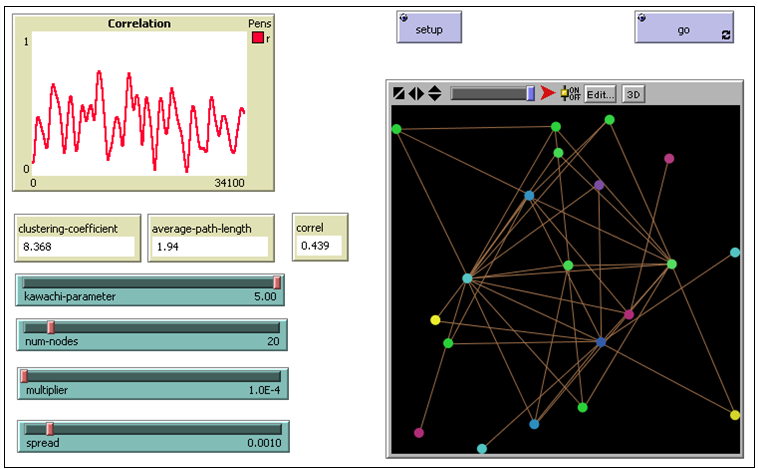
Figure 1: NetLogo simulation of the Kuramoto model for a scale-free network of 20 nodes. The coupling is set to $\sigma=10^{-4}$. The colours of the nodes in the network diagram visually represent the phase angles of the oscillators and give a sense of how many oscillators are locked (the green nodes in this snapshot) versus how many are drifting (other colours). The order parameter “correlation” shows incoherent behaviour consistent with the poorly coupled network failing to synchronise.

We next show two cases at coupling of $\sigma=2\times 10^{-4}$ at which quite different periodic behaviours in the order paramater can be seen. In the first instance, Fig.2, there is evidently a single oscillating mode. This behaviour has been reproduced a number of times though each case shows slightly different profiles according to the (small) number of nodes participating in such modes. However, other instances, for example shown in Fig.3, exhibit two superposed periodic modes. Again, a number of variations on this are observed for different random initial conditions and intrinsic frequencies.

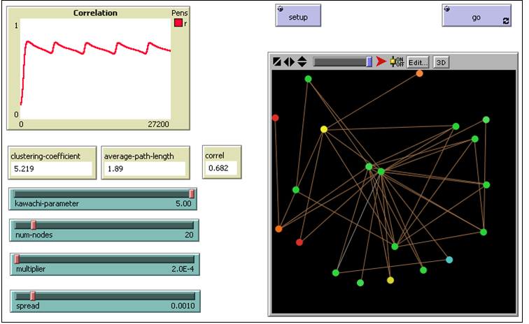
Figure 2: NetLogo simulation of the Kuramoto model for a scale-free network of 20 nodes. The coupling is set to $\sigma=2\times 10^{-4}$. The order parameter “correlation” shows periodic behaviour consistent with the limit cycle oscillation of a single mode. From the colours of the nodes we can see that many nodes are locked (green) while several (yellow and red) have not. This permits us to conclude that the limit cycle behaviour is not a consequence of a single oscillating node but of collections (albeit in small numbers) of nodes.

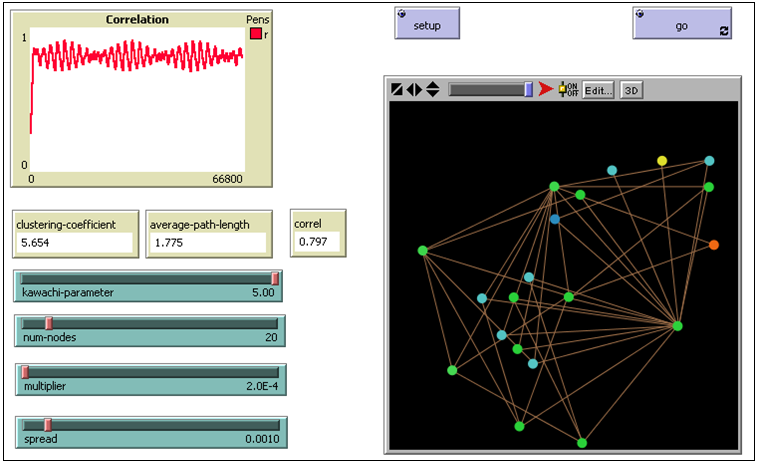
Figure 3: NetLogo simulation of the Kuramoto model for a scale-free network of 20 nodes. The coupling is set to $\sigma=2\times 10^{-4}$. The order parameter “correlation” shows periodic behaviour consistent with the limit cycle oscillation of two modes.

Finally, the coupling is increased to $\sigma=5\times 10^{-4}$ whence rapid synchronisation occurs as seen in Fig.4.

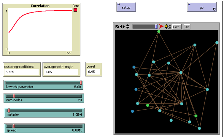
Figure 4: NetLogo simulation of the Kuramoto model for a scale-free network of 20 nodes. The coupling is set to $\sigma=5\times 10^{-4}$. The order parameter “correlation” shows rapid synchronisation.

These behaviours are consistent with those identified analytically for the one and two mode cases so that the periodicity is rather robust though the precise form it takes can vary according to randomness within the network and selection of intrinsic frequencies. Unfortunately, we are not able to extract the network properties directly from NetLogo in order to check the low-lying Laplacian spectral properties for these cases.

VI Discussion

We have considered second order approximations about the synchronised fixed point in the Kuramoto model on a general network. Motivated by insights from simulations that network sub-structures with smallest Laplacian eigenvalues approach synchronisation later in time, we have assumed higher modes to have reached steady state and analysed the dynamical equations for the remaining low-lying normal Laplacian modes. These equations resemble logistic and Lotka-Volterra equations and have yielded critical values for the coupling constant distinguishing behaviours such as convergence to the fixed point and limit cycles. In particular, this critical coupling is inversely proportional to the square of the algebraic connectivity. For larger numbers of low-lying modes participating in the dynamics more exotic dynamics can be exhibited, such as tori and chaos. In support of these results for one and two modes we have used NetLogo simulations to show evidence of periodic behaviour as the coupling is increased. This shows that for dynamical processes on networks there can be intermediate regimes of behaviour, between order (synchronisation) and chaos (incoherence), exhibiting rich structured behaviour, an example of Edge of Chaos phenomena.

At a broader level, these results show that for general networks there is no single critical coupling for the onset of synchronisation but many such coupling values indicating the regimes within which substructures can stabilise into states of partial synchronisation. We expect a similar hierarchy of couplings to be reflected in the nonperturbative regime, where the bulk of the normal modes have their dynamics “extinguished”. Our lack of analytical handle on the mechanism at play in this regime means we cannot yet compare with the case where this model all began, the complete graph: the high degeneracy of Laplacian eigenvalues here (infinite degeneracy for Kuramoto’s $N\rightarrow\infty$ case) means that the normal modes’ capacity to reach steady state lies entirely in this nonperturbative regime.

However, we can speculate to some degree on the role of Laplacian modes here. We notice that, whereas for regular graphs the Laplacian spectra are quite dispersed with multiple gaps between groups of (often degenerate) eigenvalues, for all known complex networks there occurs a clear accumulation of modes about some eigenvalue JamVanM : a “bulk” of modes is present in the spectrum. Erdös-Renyi random graphs generated by a low probability of creating a random link between any two nodes show this bulk at small eigenvalues while for large probability this bulk shifts up to higher values. Watts-Strogatz networks with small probability for rewiring a lattice graph have the bulk in a narrow curve around the mean nodal degree with smaller peaks reflecting the original spectrum for the lattice while for larger probability the main peak broadens. Finally, scale-free graphs have the main bulk occuring narrowly around eigenvalues of order unity with a few eigenvalues less than one. This bulk in the Laplacian spectrum is the common feature of any graph which, according to numerical studies, readily demonstrates synchronisation at finite values of the coupling.

A nonperturbative mechanism is therefore suggested: close-lying eigenmodes somehow mutually interfere with each other such as to cause them to de-excite to their steady states; when the majority of eigenvalues are closely spaced this de-excitation results in a large number of modes reaching steady state values. The threshold for this de-excitation is given by a critical coupling value. For the complete graph, the complete degeneracy of modes means this de-excitation across modes is nearly instantaneous. For other complex graphs this de-excitation takes some time to propagate, leaving some residual number of dynamical low-lying modes whose suppression has been the subject of this paper.

This insight suggests new approximations of the dynamical equations which may provide a handle on this nonperturbative mechanism. Our future work will seek to provide more substantial support to this hypothesis.

References

- (1) A. Kalloniatis, A new paradigm for modelling networked dynamical systems, 13th International Command and Control Research and Technology Symposium, Seattle USA, (2008)
- (2) N. Wiener, Nonlinear Problems in Random Theory, MIT Press, Cambridge (1958)
- (3) A.T. Winfree, J.Theoret.Biol, 16, 15 (1967).
- (4) Y. Kuramoto, Chemical Oscillations, Waves and Turbulence, Springer, Berlin (1984).
- (5) S.H. Strogatz, Physica D 143, 1 (2000).
- (6) J.A. Acebron, L.L. Bonilla, C.J. Perez Vicente, F. Ritort, R. Spigler, Rev.Mod.Phys.77, 137 (2005)
- (7) T. Ichinomiya, Phys.Rev.E 70, 026116 (2004)
- (8) J. Gomez-Gardenes, Y. Moreno, A. Arenas, Phys.Rev.E, 066106 (2007)
- (9) R. Albert, A.-L. Barabási, Rev.Mod.Phys. 74, 47 (2002)
- (10) D.J. Watts, S.H. Strogatz, Nature, 393, 440 (1998)
- (11) H. Hong, M.Y. Choi, B.J. Kim, Phys.Rev.E 65, 047104 (2002)
- (12) A. Arenas, A. Diaz-Guilera, C.J. Perez-Vicente, Phys. Rev. Lett. 96, 114102 (2006)
- (13) F.R.K. Chung, Spectral Graph Theory, CBMS, Regional Conference Series in Mathematics, No. 92, American Mathematical Society, Providence (1997)
- (14) B. Bollobás, Modern Graph Theory, Graduate Texts in Mathematics, Springer, USA, 1998
- (15) S.N. Dorogovstev, A.V. Goltsev, Rev.Mod.Phys. 80, 1275 (2008)
- (16) R.E. Mirollo, S.H. Strogatz, Physica D, 205, 249 (2005)
- (17) M. Fiedler, Czech. Math. J., 23, 298 (1973).
- (18) L.M. Pecora, T.L. Carroll, Phys.Rev.Lett. 80, 2109 (1998)
- (19) A.E. Motter, C. Zhou, J. Kurths, Phys.Rev.E 71, 016116 (2005); T. Nishikawa, A.E. Motter, Phys.Rev.E 73, 065106 (2006); B. Gong, L. Yang, K. Yang, Phys.Rev.E, 037101 (2005); Z.Li, G. Chen, IEEE Transactions on Circuits and Systems, 53, 28 (2006)
- (20) C.H.Q. Ding, X. He, H. Zha, Proceedings of the seventh ACM SIGKDD international conference on Knowledge discovery and data mining, p.275 (2001)
- (21) A. Jadbabaie, N. Motee, M. Barahona, Proceedings of the American Control Conference, Vol. 5., 4296 (2004).
- (22) D. Kaplan, L. Glass, Understanding Nonlinear Dynamics, Springer, NY (1995)
- (23) S. Smale, J.Math.Biol. 3,5 (1976)
- (24) J.C.Sprott, J.C. Wildenberg, Y. Azizi, Chaos, Solitons and Fractals, 26, 1035 (2005)
- (25) See http://ccl.northwestern.edu/netlogo.
- (26) A. Dekker, Journal of Artificial Societies and Social Simulation, 10 (4) 6; http://jasss.soc.surrey.ac.uk/10/4/6.html; the model can be downloaded from http://jasss.soc.surrey.ac.uk/10/4/6/resources/ NewKawachi.nlogo
- (27) Y. Kawachi, K. Murata, S. Yoshi, Y. Kakazu, Proc. 7th Asia-Pacific Conf. on Complex Systems, Australia, pp. 247-255, 2004
- (28) A. Jamakovic, P. van Mieghem, European Conference on Complex Systems, (2006)