Poissonian and non Poissonian Voronoi Diagrams with application to the aggregation of molecules

Abstract

The distributions that regulate the spatial domains of the Poissonian Voronoi Diagrams are discussed adopting the sum of gamma variate of argument two. The distributions that arise from the product and quotient of two gamma variates of argument two are also derived. Three examples of non Poissonian seeds for the Voronoi Diagrams are discussed. The developed algorithm allows the simulation of an aggregation of methanol and water.

url]http://www.ph.unito.it/$\tilde{~{}}$zaninett

1 Introduction

A great number of natural phenomena are described by Poissonian Voronoi diagrams , we cite some of them : lattices in quantum field theory [1] ; conductivity and percolation in granular composites [2, 3]; modeling growth of metal clusters on amorphous substrates [4]; the statistical mechanics of simple glass forming systems in $2D$ [5]; modeling of material interface evolution in grain growth of polycrystalline materials [6]. We now outline some applications in Chemistry. Detailed computer simulation results of several static and dynamical properties of water, obtained by using a realistic potential model were analyzed by evaluating the volume distributions of Voronoi polyhedron as well as angular and radial distributions of molecular clusters [7]. The local structure of three hydrogen bonded liquids comprising clusters of markedly different topology: water, methanol, and HF are investigated by analyzing the properties of the Voronoi polyhedron of the molecules in configurations obtained from Monte Carlo computer simulations [8]. The local lateral structure of dimyristoylphosphatidylcholine cholesterol mixed membranes of different compositions has been investigated on the basis of the Voronoi polygons [9]. Molecular dynamics simulation of a linear soft polymer has been performed and the free volume properties of the system have been analyzed in detail in terms of the Voronoi polyhedron of the monomers [10]. The molecular dynamics simulation of the aqueous solutions of urea of different concentrations are modeled by the method of Voronoi polyhedron [11].

From the point of view of the theory the only known analytical result for the Poissonian Voronoi diagrams , in the following $V-P$ after the two memories [12, 13] , is the size distribution in $1D$ . More precisely the theoretical distribution of segments in $1D$ is the gamma variate distribution of argument two , in the following $GV2$ [14]. The area in $2D$ and the volume in $3D$ were conjectured to follow the sum of two and three $GV2$ [14]. The possibility that the segments , area , and volume of $V-P$ can be modeled by a unique formula parametrized with $d$ which represents the considered dimension $d(d=1,2,3)$ has been recently analyzed [15]. Section 2 of this paper reviews the known formulas of the sum of $GV2$ and express them according to the chosen dimension. Section 3 explores the product and quotient of two $GV2$. Section 4 analyzes three examples of Voronoi Diagrams with correlated seeds or non Poissonian processes. Section 5 reports the simulation of an aggregation of methanol and water.

2 Sum of a Gamma variate

The starting point is the probability density function ( in the following PDF) in length , $s$ , of a segment in a random fragmentation

$$p(s)=\lambda\exp{(-\lambda s)}ds\quad,$$ (1)

where $\lambda$ is the hazard rate of the exponential distribution. Given the fact that the sum , $u$ , of two exponential distributions has a PDF

$$p(u)=\lambda^{2}u\exp{(-\lambda u)}du\quad.$$ (2)

The PDF of the $1D$ $V-P$ segments , $l$, ( the midpoint of the sum of two segments) can be found in the previous formula inserting $u=2l$

$$p(l)=2\lambda l\exp{(-2\lambda l)}d(2\lambda l)\quad.$$ (3)

When transformed in normalized units $x=\frac{l}{\lambda}$ the following PDF is obtained

$$p(x)=2x\exp{(-2x)}d(2x)\quad.$$ (4)

When this result is expressed as a gamma variate we obtain the PDF (formula (5) in [14])

$$H(x;c)=\frac{c}{\Gamma(c)}(cx)^{c-1}\exp(-cx)\quad,$$ (5)

where $0\leq x<\infty$ , $c~{}>0$ and $\Gamma(c)$ is the gamma function with argument c; in the case of $1D$ $V-P$ $c=2$. As an example Figure 1 reports the histogram of length of the normalized Voronoi segments in 1D.

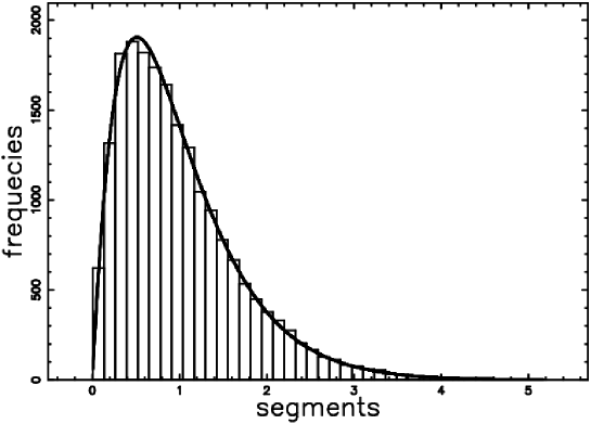
Figure 1: Histogram (step-diagram) of the $V-P$ normalized segment distribution in $1D$ with a superposition of the gamma–variate as represented by equation (8): the number of Poissonian seeds is 20000 , $d=1.02$ , $c=2.04$ , $NBIN=40$ and $\chi^{2}$=32.52 ,random seeds

The Kiang PDF has a mean of

$$\mu=1\quad,$$ (6)

and variance

$$\sigma^{2}=\frac{1}{c}\quad.$$ (7)

It was conjectured that the area in $2D$ and the volumes in $3D$ of the $V-P$ may be approximated as the sum of two and three $GV2$ . Due to the fact that the sum of n independent gamma variates with shape parameter $c_{i}$ is a gamma variate with shape parameter $c=\sum_{i}^{n}c_{i}$, the area and volumes are supposed to follow a gamma variate with argument 4 and 6  [16, 17]. This hypothesis was later named ”Kiang conjecture”, and equation (5) was used as a fitting function [18, 19, 20, 21], or as a hypothesis to accept or to reject using the standard procedures of the data analysis, see [22, 23]. The PDF (5) can be generalized by introducing the dimension of the considered space, $d(d=1,2,3)$ [23], [24]

$$H(x;d)=\frac{2d}{\Gamma(2d)}(2dx)^{2d-1}\exp(-2dx)\quad.$$ (8)

Two other PDFs give interesting results in the operation of fit of the $V-P$ area/volume. The first is the generalized gamma PDF with three parameters $(a,b,c)$ , [24, 15, 23] ,

$$f(x;b,c,d)=c\frac{b^{a/c}}{\Gamma(a/c)}x^{a-1}\exp{(-bx^{c})}\quad.$$ (9)

The generalized gamma PDF has the mean of

$$\mu=\frac{{b}^{-\frac{1}{c}}\Gamma\left(\frac{1+a}{c}\right)}{\Gamma\left({\frac{a}{c}}\right)}\quad,$$ (10)

and variance

$$\sigma^{2}=\frac{{b}^{-\frac{2}{c}}\left(+\Gamma\left({\frac{2+a}{c}}\right)\Gamma\left({\frac{a}{c}}\right)-\left(\Gamma\left({\frac{1+a}{c}}\right)\right)^{2}\right)}{\left(\Gamma\left({\frac{a}{c}}\right)\right)^{2}}\quad.$$ (11)

By the method of maximum likelihood the estimators , $\widehat{a}$, $\widehat{b}$ and $\widehat{c}$ are the solution to the simultaneous equations

$$\frac{n}{\widehat{c}}ln(\widehat{b})-n\frac{\Psi(\frac{\widehat{a}}{\widehat{c}})}{\widehat{c}}+\sum_{i=1}^{n}\ln(x_{i})=0$$

$$n\frac{\widehat{a}}{\widehat{c}}\frac{1}{\widehat{b}}-\sum_{i=1}^{n}\;x_{i}^{\widehat{c}}=0$$ (12)

$$\frac{n}{\widehat{c}}-n\frac{\widehat{a}}{{\widehat{c}}^{2}}ln(\widehat{b})+n\frac{\Psi(\frac{\widehat{a}}{\widehat{c}})\widehat{a}}{{\widehat{c}}^{2}}-{\widehat{b}}\sum_{i=1}^{n}\;x_{i}^{\widehat{c}}ln(x_{i})=0\quad,$$

where $\Psi(x)$ is the digamma function , $n$ the number of observations in a sample and $x_{i}$ is an observed value. The second one is a PDF of the type [15]

$$FN(x;d)=Const\times x^{\frac{3d-1}{2}}\exp{(-(3d+1)x/2)}\quad,$$ (13)

where

$$Const=\frac{\sqrt{2}\sqrt{3\,d+1}}{2\,{2}^{3/2\,d}\left(3\,d+1\right)^{-3/2\,d}\Gamma\left(3/2\,d+1/2\right)}\quad,$$ (14)

and $d(d=1,2,3)$ represents the dimension of the considered space. We will call the previously reported function the Ferenc-Neda PDF which has the mean of

$$\mu=1\quad,$$ (15)

and variance

$$\sigma^{2}=\frac{2}{3d+1}\quad.$$ (16)

Which distribution produces the best fit of the area of the irregular polygons and the volume of the irregular Polyhedron ? In order to answer this question we fitted the sample of the area and volume with the three distributions here considered . The 2D $V-P$ are reported in Figure 2 , Table 1 reports the $\chi^{2}$ results and Table 2 reports the parameters of generalized gamma deduced in two papers with the addition of our values.

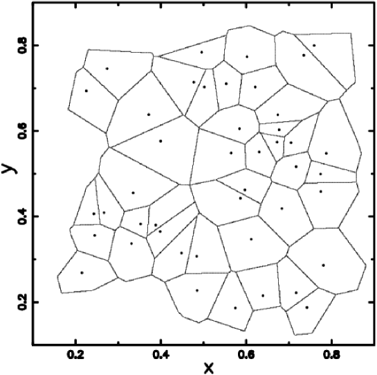
Figure 2: The $V-P$ in 2D. The selected region comprises 44 random seeds marked by a point.

Table 1: Values of $\chi^{2}$ for the cells normalized area-distribution function in 2D. Here we have 25087 Poissonian seeds and $40$ intervals in the histogram; $\nu$ denotes the degrees of freedom.

$$\begin{array}[]{lll}\hline\cr PDF{}&\nu{}&\chi^{2}\\ \vskip 3.0pt plus 1.0pt minus 1.0pt\cr\hline\cr\vskip 3.0pt plus 1.0pt minus 1.0pt\cr k(x;d)~{}(Eq.(\ref{kiangd}))~{},d=1.77&39&83.48\\ \vskip 3.0pt plus 1.0pt minus 1.0pt\cr f(x;d)~{}(Eq.(\ref{rumeni})){}&39&71.83\\ \vskip 3.0pt plus 1.0pt minus 1.0pt\cr G(x;a,b,c)~{}(Eq.(\ref{gammag}))&36&58.9\\ \vskip 3.0pt plus 1.0pt minus 1.0pt\cr h(x)~{}(Eq.(\ref{bessel}))&39&12636\\ \vskip 3.0pt plus 1.0pt minus 1.0pt\cr r(x)~{}(Eq.(\ref{ratio}))&39&19986\\ \hline\cr\hline\cr\end{array}$$

Table 2: Generalized gamma parameters $a$, $b$ and $c$ of the normalized area distribution in $2D$ in different papers with Poissonian seeds.

$$\begin{array}[]{lccc}\hline\cr reference&a&b&c\\ \vskip 3.0pt plus 1.0pt minus 1.0pt\cr\hline\cr\vskip 3.0pt plus 1.0pt minus 1.0pt\cr Ferenc-Neda~{}2007&2.29&3.01&1.08\\ Tanemura~{}1988~{}and~{}2003&3.31&3.04&1.078\\ this~{}paper&3.15&2.72&1.13\\ \\ \vskip 3.0pt plus 1.0pt minus 1.0pt\cr\hline\cr\hline\cr\end{array}$$

Figure 3 reports the various PDFs here adopted for the normalized area distribution in $2D$.

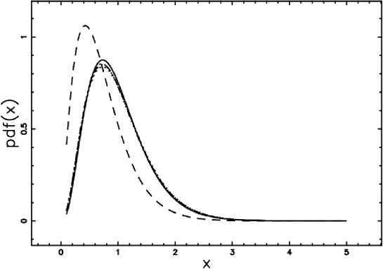
Figure 3: Poissonian seeds. Plot of the cells normalized area-distribution function in $2D$ when 5 PDFs are adopted : k(x ;d)  (Eq. (8)) ,d=1.87 (full line) , f(x;b,c,d) with data of Ferenc-Neda 2007 (dashed), f(x;b,c,d) with data of Tanemura 1988 and 2003 (dot-dash-dot-dash) , f(x;b,c,d) with our data (dotted) and f(x;d)  (Eq.(13)) ,d=2, (dash-dot-dot-dot) .

In $3D$ Figure 4 reports the histogram of the volume distribution as well as the Kiang’s PDF 8 when $d=3$ , Table 3 reports the $\chi^{2}$ results and Table 4 reports the parameters of generalized gamma in two papers with the addition of our values.

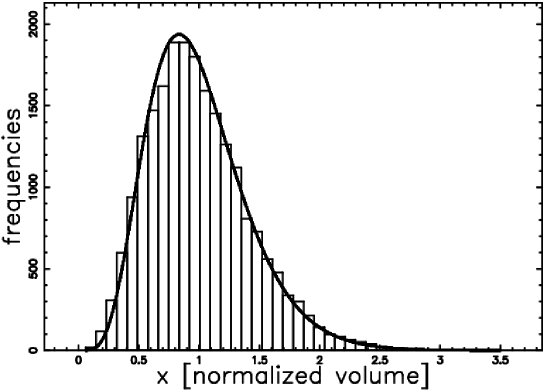
Figure 4: Histogram (step-diagram) of the $V-P$ normalized volume distribution in $3D$ with a superposition of the gamma–variate as represented by equation (8): the number of Poissonian seeds is 1392 , d=3, NBIN=40 and $\chi^{2}$=62.63 ,random seeds

Table 3: Values of $\chi^{2}$ for distribution of normalized volumes of $3D$ cells. Here 21378 Poissonian seeds were generated and $40$ interval were used in the histogram.

$$\begin{array}[]{llll}\hline\cr PDF{}&\nu{}&\chi^{2}\\ \vskip 3.0pt plus 1.0pt minus 1.0pt\cr\hline\cr\vskip 3.0pt plus 1.0pt minus 1.0pt\cr k(x;d)~{}(Eq.(\ref{kiangd}))~{},d=2.76&39&93.86\\ \vskip 3.0pt plus 1.0pt minus 1.0pt\cr f(x;d)~{}(Eq.(\ref{rumeni}),d=3){}&39&134.15\\ \vskip 3.0pt plus 1.0pt minus 1.0pt\cr G(x;a,b,c)~{}(Eq.(\ref{gammag}))&36&58.59\\ \hline\cr\hline\cr\end{array}$$

Table 4 reports the parameters of generalized gamma PDF deduced in two papers with the addition of our values.

Table 4: Generalized gamma parameters $a$ , $b$ and $c$ of the normalized volume distribution in $3D$ in different papers with Possonian seeds .

$$\begin{array}[]{lcccc}\hline\cr reference&a&b&c\\ \vskip 3.0pt plus 1.0pt minus 1.0pt\cr\hline\cr\vskip 3.0pt plus 1.0pt minus 1.0pt\cr Ferenc-Neda~{}2007&3.24&3.24&1.26\\ Tanemura~{}1988~{}and~{}2003&4.80&4.06&1.16\\ this~{}paper&4.68&3.87&1.18\\ \\ \vskip 3.0pt plus 1.0pt minus 1.0pt\cr\hline\cr\hline\cr\end{array}$$

Figure 5 reports the various PDFs here adopted for the normalized volume distribution in $3D$.

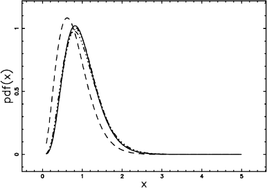
Figure 5: Poissonian seeds. Plot of the cells normalized volume-distribution function in $3D$ when 5 PDFs are adopted : k(x ;d)  (Eq. (8)) ,$d=2.79$ or $c=5.58$ (full line) , f(x;b,c,d) with data of Ferenc-Neda 2007 (dashed), f(x;b,c,d) with data of Tanemura 1988 and 2003 (dot-dash-dot-dash) , f(x;b,c,d) with our data (dotted) and f(x;d)  (Eq.(13)) ,d=3, (dash-dot-dot-dot) .

3 Product and Quotient of a Gamma variate

This Section explores the product XY and the quotient X/Y when X and Y are $GV2$.

3.1 Product

We recall that if $X$ is a random variable of the continuous type with PDF , $f(x)$, which is defined and positive on the interval $0\leq x<\infty$ and similarly if $Y$ is a random variable of the continuous type with PDF $g(y)$ which is defined and positive $0\leq y<\infty$ , the PDF of $V=XY$ is

$$h(v)=\int_{0}^{\infty}g(\frac{v}{x})f(x)\frac{1}{x}dx\quad.$$ (17)

Here the case of equal limits of integration will be explored , when this is not true difficulties arise [25, 26] . When $f(x)$ and $g(y)$ are $GV2$ the PDF is

$$h(v)=\int_{0}^{\infty}\frac{16\,{e^{-2\,x}}v{e^{-2\,{\frac{v}{x}}}}}{x}dx=32\,v{\it K_{0}}\left(4\,\sqrt{v}\right)\quad,$$ (18)

where $K_{\nu}(z)$ is the modified Bessel function of the second kind [27, 28] with $\nu$ representing the order, in our case 0. The previous integral can be solved with the substitution $x=\frac{y}{2}$ and using the integral representation in [29] , pag. 183

$$K_{\nu}(z)=\frac{1}{2}(\frac{1}{2}z)^{\nu}\int_{0}^{\infty}\exp\bigl{(}-\tau-\frac{z^{2}}{4\tau}\bigr{)}\frac{1}{\tau^{\nu+1}}d\tau\quad.$$ (19)

The mean of the new PDF, $h(v)$, as represented by formula (18) is

$$<v>=\int_{0}^{\infty}v\times 32\,v{\it K_{0}}\left(4\,\sqrt{v}\right)dv=1\quad.$$ (20)

The mode , $m$ , is at v =0.15067 and Table 1 reports the $\chi^{2}$ of the fit of the $V-P$ normalized area-distribution in $2D$.

3.2 The quotient

The PDF of $V=X/Y$ when X , represented by g(x) , and Y , represented by f(y) , are $GV2$ is

$$r(v)=\int_{0}^{\infty}|w|g({v}{x})f(x)dx=\frac{6\,v}{\left(1+v\right)^{2}\left(1+2\,v+{v}^{2}\right)}\quad.$$ (21)

The mean of the new PDF, $r(v)$, as represented by formula (21) is

$$<v>=\int_{0}^{\infty}v\times\frac{6\,v}{\left(1+v\right)^{2}\left(1+2\,v+{v}^{2}\right)}dv=2\quad.$$ (22)

The mode , $m$ , is at $v=\frac{1}{3}$ and Table 1 reports the $\chi^{2}$ of the fit of the Voronoi cell’s normalized area-distribution in 2D.

4 Non-Poissonian seeds

We now explore the case in which the seeds of the Voronoi Diagrams are distributed in a correlated way with respect to the center of the box. The correlated seeds are generated in polar coordinates , $\rho$ and $\theta$. The radius $\rho$ , the distance from the center of the box , is generated according to the PDF which is the product of two $GV2$ , see formula (18) once the scale parameter $b$ is introduced ,

$$h(v,b)=\frac{32\,v{\it K_{0}}\left(4\,\sqrt{\frac{v}{b}}\right)}{b^{2}}\quad.$$ (23)

Random numbers of the polar angle $\theta$ , in degrees, can be generated from those of the unit rectangular variate $R$ using the relationship

$$\theta\sim 360\times R\quad.$$ (24)

A typical example of Voronoi Diagrams generated by such seeds is reported in Figure 6 and Table (5) reports the $\chi^{2}$ of three different fits.

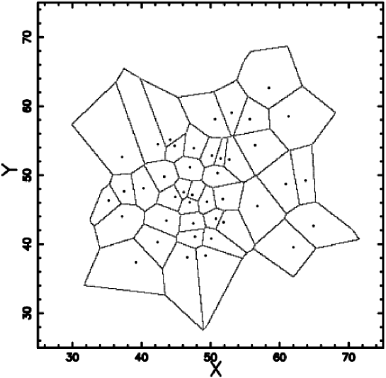
Figure 6: The Voronoi Diagram in 2D with Non-Poissonian seeds generated according to the product of two $GV2$ , see formula (23). The selected region comprises 42 random seeds marked by a point and $b=25$.

From a careful analysis of Table (5) it is possible to conclude that the product of two random variables, produces a better fit with respect to the Kiang function with fixed or variable $d$.

Table 5: Normalized area distribution in $2D$ of 166 correlated seeds generated according to formula (23). The $\chi^{2}$ of data fit when the number of classes is 40 for three PDF

$$\begin{array}[]{lll}\hline\cr PDF&name&\chi^{2}\\ \vskip 3.0pt plus 1.0pt minus 1.0pt\cr\hline\cr\vskip 3.0pt plus 1.0pt minus 1.0pt\cr H(x;d)&Kiang~{}PDF~{},formula~{}(\ref{kiangd})~{}when~{}d=2~{},&2142\\ \vskip 3.0pt plus 1.0pt minus 1.0pt\cr H(x;d)&Kiang~{}PDF~{},formula~{}(\ref{kiangd})~{}when~{}d=0.61~{},&43\\ \vskip 3.0pt plus 1.0pt minus 1.0pt\cr h(v)&product~{}two~{}gamma,formula~{}(\ref{bessel})&40\\ \vskip 3.0pt plus 1.0pt minus 1.0pt\cr\hline\cr\hline\cr\end{array}$$

Another example is represented by the ratio of two $GV2$ , formula (21) , that when the scale parameter $b$ is introduced has PDF

$$r(v,b)=\frac{6\,v{b}^{4}}{{b}^{2}\left(b+v\right)^{2}\left({b}^{2}+2\,vb+{v}^{2}\right)}\quad.$$ (25)

An example of Voronoi Diagrams generated by seeds that follow the quotient of two $GV2$ is reported in Figure 7 and Table 6 reports the $\chi^{2}$ of three different fits.

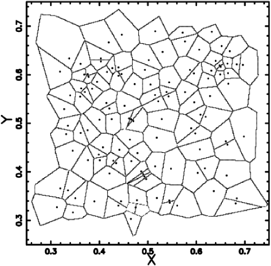
Figure 7: The Voronoi–diagram in $2D$ when the seeds are generated according to the quotient of two $GV2$ , see formula (25) . The selected region comprises 117 seeds and $b=25$.

Table 6: Normalized area distribution in $2D$ of 117 correlated seeds generated according to formula (25). The $\chi^{2}$ of data fit when the number of classes is 40 for three PDF

$$\begin{array}[]{lll}\hline\cr PDF&name&\chi^{2}\\ \vskip 3.0pt plus 1.0pt minus 1.0pt\cr\hline\cr\vskip 3.0pt plus 1.0pt minus 1.0pt\cr H(x;d)&Kiang~{}PDF~{},formula~{}(\ref{kiangd})~{}when~{}d=2~{},&5560\\ \vskip 3.0pt plus 1.0pt minus 1.0pt\cr H(x;d)&Kiang~{}PDF~{},formula~{}(\ref{kiangd})~{}when~{}d=1~{},&87\\ \vskip 3.0pt plus 1.0pt minus 1.0pt\cr r(v)&ratio~{}two~{}gamma,formula~{}(\ref{ratio})&79\\ \vskip 3.0pt plus 1.0pt minus 1.0pt\cr\hline\cr\hline\cr\end{array}$$

From a careful analysis of Table 6 it is possible to conclude that the quotient of two $GV2$ , also in this case produces a better fit with respect to the Kiang function with fixed or variable $d$.

A third example is represented by the Normal ( Gaussian ) distribution which has PDF

$$N(x;\sigma)=\frac{1}{\sigma(2\pi)^{1/2}}\exp({-{\frac{x^{2}}{2\sigma^{2}}}})\quad-\infty<x<\infty\quad.$$ (26)

When only positive values of $x$ are considered PDF (26) transforms in

$$HN(x;\sigma)=\frac{2}{\sigma(2\pi)^{1/2}}\exp({-{\frac{x^{2}}{2\sigma^{2}}}})\quad 0<x<\infty\quad.$$ (27)

We now consider the product of two normal random variables $X=N(0,1)$ and $Y=N(0,1)$. The PDF of $V=XY$ is [26]

$$hn(v)=\left\{\begin{array}[]{ll}K_{0}(v*signum(v))/\pi&-\infty<v<0\\ K_{0}(v*signum(v))/\pi&0<v<\infty~{}.\end{array}\right.$$ (28)

This PDF has a pole at $v=0$ and when the scale parameter $b$ is introduced and only positive values are considered it transforms in

$$hn(v;b)=2K_{0}(\frac{v}{b})/\pi\quad 0<v<\infty\quad.$$ (29)

An example of Voronoi Diagrams generated by seeds that follow the Half Normal (Gaussian) distribution (formula(27)) is reported in Figure 8 and Table 7 reports the $\chi^{2}$ of four different fits.

Table 7: Normalized area distribution in $2D$ of 145 correlated seeds generated according to formula (27), side=1, $\sigma=0.5$. The $\chi^{2}$ of data fit when the number of classes is 40 for three PDF

$$\begin{array}[]{lll}\hline\cr PDF&name&\chi^{2}\\ \vskip 3.0pt plus 1.0pt minus 1.0pt\cr\hline\cr\vskip 3.0pt plus 1.0pt minus 1.0pt\cr H(x;d)&Kiang~{}PDF~{},formula~{}(\ref{kiangd})~{}when~{}d=2~{},&2070\\ \vskip 3.0pt plus 1.0pt minus 1.0pt\cr H(x;d)&Kiang~{}PDF~{},formula~{}(\ref{kiangd})~{}when~{}d=0.88~{},&84\\ \vskip 3.0pt plus 1.0pt minus 1.0pt\cr HN(x;\sigma)&Half~{}Normal(Gaussian)~{}PDF,formula~{}(\ref{gaussianhalf})&168\\ \vskip 3.0pt plus 1.0pt minus 1.0pt\cr hn(v;b)&Product~{}two~{}Gaussian~{}PDF,formula~{}(\ref{productgauss})&78\\ \vskip 3.0pt plus 1.0pt minus 1.0pt\cr\hline\cr\hline\cr\end{array}$$

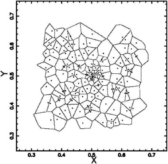
Figure 8: The Voronoi–diagram in $2D$ when the seeds are generated according to the Half Normal (Gaussian) distribution , see formula (27) . The selected region comprises 145 seeds ,$side=1$ and $\sigma=0.5$.

From a careful analysis of Table 7 it is possible to conclude that the product of two Gaussian PDFs produces a better fit with respect to the Half Normal (Gaussian) distribution and the Kiang function.

5 Aggregation of molecules

The analysis of the molecular dynamics through the Voronoi polyhedron in $3D$ or the Voronoi polygons in $2D$ is becoming a standard procedure. What is very interesting is the surface aggregation of a water-methanol mixture at 298 $K$, see [30]. The aggregation of the methanol and water molecules at the surface of their mixture is analyzed in the light of the Voronoi diagrams considering water and methanol molecules together , see Figure 11 in [30]. Figure 12 in [30] reports an instantaneous snapshot of the surface layer of a system containing 5 $\%$ methanol molecules (top view), as taken out from an equilibrium configuration. In order to simulate such an aggregate Figure 2 reports the $2D$ $V-P$ and Figure 9 the theoretical displacement of the molecules on such a network.

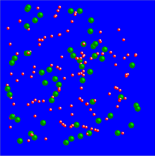
Figure 9: Superposed on the $V-P$ network of Figure 2 are present 131 molecules of water (red small balls) and 54 molecules of methanol (green great balls).

The same aggregate is simulated by non Poissonian seeds and Figure 6 reports the Voronoi Diagram while Figure 10 the theoretical displacement of the molecules on such correlated network.

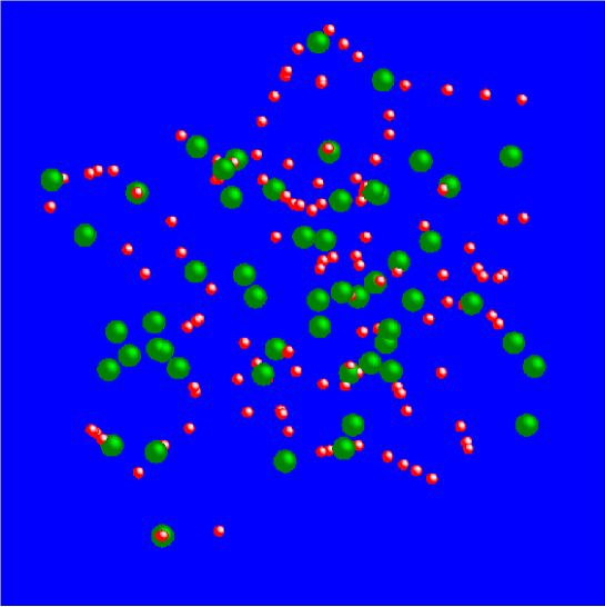
Figure 10: Superposed on the network of Figure 6 generated by non Poissonian seeds are present 131 molecules of water (red small balls) and 54 molecules of methanol (green great balls).

6 Conclusions

The size distribution of $V-P$ in $1D$ has an exact analytical result that is a $GV2$. Starting from this analytical result we derived the sum , the product and the quotient of two $GV2$. The area distribution of $V-P$ in $2D$ is well represented by the sum rather than the product of and quotient of two $GV2$ , see Table 1. A careful comparison between the Kiang function, formula (8) , and a new function suggested by Ferenc-Neda , see formula (13), has been done , see Table 1 and Table 3. In presence of non-Poissonian seeds that present a symmetry around the center the situation is inverted and the product of two $GV2$ , formula (18), or the ratio of two $GV2$ ,formula (21) , produce a better fit of the area distribution of Voronoi polygons in $2D$ with respect to the Kiang function, formula (8) , see Table 5 and Table 6. A third test made on Normal (Gaussian) correlated seeds is in agreement with the conjecture that the area of the $2D$ Voronoi diagrams follows the distribution of the seeds. The developed algorithm allows us to simulate some well studied aggregation such as the molecules of the water-methanol mixture. The question of whether if the area of the voids between molecules follows the $V-P$ area distribution as represented by the Kiang function , see equation (5) or the gamma of Ferenc-Neda , see equation (13) is open to future efforts.

References

- [1] J. M. Drouffe, C. Itzykson, Nuclear Physics B 235 (1984) 45.
- [2] G. R. Jerauld, J. C. Hatfield, L. E. Scriven, H. T. Davis, Journal of Physics C Solid State Physics 17 (1984) 1519.
- [3] G. R. Jerauld, L. E. Scriven, H. T. Davis, Journal of Physics C Solid State Physics 17 (1984) 3429.
- [4] S. B. Dicenzo, G. K. Wertheim, Phys. Rev. B39 (1989) 6792.
- [5] H. G. E. Hentschel, V. Ilyin, N. Makedonska, I. Procaccia, N. Schupper, Phys. Rev. E75 (5) (2007) 050404.
- [6] T.-Y. Lee, J. S. Chen, International Journal for Computational Methods in Engineering Science and Mechanics 7 (2006) 475.
- [7] G. Ruocco, M. Sampoli, A. Torcini, R. Vallauri, The Journal of Chemical Physics 99 (10) (1993) 8095.
- [8] P. Jedlovszky, Journal of Chemical Physics113 (2000) 9113.
- [9] P. Jedlovszky, N. N. Medvedev, M. Mezei, The Journal of Physical Chemistry B 108 (1) (2004) 465.
- [10] M. Sega, P. Jedlovszky, N. N. Medvedev, R. Vallauri, Journal of Chemical Physics121 (2004) 2422.
- [11] A. Idrissi, P. Damay, K. Yukichi, P. Jedlovszky, Journal of Chemical Physics129 (16) (2008) 164512.
- [12] G. Voronoi, Z. Reine Angew. Math 133 (1907) 97.
- [13] G. Voronoi, Z. Reine Angew. Math 134 (1908) 198.
- [14] T. Kiang, Zeitschrift fur Astrophysics 64 (1966) 433.
- [15] J.-S. Ferenc, Z. Néda, Physica A Statistical Mechanics and its Applications 385 (2007) 518.
- [16] W. Feller, An introduction to probability theory and its applications, Wiley, New York, 1971.
- [17] M. I. Tribelsky, Phys. Rev. Lett. 89 (7) (2002) 070201.
- [18] L. Zaninetti, Physics Letters A 165 (1992) 143.
- [19] S. Kumar, S. K. Kurtz, J. R. Banavar, S. M.G., Journal of Statistical Physics 67 (1992) 523.
- [20] L. Zaninetti, Chinese J. Astron. Astrophys.6 (2006) 387.
- [21] A. Korobov, Physical Review E 79 (2009) 031607.
- [22] M. Tanemura, J. Microscopy 151 (1988) 247.
- [23] M. Tanemura, Forma 18 (2003) 221.
- [24] A. L. Hinde , R. Miles, J. Stat. Comput. Simul. 10 (1980) 205.
- [25] M. Springer, The Algebra of Random Variables, Wiley, New York, 1979.
- [26] A. Glen, J. Leemis, L.M.and Drew, Computational Statistics & Data Analysis 44 (2004) 451.
- [27] M. Abramowitz, I. A. Stegun, Handbook of mathematical functions with formulas, graphs, and mathematical tables, Dover, New York, 1965.
- [28] W. H. Press, S. A. Teukolsky, W. T. Vetterling, B. P. Flannery, Numerical recipes in FORTRAN. The art of scientific computing, Cambridge University Press, Cambridge, 1992.
- [29] G. N. Watson, A Treatise on the Theory of Bessel Functions, Cambridge University Press, Cambridge, 1922.
- [30] L. B. Partay, P. Jedlovszky, A. Vincze, G. Horvai, The Journal of Physical Chemistry B 112 (17) (2008) 5428.