Jaynes-Cummings Models with trapped electrons on liquid Helium

Miao Zhang, H.Y. Jia and L.F. Wei111weilianfu@gmail.com Quantum Optoelectronics Laboratory and Institute of Modern Physics, Southwest Jiaotong University, Chengdu 610031, China
Abstract

Jaynes-Cummings model is a typical model in quantum optics and has been realized with various physical systems (e.g, cavity QED, trapped ions, and circuit QED etc..) of two-level atoms interacting with quantized bosonic fields. Here, we propose a new implementation of this model by using a single classical laser beam to drive an electron floating on liquid Helium. Two lowest levels of the vertical motion of the electron acts as a two-level β€œatom”, and the quantized vibration of the electron along one of the parallel directions, e.g., $x$-direction, serves the bosonic mode. These two degrees of freedom of the trapped electron can be coupled together by using a classical laser field. If the frequencies of the applied laser fields are properly set, the desirable Jaynes-Cummings models could be effectively realized.

PACS number(s): 42.50.Dv, 42.50.Ct, 73.20.-r.

Jaynes-Cummings model (JCM), describing the basic interaction of a two-level atom and a quantized electromagnetic field, is a cornerstone for the treatment of the interaction between light and matter in Quantum OpticsΒ JCM0 . This model can explain many quantum phenomena, such as the collapses and revivals of the atomic population inversions, squeezing of the quantized field, and the atom-cavity entanglement. Furthermore, recent experiments show that the JCMs can be implicated in quantum-state engineering and quantum information processing, e.g., generation of Fock statesΒ Fock and entangled statesΒ entangled , and the implementations of quantum logic gatesΒ gates , etc.. Originally, JCM is physically implemented with a cavity quantum electrodynamics (QED) system (see, e.g.,Β QED ). Certainly, there has been also interest to realize the Jaynes-Cummings Hamiltonian with other physical systems. A typical system is a cold ion trapped in a Paul trap and driven by classical laser beamsΒ trapped-ion ; Rev.Mod.trapped.ion ; JCMs1 . There, the interaction between two selected internal electronic levels and the external vibrational mode of the ion can be induced. Under the so-called Lamb-Dicke (LD) limit and the well-known rotating-wave approximation, the desirable JCM (or anti-JCM) can be realized by setting the applied laser frequencies with the suitable red (or blue) sideband excitations.

Recently, Platzman and Dykman have proposed that the electrons floating on liquid Helium could be utilized to implement quantum computationΒ Science ; PRB . In this proposal, electrons are trapped on the surface of liquid Helium and controlled by a series of external electric fields, which are generated by the micro-electrodes set below the liquid Helium. These electrons are effectively coupled together via their Coulomb interactions. By applying microwave radiation to these electrons from the micro-electrodes, their quantum states could be coherently controlled. Due to its scalability, easy manipulation, and relative long coherence time, this system has been paid much attention in recent years for quantum information processing (see, e.g.,Β Science ; PRB ; electron1 ; APL ; electron2 ).

In this paper, we further show, theoretically, that an electron floating on liquid Helium could also be utilized to realize the desirable JCMs. Inspired by the idea of implementing JCMs with trapped ions, we use a classical laser field to couple the vertical and parallel motional degrees of freedom of the electron on liquid Helium (similar to the laser-assisted coupling between the internal and external states of trapped ions).

We consider an electron floating on the surface of liquid Helium (e.g., ${}^{4}\text{He}$). The electron is weakly attracted by the dielectric image potential and strongly repulsed by the Pauli potential (i.e., Pauli exclusion principle), with about $1$eV potential barrier, to prevent it from penetrating into the liquid Helium. As a consequence, the electron’s motion normal to the liquid Helium surface can be approximately described by a one-dimensional ($1$D) hydrogen with the following potentialΒ Rev.Mod.Phys.

$$V(z)=\left\{\begin{array}[]{cc}-\frac{\Lambda e^{2}}{z}\,\,\,\,\,\,\,z>0,\\ \\ +\infty\,\,\,\,\,\,\,\,\,\,z\leq 0.\end{array}\right.$$ (1)

Where, $e$ is electron (with mass $m_{e}$) charge, $z$ is the distance above liquid Helium surface, and $\Lambda=(\varepsilon-1)/4(\varepsilon+1)$ with $\varepsilon=1.0568$ being dielectric constant of liquid ${}^{4}\text{He}$. The energy levels associated with this motion form a hydrogen-like spectrums $E_{n}=-\Lambda^{2}e^{4}m_{e}/2n^{2}\hbar^{2}\approx-0.00065/n^{2}$ eV, which has been experimentally observedΒ Grimes , and the corresponding wave functions can be written asΒ eigen-states

$$\psi_{n}(z)=2n^{-\frac{5}{2}}r_{B}^{-\frac{3}{2}}z\exp[-\frac{z}{nr_{B}}]L_{n-1}^{(1)}(\frac{2z}{nr_{B}}),$$ (2)

with the Bohr radius $r_{B}=\hbar^{2}/(m_{e}e^{2}\Lambda)\approx 76$Γ… and Laguerre polynomials

$$L_{n}^{(\alpha)}(x)=\frac{e^{x}x^{-\alpha}}{n!}\frac{d^{n}}{dx^{n}}[e^{-x}x^{n+\alpha}].$$ (3)
Refer to caption
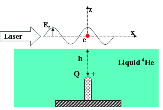
Figure 1: (Color online) A sketch of an electron confined by a micro-electode $Q$ submerged by the depth $h$ beneath the Helium surface and driven by a classical laser field propagating along the $x$-direction.

Beside the image potential (1), the electron is also trapped by another potential generated by the charge $Q$ on the micro-electrode, which is located at $h$ beneath the liquid Helium surfaceΒ PRB . The configuration of our model is shown in Fig.Β 1. For simplicity, on the Helium surface the electron is assumed to be effectively constrained to move only along the $x$-axes. Therefore, under the usual condition: $z,x<<h$, the total potential of the electron can be effectively approximated asΒ PRB

$$U(z,x)\approx-\frac{\Lambda e^{2}}{z}+eE_{\bot}z+\frac{1}{2}m_{e}\nu^{2}x^{2}$$ (4)

with $E_{\perp}\approx Q/h^{2}$ and $\nu\approx\sqrt{eQ/(m_{e}h^{3})}=\sqrt{eE_{\perp}/(m_{e}h)}$ . This indicates that the motions of the trapped electron can be regarded as a 1D Stark-shifted hydrogen along the $z$-direction, and a harmonic oscillation along the $x$-direction. Following Dykman et.al.Β PRB , only two lowest levels (i.e., the ground state $|g\rangle$ and first excited state $|e\rangle$) of the 1D Stark-shifted hydrogen are considered. As a consequence, the Hamiltonian describing these two uncoupled degrees of freedom of the electron reads

H^0=ℏ​ν​(a^†​a^+12)+ℏ​ω02​σ^z.subscript^𝐻0Planck-constant-over-2-pi𝜈superscript^π‘Žβ€ ^π‘Ž12Planck-constant-over-2-pisubscriptπœ”02subscript^πœŽπ‘§\hat{H}_{0}=\hbar\nu(\hat{a}^{\dagger}\hat{a}+\frac{1}{2})+\frac{\hbar\omega_{0}}{2}\hat{\sigma}_{z}. (5)

Here, a^†superscript^π‘Žβ€ \hat{a}^{\dagger} and $\hat{a}$ are the bosonic creation and annihilation operators of the vibrational quanta (with frequency $\nu$) of the electron’s oscillation along the $x$-direction. $\hat{\sigma}_{z}=|e\rangle\langle e|-|g\rangle\langle g|$ is the Pauli operator. The transition frequency $\omega_{0}$ is defined by $\omega_{0}=(E_{e}-E_{g})/\hbar$ with $E_{g}$ and $E_{e}$ being the corresponding energies of the lowest two levels, respectively.

In order to couple the above two uncoupled degrees of freedom of the electron, we now apply a classical laser beam $\mathscr{E}(x,t)$, propagating along the $x$-direction, to the trapped electron (see Fig.Β 1). This is similar to the approach in ion trap system for coupling the external and internal degrees of freedom of the ionΒ Rev.Mod.trapped.ion . Suppose that the applied laser beam (of wave-vector $k_{l}$, amplitude $E_{z}$, frequency $\omega_{l}$ and initial phase $\phi_{l}$) takes the form $\mathscr{E}(x,t)=E_{z}\hat{z}\cos(k_{l}x-\omega_{l}t+\phi_{l})$, i.e., its electric field is $z$-direction polarization, then the Hamiltonian of the driven electron floating on the Helium can be written as

$$\hat{H}=\hat{H}_{0}+ez\mathscr{E}(x,t).$$ (6)

Certainly, x=ℏ/2​me​ν​(a^+a^†)π‘₯Planck-constant-over-2-pi2subscriptπ‘šπ‘’πœˆ^π‘Žsuperscript^π‘Žβ€ x=\sqrt{\hbar/2m_{e}\nu}(\hat{a}+\hat{a}^{\dagger}), and thus the above Hamiltonian can be further written as

H^=H^0+ℏ​Ω~​σ^z​(ei​η​(a^+a^†)βˆ’i​ωl​t+i​ϕl+eβˆ’i​η​(a^+a^†)+i​ωl​tβˆ’i​ϕl)+ℏ​Ω​(Οƒ^βˆ’+Οƒ^+)​(ei​η​(a^+a^†)βˆ’i​ωl​t+i​ϕl+eβˆ’i​η​(a^+a^†)+i​ωl​tβˆ’i​ϕl),^𝐻subscript^𝐻0Planck-constant-over-2-pi~Ξ©subscript^πœŽπ‘§superscriptπ‘’π‘–πœ‚^π‘Žsuperscript^π‘Žβ€ π‘–subscriptπœ”π‘™π‘‘π‘–subscriptitalic-ϕ𝑙superscriptπ‘’π‘–πœ‚^π‘Žsuperscript^π‘Žβ€ π‘–subscriptπœ”π‘™π‘‘π‘–subscriptitalic-ϕ𝑙Planck-constant-over-2-piΞ©subscript^𝜎subscript^𝜎superscriptπ‘’π‘–πœ‚^π‘Žsuperscript^π‘Žβ€ π‘–subscriptπœ”π‘™π‘‘π‘–subscriptitalic-ϕ𝑙superscriptπ‘’π‘–πœ‚^π‘Žsuperscript^π‘Žβ€ π‘–subscriptπœ”π‘™π‘‘π‘–subscriptitalic-ϕ𝑙\begin{array}[]{l}\hat{H}=\hat{H}_{0}+\hbar\widetilde{\Omega}\hat{\sigma}_{z}(e^{i\eta(\hat{a}+\hat{a}^{\dagger})-i\omega_{l}t+i\phi_{l}}+e^{-i\eta(\hat{a}+\hat{a}^{\dagger})+i\omega_{l}t-i\phi_{l}})\\ \,\,\,\,\,\,\,\,\,\,\,\,\,+\hbar\Omega(\hat{\sigma}_{-}+\hat{\sigma}_{+})(e^{i\eta(\hat{a}+\hat{a}^{\dagger})-i\omega_{l}t+i\phi_{l}}+e^{-i\eta(\hat{a}+\hat{a}^{\dagger})+i\omega_{l}t-i\phi_{l}}),\end{array} (7)

with $\Omega=\langle g|z|e\rangle eE_{z}/(2\hbar)$ being the so-called carrier Rabi frequency describing the strength of coupling between the applied laser field and the electron, and Ξ©~=(⟨e|z|eβŸ©βˆ’βŸ¨g|z|g⟩)​e​Ez/(4​ℏ)β‰ 0~Ξ©quantum-operator-product𝑒𝑧𝑒quantum-operator-product𝑔𝑧𝑔𝑒subscript𝐸𝑧4Planck-constant-over-2-pi0\widetilde{\Omega}=(\langle e|z|e\rangle-\langle g|z|g\rangle)eE_{z}/(4\hbar)\neq 0 due to the broken parities of the quantum states of the above 1D hydrogen. Also, $\eta=k_{l}\sqrt{\hbar/2m_{e}\nu}$ is the so-called LD parameter, which describes the strength of coupling between the motions of $z$- and $x$-directions of the trapped electron. Finally, $\hat{\sigma}_{-}=|g\rangle\langle e|$ and $\hat{\sigma}_{+}=|e\rangle\langle g|$ are the usual raising and lowering operators, respectively. In the interaction picture defined by $\hat{U}(t)=\exp[(-i/\hbar)\hat{H}_{0}t]$, the Hamiltonian (7) reduces to

H^I=ℏ​Ω~​ei​ϕl​σ^z​eβˆ’i​ωl​t​ei​η​(a^​eβˆ’i​ν​t+a^†​ei​ν​t)+ℏ​Ω~​eβˆ’i​ϕl​σ^z​ei​ωl​t​eβˆ’i​η​(a^​eβˆ’i​ν​t+a^†​ei​ν​t)+ℏ​Ω​ei​ϕl​σ^βˆ’β€‹eβˆ’i​t​(Ο‰0+Ο‰l)​ei​η​(a^​eβˆ’i​ν​t+a^†​ei​ν​t)+ℏ​Ω​eβˆ’i​ϕl​σ^βˆ’β€‹eβˆ’i​t​(Ο‰0βˆ’Ο‰l)​eβˆ’i​η​(a^​eβˆ’i​ν​t+a^†​ei​ν​t)+ℏ​Ω​ei​ϕl​σ^+​ei​t​(Ο‰0βˆ’Ο‰l)​ei​η​(a^​eβˆ’i​ν​t+a^†​ei​ν​t)+ℏ​Ω​eβˆ’i​ϕl​σ^+​ei​t​(Ο‰0+Ο‰l)​eβˆ’i​η​(a^​eβˆ’i​ν​t+a^†​ei​ν​t).subscript^𝐻IPlanck-constant-over-2-pi~Ξ©superscript𝑒𝑖subscriptitalic-ϕ𝑙subscript^πœŽπ‘§superscript𝑒𝑖subscriptπœ”π‘™π‘‘superscriptπ‘’π‘–πœ‚^π‘Žsuperscriptπ‘’π‘–πœˆπ‘‘superscript^π‘Žβ€ superscriptπ‘’π‘–πœˆπ‘‘Planck-constant-over-2-pi~Ξ©superscript𝑒𝑖subscriptitalic-ϕ𝑙subscript^πœŽπ‘§superscript𝑒𝑖subscriptπœ”π‘™π‘‘superscriptπ‘’π‘–πœ‚^π‘Žsuperscriptπ‘’π‘–πœˆπ‘‘superscript^π‘Žβ€ superscriptπ‘’π‘–πœˆπ‘‘Planck-constant-over-2-piΞ©superscript𝑒𝑖subscriptitalic-ϕ𝑙subscript^𝜎superscript𝑒𝑖𝑑subscriptπœ”0subscriptπœ”π‘™superscriptπ‘’π‘–πœ‚^π‘Žsuperscriptπ‘’π‘–πœˆπ‘‘superscript^π‘Žβ€ superscriptπ‘’π‘–πœˆπ‘‘Planck-constant-over-2-piΞ©superscript𝑒𝑖subscriptitalic-ϕ𝑙subscript^𝜎superscript𝑒𝑖𝑑subscriptπœ”0subscriptπœ”π‘™superscriptπ‘’π‘–πœ‚^π‘Žsuperscriptπ‘’π‘–πœˆπ‘‘superscript^π‘Žβ€ superscriptπ‘’π‘–πœˆπ‘‘Planck-constant-over-2-piΞ©superscript𝑒𝑖subscriptitalic-ϕ𝑙subscript^𝜎superscript𝑒𝑖𝑑subscriptπœ”0subscriptπœ”π‘™superscriptπ‘’π‘–πœ‚^π‘Žsuperscriptπ‘’π‘–πœˆπ‘‘superscript^π‘Žβ€ superscriptπ‘’π‘–πœˆπ‘‘Planck-constant-over-2-piΞ©superscript𝑒𝑖subscriptitalic-ϕ𝑙subscript^𝜎superscript𝑒𝑖𝑑subscriptπœ”0subscriptπœ”π‘™superscriptπ‘’π‘–πœ‚^π‘Žsuperscriptπ‘’π‘–πœˆπ‘‘superscript^π‘Žβ€ superscriptπ‘’π‘–πœˆπ‘‘\begin{array}[]{l}\hat{H}_{\text{I}}=\hbar\widetilde{\Omega}e^{i\phi_{l}}\hat{\sigma}_{z}e^{-i\omega_{l}t}e^{i\eta(\hat{a}e^{-i\nu t}+\hat{a}^{\dagger}e^{i\nu t})}+\hbar\widetilde{\Omega}e^{-i\phi_{l}}\hat{\sigma}_{z}e^{i\omega_{l}t}e^{-i\eta(\hat{a}e^{-i\nu t}+\hat{a}^{\dagger}e^{i\nu t})}\\ \,\,\,\,\,\,\,\,\,\,\,\,\,\,+\hbar\Omega e^{i\phi_{l}}\hat{\sigma}_{-}e^{-it(\omega_{0}+\omega_{l})}e^{i\eta(\hat{a}e^{-i\nu t}+\hat{a}^{\dagger}e^{i\nu t})}+\hbar\Omega e^{-i\phi_{l}}\hat{\sigma}_{-}e^{-it(\omega_{0}-\omega_{l})}e^{-i\eta(\hat{a}e^{-i\nu t}+\hat{a}^{\dagger}e^{i\nu t})}\\ \,\,\,\,\,\,\,\,\,\,\,\,\,\,+\hbar\Omega e^{i\phi_{l}}\hat{\sigma}_{+}e^{it(\omega_{0}-\omega_{l})}e^{i\eta(\hat{a}e^{-i\nu t}+\hat{a}^{\dagger}e^{i\nu t})}+\hbar\Omega e^{-i\phi_{l}}\hat{\sigma}_{+}e^{it(\omega_{0}+\omega_{l})}e^{-i\eta(\hat{a}e^{-i\nu t}+\hat{a}^{\dagger}e^{i\nu t})}.\end{array} (8)

Now, we assume that the frequencies of the applied laser fields are sequentially set as $\omega_{l}=\omega_{0}+K\nu$ with $K=0,\pm 1$ corresponding to the usual resonance ($K=0$), the first blue-($K=1$) and red-($K=-1$) sidebands excitationsΒ Weistates , respectively. The LD parameters introduced above become $\eta=(\omega_{0}+K\nu)\sqrt{\hbar/(2m_{e}\nu)}/c$ (where $c$ is the velocity of light) and are sensitive to the frequencies $\omega_{0}$ and $\nu$, which are further relative to the applied trap field $E_{\perp}$ and the depth $h$ of the micro-electrode set beneath the liquid Helium surface. Under the well-known LD approximationΒ Rev.Mod.trapped.ion with $\eta\ll 1$, we have exp⁑[Β±i​η​(a^​eβˆ’i​ν​t+a^†​ei​ν​t)]β‰ˆ1Β±i​η​(a^​eβˆ’i​ν​t+a^†​ei​ν​t)plus-or-minusπ‘–πœ‚^π‘Žsuperscriptπ‘’π‘–πœˆπ‘‘superscript^π‘Žβ€ superscriptπ‘’π‘–πœˆπ‘‘plus-or-minus1π‘–πœ‚^π‘Žsuperscriptπ‘’π‘–πœˆπ‘‘superscript^π‘Žβ€ superscriptπ‘’π‘–πœˆπ‘‘\exp[\pm i\eta(\hat{a}e^{-i\nu t}+\hat{a}^{\dagger}e^{i\nu t})]\approx 1\pm i\eta(\hat{a}e^{-i\nu t}+\hat{a}^{\dagger}e^{i\nu t}) and simplify the above Hamiltonian to

H^IL​(t)=ℏ​Ω~​ei​ϕl​σ^z​[eβˆ’i​(Ο‰0+K​ν)​t+i​η​(a^​eβˆ’i​(Ο‰0+K​ν+Ξ½)​t+a^†​eβˆ’i​(Ο‰0+Kβ€‹Ξ½βˆ’Ξ½)​t)]+ℏ​Ω~​eβˆ’i​ϕl​σ^z​[ei​(Ο‰0+K​ν)​tβˆ’i​η​(a^​ei​(Ο‰0+Kβ€‹Ξ½βˆ’Ξ½)​t+a^†​ei​(Ο‰0+K​ν+Ξ½)​t)]+ℏ​Ω​ei​ϕl​σ^βˆ’β€‹[eβˆ’i​(2​ω0+K​ν)​t+i​η​(a^​eβˆ’i​(2​ω0+K​ν+Ξ½)​t+a^†​eβˆ’i​(2​ω0+Kβ€‹Ξ½βˆ’Ξ½)​t)]+ℏ​Ω​eβˆ’i​ϕl​σ^βˆ’β€‹[ei​K​ν​tβˆ’i​η​(a^​ei​(Kβˆ’1)​ν​t+a^†​ei​(K+1)​ν​t)]+ℏ​Ω​ei​ϕl​σ^+​[eβˆ’i​K​ν​t+i​η​(a^​eβˆ’i​(K+1)​ν​t+a^†​ei​(1βˆ’K)​ν​t)]+ℏ​Ω​eβˆ’i​ϕl​σ^+​[ei​(2​ω0+K​ν)​tβˆ’i​η​(a^​ei​(2​ω0+Kβ€‹Ξ½βˆ’Ξ½)​t+a^†​ei​(2​ω0+K​ν+Ξ½)​t)].superscriptsubscript^𝐻IL𝑑Planck-constant-over-2-pi~Ξ©superscript𝑒𝑖subscriptitalic-ϕ𝑙subscript^πœŽπ‘§delimited-[]superscript𝑒𝑖subscriptπœ”0πΎπœˆπ‘‘π‘–πœ‚^π‘Žsuperscript𝑒𝑖subscriptπœ”0πΎπœˆπœˆπ‘‘superscript^π‘Žβ€ superscript𝑒𝑖subscriptπœ”0πΎπœˆπœˆπ‘‘Planck-constant-over-2-pi~Ξ©superscript𝑒𝑖subscriptitalic-ϕ𝑙subscript^πœŽπ‘§delimited-[]superscript𝑒𝑖subscriptπœ”0πΎπœˆπ‘‘π‘–πœ‚^π‘Žsuperscript𝑒𝑖subscriptπœ”0πΎπœˆπœˆπ‘‘superscript^π‘Žβ€ superscript𝑒𝑖subscriptπœ”0πΎπœˆπœˆπ‘‘Planck-constant-over-2-piΞ©superscript𝑒𝑖subscriptitalic-ϕ𝑙subscript^𝜎delimited-[]superscript𝑒𝑖2subscriptπœ”0πΎπœˆπ‘‘π‘–πœ‚^π‘Žsuperscript𝑒𝑖2subscriptπœ”0πΎπœˆπœˆπ‘‘superscript^π‘Žβ€ superscript𝑒𝑖2subscriptπœ”0πΎπœˆπœˆπ‘‘Planck-constant-over-2-piΞ©superscript𝑒𝑖subscriptitalic-ϕ𝑙subscript^𝜎delimited-[]superscriptπ‘’π‘–πΎπœˆπ‘‘π‘–πœ‚^π‘Žsuperscript𝑒𝑖𝐾1πœˆπ‘‘superscript^π‘Žβ€ superscript𝑒𝑖𝐾1πœˆπ‘‘Planck-constant-over-2-piΞ©superscript𝑒𝑖subscriptitalic-ϕ𝑙subscript^𝜎delimited-[]superscriptπ‘’π‘–πΎπœˆπ‘‘π‘–πœ‚^π‘Žsuperscript𝑒𝑖𝐾1πœˆπ‘‘superscript^π‘Žβ€ superscript𝑒𝑖1πΎπœˆπ‘‘Planck-constant-over-2-piΞ©superscript𝑒𝑖subscriptitalic-ϕ𝑙subscript^𝜎delimited-[]superscript𝑒𝑖2subscriptπœ”0πΎπœˆπ‘‘π‘–πœ‚^π‘Žsuperscript𝑒𝑖2subscriptπœ”0πΎπœˆπœˆπ‘‘superscript^π‘Žβ€ superscript𝑒𝑖2subscriptπœ”0πΎπœˆπœˆπ‘‘\begin{array}[]{l}\hat{H}_{\text{I}}^{\text{L}}(t)=\hbar\widetilde{\Omega}e^{i\phi_{l}}\hat{\sigma}_{z}[e^{-i(\omega_{0}+K\nu)t}+i\eta(\hat{a}e^{-i(\omega_{0}+K\nu+\nu)t}+\hat{a}^{\dagger}e^{-i(\omega_{0}+K\nu-\nu)t})]\\ \,\,\,\,\,\,\,\,\,\,\,\,\,\,\,\,\,\,\,\,\,\par+\hbar\widetilde{\Omega}e^{-i\phi_{l}}\hat{\sigma}_{z}[e^{i(\omega_{0}+K\nu)t}-i\eta(\hat{a}e^{i(\omega_{0}+K\nu-\nu)t}+\hat{a}^{\dagger}e^{i(\omega_{0}+K\nu+\nu)t})]\\ \,\,\,\,\,\,\,\,\,\,\,\,\,\,\,\,\,\,\,\,\,\par+\hbar\Omega e^{i\phi_{l}}\hat{\sigma}_{-}[e^{-i(2\omega_{0}+K\nu)t}+i\eta(\hat{a}e^{-i(2\omega_{0}+K\nu+\nu)t}+\hat{a}^{\dagger}e^{-i(2\omega_{0}+K\nu-\nu)t})]\\ \,\,\,\,\,\,\,\,\,\,\,\,\,\,\,\,\,\,\,\,\,\par+\hbar\Omega e^{-i\phi_{l}}\hat{\sigma}_{-}[e^{iK\nu t}-i\eta(\hat{a}e^{i(K-1)\nu t}+\hat{a}^{\dagger}e^{i(K+1)\nu t})]\\ \,\,\,\,\,\,\,\,\,\,\,\,\,\,\,\,\,\,\,\,\,\par+\hbar\Omega e^{i\phi_{l}}\hat{\sigma}_{+}[e^{-iK\nu t}+i\eta(\hat{a}e^{-i(K+1)\nu t}+\hat{a}^{\dagger}e^{i(1-K)\nu t})]\\ \,\,\,\,\,\,\,\,\,\,\,\,\,\,\,\,\,\,\,\,\,\par+\hbar\Omega e^{-i\phi_{l}}\hat{\sigma}_{+}[e^{i(2\omega_{0}+K\nu)t}-i\eta(\hat{a}e^{i(2\omega_{0}+K\nu-\nu)t}+\hat{a}^{\dagger}e^{i(2\omega_{0}+K\nu+\nu)t})].\par\end{array} (9)

Neglecting the above rapidly-oscillating terms (i.e., under the usual rotating-wave approximation)Β RWA , this Hamiltonian can be further simplified to

$$\hat{H}_{\text{eff}}^{0}=\hbar\Omega e^{i\phi_{l}}\hat{\sigma}_{+}+H.c\,\,\,\,\,\,\,\,\,\,\,\,\,\,\,\,\,\,\,\text{for}\,\,\,K=0,$$ (10)
$$\hat{H}_{\text{eff}}^{\text{r}}=i\eta\hbar\Omega e^{i\phi_{l}}\hat{\sigma}_{+}\hat{a}+H.c\,\,\,\,\,\,\,\,\,\,\text{for}\,\,\,K=-1,$$ (11)
H^effb=i​η​ℏ​Ω​ei​ϕl​σ^+​a^†+H.cfor​K=1.formulae-sequencesuperscriptsubscript^𝐻effbπ‘–πœ‚Planck-constant-over-2-piΞ©superscript𝑒𝑖subscriptitalic-ϕ𝑙subscript^𝜎superscript^π‘Žβ€ π»π‘for𝐾1\hat{H}_{\text{eff}}^{\text{b}}=i\eta\hbar\Omega e^{i\phi_{l}}\hat{\sigma}_{+}\hat{a}^{\dagger}+H.c\,\,\,\,\,\,\,\,\,\,\text{for}\,\,\,K=1. (12)

Obviously, Hamiltonians $\hat{H}_{\text{eff}}^{\text{r}}$ and $\hat{H}_{\text{eff}}^{\text{b}}$ are nothing but just those of the usual JCM and anti-JCM, respectively. All the dynamical evolutions corresponding to the above effective Hamiltonians (10-12) are exactly solvable. For example, if the $x$-direction’s harmonic oscillator is prepared initially at the Fock state $|m\rangle$ ($m$ is its occupation number), then we have

i) For $K\leq 0$

$\displaystyle\left\{\begin{array}[]{l}|m\rangle|g\rangle\longrightarrow|m\rangle|g\rangle,\,\,m<k,\\ |m\rangle|g\rangle\longrightarrow\cos(\Omega_{m-k,k}t)|m\rangle|g\rangle+i^{k-1}e^{i\theta_{L}}\sin(\Omega_{m-k,k}t)|m-k\rangle|e\rangle;\,\,m\geq k,\\ |m\rangle|e\rangle\longrightarrow\cos(\Omega_{m,k}t)|m\rangle|e\rangle-(-i)^{k-1}e^{-i\theta_{L}}\sin(\Omega_{m,k}t)|m+k\rangle|g\rangle\end{array}\right.$ (16)

ii) For $K\geq 0$

$\displaystyle\left\{\begin{array}[]{l}|m\rangle|g\rangle\longrightarrow\cos(\Omega_{m,k}t)|m\rangle|g\rangle+i^{k-1}e^{i\theta_{L}}\sin(\Omega_{m,k}t)|m+k\rangle|e\rangle,\\ |m\rangle|e\rangle\longrightarrow|m\rangle|e\rangle,\,m<k,\\ |m\rangle|e\rangle\longrightarrow\cos(\Omega_{m-k,k}t)|m\rangle|e\rangle-(-i)^{k-1}e^{-i\theta_{L}}\sin(\Omega_{m-k,k}t)|m-k\rangle|g\rangle,\,m\geq k,\end{array}\right.$ (20)

with $\Omega_{m,k}=\Omega\eta^{k}\sqrt{(m+k)!/m!}$ being the effective Rabi frequency, and $k=|K|$. In principle, arbitrary quantum state engineering, e.g., generations of nonclassical quantum states and implementations of quantum logic gates, etc.Β gates ; JCMs1 ; Rev.Mod.trapped.ion , could be realized by the above evolutions.

The experimental feasibility of the JCMs proposed here involves with two important factors: the value of the introduced LD parameter $\eta$ and the decoherence of the electron. In fact, decoherence is always a challenge in various quantum coherence systems. Platzman and DykmanΒ PRB showed that the main source of decoherence in the present system is the so-called ripplons, i.e, the thermally excited surface waves of liquid HeliumΒ PRB ; Science . The coherence time due to this fluctuation is estimatedΒ PRB ; Science to be $10^{-4}$Β s (for the typical frequencies: a few tens of GHz), but could be increased by enhancing the frequency of the electron vibrating in-plane.

For the typical parameters EβŸ‚β‰ˆ104subscript𝐸perpendicular-tosuperscript104E_{\perp}\approx 10^{4}V/m and hβ‰ˆ5Γ—10βˆ’7β„Ž5superscript107h\approx 5\times 10^{-7}mΒ PRB , the transition frequency of the z𝑧z-direction’s 1D hydrogen and the vibrational frequency of the xπ‘₯x-direction’s oscillation are estimated as Ο‰0β‰ˆ1133subscriptπœ”01133\omega_{0}\approx 1133Β GHz and Ξ½β‰ˆ59𝜈59\nu\approx 59Β GHz, respectively. Consequently, the LD parameter in the above JCM is Ξ·β‰ˆ1.2Γ—10βˆ’4β‰ͺ1πœ‚1.2superscript104much-less-than1\eta\approx 1.2\times 10^{-4}\ll 1. Thus, the usual LD approximation is valid. Note that the LD parameter in present system is significantly smaller than that (there η∼0.2similar-toπœ‚0.2\eta\sim 0.2) in the experimental ion trap systemΒ JCMs1 ; Rev.Mod.trapped.ion . This is because the β€œatomic” frequency Ο‰0subscriptπœ”0\omega_{0} of the trapped ion (∼106similar-toabsentsuperscript106\sim 10^{6} GHz) is significantly larger than that in the present system (∼1similar-toabsent1\sim 1THz), and the vibrational frequency ν𝜈\nu (∼10βˆ’4similar-toabsentsuperscript104\sim 10^{-4} GHz) is significantly however smaller than that in the present system. Note that the LD parameters could, in principle, been enlarged by decreasing the value of ν𝜈\nu (by properly adjusting EβŸ‚subscript𝐸perpendicular-toE_{\perp} and hβ„Žh, e.g., Ξ·β‰ˆ0.16πœ‚0.16\eta\approx 0.16, Ο‰0β‰ˆ739subscriptπœ”0739\omega_{0}\approx 739Β GHz, Ξ½β‰ˆ13.3𝜈13.3\nu\approx 13.3Β KHz for EβŸ‚=10βˆ’5subscript𝐸perpendicular-tosuperscript105E_{\perp}=10^{-5}Β V/m and h=10βˆ’2β„Žsuperscript102h=10^{-2}Β m). However, ripplons-induced decoherence affects stronger for the smaller frequency of the vibrations in the plane (correspond to a large in-plane localization length).

Fortunately, although the LD parameters in present system are relatively small, the JCMs presented above still work within the typical coherence time ($\sim 10^{-4}$s). Our numerical estimations show that the duration of a $\pi$-pulse is $t=\pi/\Omega_{m,k}<10^{-4}$s. For example, if the amplitude of the applied laser field is set as the typical value: $E_{z}=10^{2}$V/mΒ PRB , and the LD parameter $\eta=1.2\times 10^{-4}$, we have $\pi/\Omega_{m,0}\approx 9.1\times 10^{-9}$s and $\pi/\Omega_{m,1}<7.6\times 10^{-5}$s. Note that the occupation number $m$ does not affect the values of $t=\pi/\Omega_{m,0}$, while $t=\pi/\Omega_{m,1}$ decreases with the increase of $m$ ($t\propto 1/\sqrt{m+1}$). Also, the above durations could be further shortened (such that the JCMs admit more $\pi$-pulse operations) by effectively increasing the amplitude $E_{z}$ of the applied laser field (i.e., increasing the carrier Rabi frequency $\Omega$). In principle, if the $E_{z}$ increases ten times, then the duration of a $\pi$-pulse shortens ten times. Indeed, for $E_{z}=10^{3}~{}V/m$ a $\pi$-pulse could be less than $7.6\times 10^{-6}$Β s.

The standard JCM requires that the bosonic field should be in a pure state. However, thermal states

$$\rho_{t}=\sum_{m=0}^{\infty}\frac{\langle m\rangle^{m}}{(1+\langle m\rangle)^{m+1}}|m\rangle\langle m|,\,\,\,\,\langle m\rangle=\frac{1}{e^{\hbar\nu/(k_{B}T)}-1},$$ (21)

are the natural states of the vibrational particles (e.g., trapped ionsΒ JCMs1 and the electrons in the present model), which are normally in thermal equilibrium with their surroundings.

Refer to caption
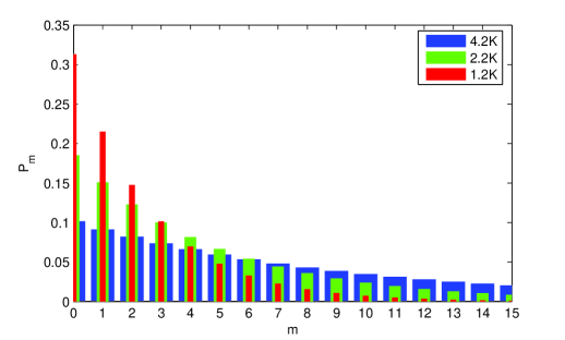
Figure 2: (Color online) Phonon distributions $P_{m}$ versus occupation number $m$ of (vibrational) frequency $\nu=59$GHz in the thermal states for the typical temperatures $T=4.2$K, $2.2$K, and $1.2$K.

Above, kBsubscriptπ‘˜π΅k_{B} and T𝑇T are the Boltzmann constant and the temperature of the surroundings, respectively. Fig.2 shows the phonon distribution of a thermal state for a vibration with frequency Ξ½=59𝜈59\nu=59 GHz (corresponding to 0.450.450.45K) at various typical temperatures: T=4.2𝑇4.2T=4.2K, 2.22.22.2K, and 1.21.21.2K. Obviously, if the temperature of the surrounding is further lower, the probabilities that the electron in the states with smaller occupations are much larger. Suppose that the liquid Helium is cooled to T=0.01𝑇0.01T=0.01KΒ PRB , which is much colder than 0.450.450.45K of the vibrational electronΒ PRB , then ρtβ‰ˆ|0βŸ©β€‹βŸ¨0|subscriptπœŒπ‘‘ket0bra0\rho_{t}\approx|0\rangle\langle 0| and thus the electronic vibration is well limited to the vacuum state.

In addition, the presented JCMs could be utilized to cool the vibrational electron. Indeed, if the out-plane state of the electron is initially in $|g\rangle$, a vibrational energy $\hbar\nu$ could be reduced by the following two steps: (i) apply a $\pi/2$-pulse with duration $t=\pi/2\Omega_{m-1,1}$ to drive a transition: $|m\rangle|g\rangle\rightarrow|m-1\rangle|e\rangle$; (ii) drive the transition $|e\rangle\rightarrow|g\rangle$ but forbid the transition $|g\rangle\rightarrow|e\rangle$ by using an auxiliary atomic level $|a\rangle$ and two resonant $\pi/2$-pulses to drive the transitions $|e\rangle\rightarrow|a\rangle\rightarrow|g\rangle$. For example, if the third level of the electron is selected to be the auxiliary level $|a\rangle$, we have $\omega_{ea}/\omega_{ge}\approx 0.18$ with $\omega_{ea}$ being the transition frequency between $|e\rangle$ and $|a\rangle$ and $\omega_{ge}$ between $|g\rangle$ and $|e\rangle$. After these two steps, cooling the vibrational electron by a $\hbar\nu$ is possible:

$$|m\rangle|g\rangle{\longrightarrow}|m-1\rangle|e\rangle{\longrightarrow}|m-1\rangle|a\rangle{\longrightarrow}|m-1\rangle|g\rangle.$$ (22)

These operations (their durations are typically less than $4\times 10^{-6}$Β s for $E_{z}=10^{3}$V/m) are repeated until the vibrational state $|m\rangle$ relaxes finally to the desirable ground state $|0\rangle$. As a consequence, an arbitrary mix state $\rho=\sum_{m}P_{m}|m\rangle\langle m|$ (with $P_{m}$ being the classical probability that the electron is in the vibrational state $|m\rangle$) could be cooled to the vibrational vacuum state $|0\rangle$. Note that the above method is similar to the so-called sideband laser cooling technique used usually in the trapped ion systemΒ Rev.Mod.trapped.ion .

In conclusion, we have proposed a new candidate to realize the famous JCMs: electrons on liquid Helium, by applying classical laser fields to the trapped electrons for coupling their motions along the $x$- and $z$-directions. We have shown that the desirable JCMs and anti-JCMs could be implemented by properly setting the frequencies of the applied laser beams to excite the first red- and blue sidebands, respectively. The present proposal provides a new way to apply the famous JCMs in condensed matters.

Acknowledgements: This work is partly supported by the NSFC grant No. 10874142 and the grant from the Major State Basic Research Development Program of China (973 Program) (No. 2010CB923104).

References

  • (1) E.T. Jaynes and F.W. Cummings, Proc. IEEE. 51, 89 (1963); B.W. Shore and P.L. Knight, J. Mode. Opt. 40, 1195 (1993); S.B. Zheng, Phys. Rev. A. 77, 045802 (2008).
  • (2) P. Bertet, S. Osnaghi, P. Milman, A. Auffeves, P. Maioli, M. Brune, J.M. Raimond, and S. Haroche, Phys. Rev. Lett. 88, 143601 (2002).
  • (3) S. Osnaghi, P. Bertet, A. Auffeves, P. Maioli, M. Brune, J.M. Raimond, and S. Haroche, Phys. Rev. Lett. 87, 037902 (2001).
  • (4) C. Monroe, D.M. Meekhof, B.E. King, W.M. Itano and D.J. Wineland, Phys. Rev. Lett. 75, 4714 (1995).
  • (5) G. Rempe and H. Walther, Phys. Rev. Lett. 58, 353 (1987).
  • (6) C.A. Blockey, D.F. Walls, and H. Risken, Europhys. Lett. 17, 509 (1992); J.I. Cirac, R. Blatt, A.S. Parkins, and P. Zoller, Phys. Rev. A 49, 1202 (1994).
  • (7) D. Leibfried, R. Blatt, C. Monroe, and D. Wineland, Rev. Mod. Phys. 75, 281 (2003).
  • (8) D. M. Meekhof, C. Monroe, B. E. King, W. M. Itano, and D. J. Wineland, Phys. Rev. Lett. 76, 1796 (1996).
  • (9) P.M. Plataman and M.I. Dykman, Science. 284, 1976 (1999).
  • (10) M.I. Dykman, P.M. Plataman, and P. Seddighrad, Phys. Rev. B. 67, 155402 (2003).
  • (11) Δ°. Karakurt, Turk J. Phys. 27, 383 (2003).
  • (12) G. Papageorgiou, P. Glasson, K. Harrabi, V. Antonov, E. Collin, P. Fozooni, P.G. Frayne, M.J.Lea, and D.G. Rees, Appl. Phys. L. 86, 153106 (2005); P. Glasson, G. Papageorgiou, K. Harrabi, D.G. Rees, V. Antonov, E. Collin, P. Fozooni, P.G. Frayne, Y. Mukharsky, and M.J.Lea, Journal of Physics and Chemistry of Solids 66, 1539 (2005); J.M. Goodkind and S. Pilla, Quantum Information and Computation 1, 108 (2001).
  • (13) S. Mostame and R. Sch$\ddot{\text{u}}$tzhold, Phys. Rev. Lett. 101, 220501 (2008); A.J. Dahm, J.A. Heilman, I. Karakurt, and T.J. Peshek, Physica E 18, 169 (2003); E. Collin, W. Bailey, P.G. Frayne, K. Harrabi, M.J. Lea, and G. Papageorgin, Phys. Rev. Lett. 89, 245301 (2002); V.V. Zavyalov, I.I. Smolyamnov, E.A. Zotova, A.S. Borodin, and S.G. Bogomolov, J. Low. Temp. Phys. 138, 0415 (2005).
  • (14) M.W. Cole, Rev. Mod. Phys. 46, 451 (1974).
  • (15) C.C. Grimes, T.R. Brown, M.L. Burns, and C.L. Zipfel, Phys. Rev. B. 13, 140 (1976).
  • (16) M.M. Nieto, Phys. Rev. A. 61, 034901 (2000).
  • (17) L.F. Wei, Y.X. Liu and F. Nori, Phys. Rev. A 70, 063801 (2004); M. Zhang and H.Y. Jia, Acta. Phys. Sin. 57, 0880 (2008); M. Zhang, H.Y. Jia, X.H. Ji, K. Si, and L.F, Wei, Acta. Phys. Sin. 57, 7650 (2008).
  • (18) E.K. Irish, Phys. Rev. Lett. 99, 173601 (2007); C.P. Yang and S.I. Chu, Phys. Rev. A 67, 042311 (2003); L.F. Wei, Y.X. Liu and F. Nori, Phys. Rev. B 72, 104516 (2005).