Directional Dichroism of X-Ray Absorption in a Polar Ferrimagnet GaFeO₃

Abstract

We study the directional dichroic absorption spectra in the x-ray region in a polar ferrimagnet GaFeO₃. The directional dichroism on the absorption spectra at the Fe pre-$K$-edge arises from the $E1$-$E2$ interference process through the hybridization between the $4p$ and $3d$ states in the noncentrosymmetric environment of Fe atoms. We perform a microscopic calculation of the spectra on a model of FeO₆ with reasonable parameter values for Coulomb interaction and hybridizations. We obtain the difference in the absorption coefficients when the magnetic field is applied parallel and antiparallel to the $c$ axis. The spectra thus obtained have similar shapes to the experimental curves as a function of photon energy in the Fe pre-$K$-edge region, although they have opposite signs.

1 Introduction

Gallium ferrate (GaFeO₃) exhibits simultaneously spontaneous electric polarization and magnetization at low temperatures. This compound was first synthesized by Remeika,[1] and the large magnetoelectric effect was observed by Rado.[2] Recently, untwinned large single crystals have been prepared,[3] and the optical and x-ray absorption measurements have been carried out with changing the direction of magnetization.[4, 5] The purpose of this paper is to analyze the magnetoelectric effects on the x-ray absorption spectra and to elucidate the microscopic origin by carrying out a microscopic calculation of the spectra.

The crystal of GaFeO₃ has an orthorhombic unit cell with the space group $Pc2_{1}n$.[6] Each Fe atom is octahedrally surrounded by O atoms. With neglecting slight distortions of octahedrons, Fe atoms are regarded as slightly displaced from the center of the octahedron; the shift is $0.26\textrm{\AA}$ at Fe1 sites and $-0.11\textrm{\AA}$ at Fe2 sites along the $b$ axis.[3] Thereby the spontaneous electric polarization is generated along the $b$ axis. Note that two kinds of FeO₆ clusters exist for both Fe1 and Fe2 sites, one of which is given by rotating the other by an angle $\pi$ around the $b$ axis. As regards magnetic properties, the compound behaves as a ferrimagnet, [7, 3] with the local magnetic moments at Fe1 and Fe2 sites aligning antiferromagnetically along the $c$ axis. One reason for the ferrimagnetism may be that the Fe occupation at Fe1 and Fe2 sites are slightly different from each other.[3] In the present analysis, we neglect such a small deviation from a perfect antiferromagnet.

In the $K$-edge absorption experiment,[5] the x-rays propagated along the positive direction of the $a$ axis, and the magnetic field was applied along the $\pm c$ axis, as illustrated in Fig. 1. The difference of the absorption coefficient was measured between the two directions of magnetic field. As will be shown later [eq. (37)], these difference spectra have characteristic dependence on the polarization and magnetization, and would be termed as magnetoelectric spectra.[5] Since the compound is a ferrimanget, reversing the direction of applied magnetic field results in reversing the direction of the local magnetic moment of Fe atoms.

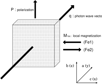
Figure 1: Geometry of absorption experiment.[5] X-rays propagate along the $a$ axis with polarization along the $b$ axis or the $c$ axis. The electric dipole moment is along the $b$ axis. When the magnetic field is applied to the positive direction of the $c$ axis, the sublattice magnetization is directed to the negative and positive directions of the $c$ axis at Fe1 sites and at Fe2 sites, respectively. When the magnetic field is reversed, the sublattice magnetization is reversed.

In the analysis of absorption spectra, we consider only the processes on Fe atoms, since the $1s$-core state is well localized on Fe atoms. In addition to the $E1$-$E1$ and $E2$-$E2$ processes, we formulate the $E1$-$E2$ interference process which gives rise to the magnetoelectric spectra. The contribution of this process arises from the mixing of the $3d^{6}\underline{1s}$-configuration to the $4p3d^{5}\underline{1s}$-configuration, where $\underline{1s}$ indicates the presence of a $1s$-core hole. Such mixings exist only under the noncentrosymmetric environment. In the present analysis, we describe the $E1$-$E2$ process by employing a cluster model of FeO₆, where all the $3d$ and $4p$ orbitals of Fe atoms and the 2p orbitals of O atoms as well as the Coulomb and the spin-orbit interactions in the $3d$ orbitals are taken into account. We obtain an effective hybridization between the $4p$ and $3d$ states in addition to the ligand field on the $3d$ states through the hybridization with the O $2p$ states. On the basis of these frameworks, we clarify various symmetry relations to the $E1$-$E2$ process and the relation between the nonreciprocal directional dichroism and the anapole moment. Furthermore, we numerically calculate the absorption spectra as a function of photon energy by diagonalizing the Hamiltonian matrix in the $3d^{6}$- and $4p3d^{5}$-configurations. The shapes of magnetoelectric spectra as a function of photon energy are found similar to the experimental curves but their signs are opposite to the experiment in the pre-$K$-edge region.[5] The origin for the opposite sign is not known. Note that the magnetoelectric spectra in the optical absorption have been obtained in agreement with the experiment by using the same cluster model.[8]

This paper is organized as follows. In §2, we introduce a cluster model of FeO₆. In §3, we describe the x-ray transition operators associated with Fe atoms. In §4, we derive the formulas of x-ray absorption, and present the calculated spectra in comparison with the experiment. The last section is devoted to concluding remarks.

2 Electronic Structures

2.1 FeO₆ cluster and $4p$ band

In a FeO₆ cluster, we consider the $1s$, $3d$ and $4p$ states in the Fe atom, and the $2p$ states in O atoms. The Hamiltonian may be written as

$$H = H^{3d}+H^{2p}+H_{\rm hyb}^{3d-2p}+H^{4p}+H_{\rm hyb}^{4p-2p}$$ (1)

$$+ H^{1s}+H^{1s-3d}+H^{1s-4p},$$

where

$$H^{3d} = \sum_{m\sigma}E_{m}^{d}d^{\dagger}_{m\sigma}d_{m\sigma}$$ (2)

$$+ \frac{1}{2}\sum_{\nu_{1}\nu_{2}\nu_{3}\nu_{4}}g\left(\nu_{1}\nu_{2};\nu_{3}\nu_{4}\right)d_{\nu_{1}}^{\dagger}d_{\nu_{2}}^{\dagger}d_{\nu_{4}}d_{\nu_{3}}$$

$$+ \zeta_{3d}\sum_{mm^{\prime}\sigma\sigma^{\prime}}\langle m\sigma|{\bf L}\cdot{\bf S}|m^{\prime}\sigma^{\prime}\rangle d^{\dagger}_{m\sigma}d_{m^{\prime}\sigma^{\prime}}$$

$$+ {\bf H}_{\rm xc}\cdot\sum_{m\sigma\sigma^{\prime}}({\bf S})_{\sigma\sigma^{\prime}}d^{\dagger}_{m\sigma}d_{m\sigma^{\prime}},$$

$$H^{2p} = \sum_{j\eta\sigma}E^{p}p^{\dagger}_{j\eta\sigma}p_{j\eta\sigma},$$ (3)

$$H_{\rm hyb}^{3d-2p} = \sum_{j\eta\sigma m}t_{m\eta}^{3d-2p}(j)d_{m\sigma}^{\dagger}p_{j\eta\sigma}+{\rm H.c.},$$ (4)

$$H^{4p} = \sum_{{\bf k}\eta^{\prime}\sigma}\epsilon_{4p}({\bf k})p^{\prime\dagger}_{{\bf k}\eta^{\prime}\sigma}p^{\prime}_{{\bf k}\eta^{\prime}\sigma},$$ (5)

$$H_{\rm hyb}^{4p-2p} = \sum_{j\eta\sigma\eta^{\prime}}t_{\eta^{\prime}\eta}^{4p-2p}(j)p^{\prime\dagger}_{\eta^{\prime}\sigma}p_{j\eta\sigma}+{\rm H.c.},$$ (6)

$$H^{1s} = \epsilon_{1s}\sum_{\sigma}s^{\dagger}_{\sigma}s_{\sigma},$$ (7)

$$H^{1s-3d} = U^{1s-3d}\sum_{m\sigma\sigma^{\prime}}d^{\dagger}_{m\sigma}d_{m\sigma}s^{\dagger}_{\sigma^{\prime}}s_{\sigma^{\prime}},$$ (8)

$$H^{1s-4p} = U^{1s-4p}\sum_{\eta^{\prime}\sigma\sigma^{\prime}}p^{\prime\dagger}_{\eta^{\prime}\sigma}p^{\prime}_{\eta^{\prime}\sigma}s^{\dagger}_{\sigma^{\prime}}s_{\sigma^{\prime}}.$$ (9)

The energy of $3d$ electrons can be described by $H^{3d}$ [eq. (2)] where $d_{m\sigma}$ represents an annihilation operator of a $3d$ electron with spin $\sigma$ and orbital $m$ ($=x^{2}-y^{2},3z^{2}-r^{2},yz,zx,xy$). The symbol $E_{m}^{d}$ refers to the energy of $3d$ state with orbital $m$. The second and third terms of eq. (2) represent the intra-atomic Coulomb and spin-orbit interactions for $3d$ electrons, respectively. The matrix elements $g\left(\nu_{1}\nu_{2};\nu_{3}\nu_{4}\right)$ are expressed in terms of the Slater integrals $F^{0}$, $F^{2}$, and $F^{4}$ [$\nu$ stands for $\left(m,\sigma\right)$], and the spin-orbit coupling is $\zeta_{3d}$. We evaluate atomic values of $F^{2}$, $F^{4}$ and $\zeta_{3d}$ within the Hartree-Fock (HF) approximation,[9] and multiply $0.8$ to these atomic values in order to take account of the slight screening effect. On the other hand, we multiply 0.25 to the atomic value for $F^{0}$, since $F^{0}$ is known to be considerably screened by solid-state effects. The last term in eq. (2) describes the energy arising from the exchange interaction with neighboring Fe atoms, where $({\bf S})_{\sigma\sigma^{\prime}}$ represents the matrix element of the spin operator of $3d$ electrons. The exchange field ${\bf H}_{\rm xc}$ has a dimension of energy, and is $\sim k_{\rm B}T_{c}/4$ with $T_{c}\sim 250$ K. Note that this term has merely a role of selecting the ground state by lifting the degeneracy and therefore the spectra depend little on its absolute value. The ${\bf H}_{\rm xc}$ is directed to the negative direction of the $c$ axis at Fe1 sites when the magnetic field is applied along the positive direction of the $c$ axis.

The energy of oxygen $2p$ electrons is given by $H^{2p}$ where $p_{j\eta\sigma}$ is the annihilation operator of the $2p$ state of energy $E^{p}$ with $\eta=x,y,z$ and spin $\sigma$ at the oxygen site $j$. The Coulomb interaction is neglected in oxygen 2p states. The $H^{3d-2p}_{\rm hyb}$ denotes the hybridization energy between the $3d$ and $2p$ states with the coupling constant $t_{m\eta}^{3d-2p}$. The energy of the $2p$ level relative to the $3d$ levels is determined from the charge-transfer energy $\Delta$ defined by $\Delta=E^{d}-E^{p}+15U(3d^{6})-10U(3d^{5})$ with $E^{d}$ being an average of $E_{m}^{d}$. The multiplet-averaged $d$-$d$ Coulomb interaction in the $3d^{6}$ and $3d^{5}$ configurations are referred to as $U(3d^{6})$ and $U(3d^{5})$, respectively, which are defined by $U=F^{0}-\left(2/63\right)F^{2}-\left(2/63\right)F^{4}$.

The $H^{4p}$ represents the energy of the $4p$ states, where $p^{\prime}_{{\bf k}\eta^{\prime}\sigma}$ is the annihilation operator of the $4p$ state with momentum ${\bf k}$, $\eta^{\prime}=x,y,z$, and spin $\sigma$. The $4p$ states form an energy band $\epsilon_{4p}({\bf k})$. The density of states (DOS) of the $4p$ band is inferred from the $K$-edge absorption spectra[5] (see Fig. 2). The $H^{4p-2p}_{\rm hyb}$ represents the hybridization between the $4p$ and oxygen $2p$ states with the coupling constant $t_{\eta^{\prime}\eta}^{4p-2p}$. The annihilation operator of the local $4p$ orbital $p^{\prime}_{\eta^{\prime}\sigma}$ may be expressed as $p^{\prime}_{\eta^{\prime}\sigma}=(1/\sqrt{N_{0}})\sum_{\bf k}p^{\prime}_{{\bf k}\eta^{\prime}\sigma}$ ($N_{0}$ is the discretized number of ${\bf k}$-points).

The energy of the $1s$ state is denoted as $H^{1s}$ where $s_{\sigma}$ represents the annihilation operator of the $1s$ state with spin $\sigma$. Finally, the interaction between the $1s$ and $3d$ states and that between the $1s$ and $4p$ states are denoted as $H^{1s-3d}$ and $H^{1s-4p}$, respectively.

Table 1 lists the parameter values used in this paper, which are used in our previous paper analyzing the optical spectra in GaFeO₃,[8] and are consistent with the values in previous calculations for Fe₃O₄.[10, 11]

Table 1: Parameter values for a FeO₆ cluster in the $3d^{5}$ configuration, in units of eV. The Slater-Koster two-center integrals are defined for the Fe atom at the center of the octahedron.

$F^{0}(3d,3d)$	6.39	$(pd\sigma)_{2p,3d}$	-1.9
$F^{2}(3d,3d)$	9.64	$(pd\pi)_{2p,3d}$	0.82
$F^{4}(3d,3d)$	6.03	$(pp\sigma)_{2p,4p}$	3.5
$\zeta_{3d}$	0.059	$(pp\pi)_{2p,4p}$	-1.0
$\Delta$	3.3

2.2 Ligand field and effective hybridization between the $4p$ and $3d$ states

Fe atoms are assumed to be displaced from the center of the octahedron along the $b$ axis. The shift $\delta$ is $0.26\textrm{\AA}$ at Fe1 sites and $-0.11\textrm{\AA}$ at Fe2 sites. We evaluate the hybridization matrices $t^{3d-2p}_{m\eta}(j)$ and $t^{4p-2p}_{\eta^{\prime}\eta}(j)$ for the Fe atom at the off-center positions by modifying the Slater-Koster two-center integrals for the Fe atom at the central position of the octahedron (Table 1) with the assumption that $(pd\sigma)_{2p,3d}$, $(pd\pi)_{2p,3d}\propto d^{-4}$, and $(pp\sigma)_{4p,2p}$, $(pp\pi)_{4p,2p}\propto d^{-2}$ for $d$ being the Fe-O distance.[12] Thereby the ligand field Hamiltonian on the $3d$ states is given in second-order perturbation theory,

$$\tilde{H}^{3d-3d}=\sum_{mm^{\prime}\sigma}\tilde{t}_{mm^{\prime}}^{3d-3d}d_{m\sigma}^{\dagger}d_{m^{\prime}\sigma}+{\rm H.c.},$$ (10)

with

$$\tilde{t}^{3d-3d}_{mm^{\prime}}=\sum_{j\eta}t^{3d-2p}_{m\eta}(j)t^{3d-2p}_{m^{\prime}\eta}(j)/\Delta,$$ (11)

where the sum over $j$ is taken on neighboring O sites, and $\Delta=3.3$ eV is the charge transfer energy defined in §2.1. In addition to the ligand field corresponding to the cubic symmetry, we have a field proportional to $\delta^{2}$. The latter causes extra splittings of the $3d$ levels. Similarly, we can evaluate the effective hybridization between the $4p$ and $3d$ states in the form:

$$\tilde{H}^{4p-3d}=\sum_{\eta^{\prime}m\sigma}\tilde{t}_{\eta^{\prime}m}^{4p-3d}p^{\prime\dagger}_{\eta^{\prime}\sigma}d_{m\sigma}+{\rm H.c.}$$ (12)

Here, the effective coupling is defined by

$$\tilde{t}^{4p-3d}_{\eta^{\prime}m}=\sum_{j\eta}t^{4p-2p}_{\eta^{\prime}\eta}(j)t^{3d-2p}_{m\eta}(j)/(E^{4p}-E^{2p}),$$ (13)

where $E^{4p}$ is the average of the $4p$-band energy, which is estimated as $E^{4p}-E^{2p}\approx 17$ eV. The value of coupling coefficient $\tilde{t}^{4p-3d}_{\eta^{\prime}m}$ is nearly proportional to the shift $\delta$ of the Fe atom from the center of the octahedron.

2.3 Ground state

We assume that Fe ions are in the $d^{5}$-configuration in the ground state, which will be denoted as $|\Phi_{g}(d^{5})\rangle$ with eigenenergy $E_{g}(d^{5})$. We calculate the state by diagonalizing the Hamiltonian $H_{3d}+\tilde{H}^{3d-3d}$, where the exchange field ${\bf H}_{\textrm{xc}}$ and the displacement of Fe atoms from the center of the octahadron are different from Fe1 and Fe2 sites. The lowest energy state is characterized as ${}^{6}A_{1}$ under the trigonal crystal field when the exchange field and the spin-orbit interaction are disregarded. The inclusion of these interactions could induce the orbital moment $\hbar\langle L_{x}\rangle$, but its absolute value is given less than $0.004\hbar$.

3 Absorption process on Fe

The interaction between the electromagnetic wave and electrons is described by

$$H_{\rm int}=-\frac{1}{c}\int{\bf j}({\bf r})\cdot{\bf A}({\bf r}){\rm d}^{3}{\bf r},$$ (14)

where $c$ stands for the speed of light and ${\bf j}$ represents the current-density operator. The electromagnetic field ${\bf A}({\bf r})$ for linear polarization is defined as

$${\bf A}({\bf r})=\sum_{\bf q}\sqrt{\frac{2\pi\hbar^{2}c^{2}}{V\hbar\omega_{\bf q}}}{\bf e}c_{\bf q}{\rm e}^{i\textbf{q}\cdot\textbf{r}}+{\rm H.c.},$$ (15)

where $c_{\bf q}$ and $\hbar\omega_{\bf q}$ are the annihilation operator and the energy of photon, respectively. The unit vector of polarization is described by ${\bf e}$. We approximate this expression into a sum of the contributions from each Fe atom:

$$H_{\rm int}=-\frac{1}{c}\sum_{{\bf q},i}{\bf j}({\bf q},i)\cdot{\bf A}({\bf q},{\bf e},i)+{\rm H.c.},$$ (16)

with

$${\bf j}({\bf q},i) = \sum_{nn^{\prime}}\left[\int{\rm e}^{i{\bf q}\cdot({\bf r}-{\bf r}_{i})}{\bf j}_{nn^{\prime}}({\bf r}-{\bf r}_{i}){\rm d}^{3}({\bf r}-{\bf r}_{i})\right]a_{n}^{\dagger}(i)a_{n^{\prime}}(i),$$ (17)

$${\bf A}({\bf q},{\bf e},i) = \sqrt{\frac{2\pi\hbar c^{2}}{V\omega_{\bf q}}}{\bf e}c_{\bf q}{\rm e}^{i\textbf{q}\cdot\textbf{r}_{i}}.$$ (18)

The local current operator may be described by[13]

$${\bf j}_{nn^{\prime}}({\bf r}-{\bf r}_{i}) = \frac{ie\hbar}{2m}\big{[}(\nabla\phi^{*}_{n})\phi_{n^{\prime}}-\phi_{n}^{*}\nabla\phi_{n^{\prime}}\big{]}$$

$$- \frac{e^{2}}{mc}{\bf A}\phi_{n}^{*}\phi_{n^{\prime}}+\frac{e\hbar}{mc}c\nabla\times[\phi_{n}^{*}{\bf S}\phi_{n^{\prime}}].$$

The integration in eq. (17) is carried out around site $i$, and $a_{n}(i)$ is the annihilation operator of electron with the local orbital expressed by the wave function $\phi_{n}({\bf r}-{\bf r}_{i})$. The charge and the mass of electron are denoted as $e$ and $m$, and $\hbar{\bf S}$ is the spin operator of electron. The second term in eq. (LABEL:eq.current), which describes the scattering of photon, will be neglected in the following. The approximation made by taking account of the process only on Fe atoms may be justified at the core-level spectra, since the core state is well localized at Fe sites.

The absorption experiment[5] we analyse has been carried out on the geometry that the photon propagates along the $a$-axis with linear polarization, as illustrated in Fig. 1. Corresponding to this situation, it is convenient to rewrite the interaction between the matter and the photon in a form,

$$H_{\rm int}=-e\sum_{\bf q}\sqrt{\frac{2\pi}{V\hbar\omega_{\bf q}}}\sum_{i}T({\bf q},{\bf e},i)c_{\bf q}{\rm e}^{i\textbf{q}\cdot\textbf{r}_{i}}+{\rm H.c.},$$ (20)

where the transition operator $T({\bf q},{\bf e},i)$ is defined as $\hbar\textbf{e}\cdot\textbf{j}(\textbf{q},i)/e$. The explicit expression of $T({\bf q},{\bf e},i)$ for the $E$1 and $E$2 transitions are given in the following subsections.

3.1 $E1$ transition

The transition operator $T({\bf q},{\bf e},i)$ for the $E1$ transition is obtained by putting ${\rm e}^{i{\bf q}\cdot({\bf r}-{\bf r}_{j})}=1$ in eq. (17). Therefore it is independent of the propagation direction of photon. For the polarization along the z-axis, the first term in eq. (LABEL:eq.current) is rewritten by employing the following relation

$$\int\phi_{n}^{*}\frac{\partial}{\partial z}\phi_{n^{\prime}}{\rm d}^{3}{\bf r}=-\frac{m}{\hbar^{2}}(\epsilon_{n}-\epsilon_{n^{\prime}})\int\phi_{n}^{*}z\phi_{n^{\prime}}{\rm d}^{3}{\bf r},$$ (21)

where $\epsilon_{n}$ and $\epsilon_{n^{\prime}}$ are energy eigenvalues corresponding to the eigenstates $\phi_{n}$ and $\phi_{n^{\prime}}$, respectively. At the $K$-edge, we assign the $4p$ states to $\phi_{n}$ and $1s$ state to $\phi_{n^{\prime}}$. Hence the transition operator $T^{E1}$ is expressed as

$$T^{E1}({\bf q},{\bf e},i)=iB^{E1}\sum_{i\sigma}N^{E1}_{\eta}[p^{\prime\dagger}_{\eta\sigma}(i)s_{\sigma}(i)-s^{\dagger}_{\sigma}(i)p^{\prime}_{\eta\sigma}(i)].$$ (22)

where $i$ runs over Fe sites. Non-vanishing values of the coefficients $N^{E1}_{\eta}$’s are given by $N_{\eta}=1/\sqrt{3}$ for the polarization along the $\eta$ $(=x,y,z)$ axis, independent of the propagating direction of photon. The coefficient $B^{E1}$ is defined by

$$B^{E1}=(\epsilon_{4p}-\epsilon_{1s})\int_{0}^{\infty}r^{3}R_{4p}(r)R_{1s}(r){\rm d}r,$$ (23)

where $R_{1s}(r)$ and $R_{4p}(r)$ are radial wave functions of the $1s$ and $4p$ states with energy $\epsilon_{1s}$ and $\epsilon_{4p}$, respectively, in the Fe atom. The energy difference may be approximate as $\epsilon_{4p}-\epsilon_{1s}\sim\hbar\omega_{\bf q}=\hbar cq$. [11] Within the HF approximation $B^{E1}$ is estimated as $B^{E1}\approx 1.5\times 10^{-7}{\rm cm\cdot eV}$ in the 1s²3d⁵4p^0.001-configuration of an Fe atom.[9]

3.2 $E2$ transition

The transition operator for the $E2$ transition is extracted from eq.  (17) by retaining the second term in the expansion ${\rm e}^{i{\bf q}\cdot({\bf r}-{\bf r}_{i})}\approx 1+i{\bf q}\cdot({\bf r}-{\bf r}_{i})+\cdots$. Let the photon be propagating along the $y$-axis with the polarization parallel to the $z$-axis. Then we could derive a relation,

$$\int\phi_{n}^{*}y\frac{\partial}{\partial z}\phi_{n^{\prime}}{\rm d}^{3}{\bf r} = -\frac{m}{\hbar^{2}}(\epsilon_{n}-\epsilon_{n^{\prime}})\int\phi_{n}^{*}\frac{yz}{2}\phi_{n^{\prime}}{\rm d}^{3}{\bf r}$$ (24)

$$+ \frac{i}{2}\int\phi_{n}^{*}L_{x}\phi_{n^{\prime}}{\rm d}^{3}{\bf r},$$

where $\hbar L_{x}$ is the orbital angular momentum operator. The last term should be moved into the terms of the $M1$ transition. [8] At the $K$-edge, we assign the $3d$ states to $\phi_{n}$ and the $1s$ state to $\phi_{n^{\prime}}$, respectively. Hence the transition operator $T^{E2}$ may be expressed as

$$T^{E2}({\bf q},{\bf e},i)=-qB^{E2}\sum_{im\sigma}N^{E2}_{m}({\bf q})[d^{\dagger}_{m\sigma}(i)s_{\sigma}(i)-s^{\dagger}_{\sigma}(i)d_{m\sigma}(i)].$$ (25)

When the photon is propagating along the $y$-axis, $m$ is selectively $yz$ with $N^{E2}_{yz}({\bf q})=1/(2\sqrt{15})$ in the polarization along the $z$-axis, and $m$ is selectively $xy$ with $N^{E2}_{xy}({\bf q})=1/(2\sqrt{15})$ in the polarization along the $x$-axis, respectively. Note that a relation $N_{m}^{E2}(-\textbf{q})=-N_{m}^{E2}(\textbf{q})$ holds. The $B^{E2}$ are defined by

$$B^{E2}=(\epsilon_{3d}-\epsilon_{1s})\int_{0}^{\infty}r^{4}R_{3d}(r)R_{1s}(r){\rm d}r,$$ (26)

where $R_{3d}(r)$ is radial wave function of the $3d$ state with energy $\epsilon_{3d}$ in the Fe atom. An evaluation within the HF approximation gives $B^{E2}\approx 1.7\times 10^{-16}$cm${}^{2}\cdot$eV.[9]

4 Absorption spectra

Restricting the processes on Fe atoms, we sum up cross sections at Fe sites to obtain the absorption intensity $I(\omega_{\bf q},{\bf e})$. Dividing it by the incident flux $c/V$, we have

$$I(\omega_{\bf q},{\bf e}) \propto \frac{4\pi^{2}e^{2}}{\hbar^{2}c\omega_{\bf q}}\sum_{i}\sum_{f}|\langle\Psi_{f}(i)|T({\bf q},{\bf e},i)|\Psi_{g}(i)\rangle|^{2}$$ (27)

$$\times\delta(\hbar\omega_{\bf q}+E_{g}-E_{f}),$$

where $T({\bf q},{\bf e},i)=T^{E1}({\bf q},{\bf e},i)+T^{E2}({\bf q},{\bf e},i)$, and $|\Psi_{g}(i)\rangle$ and $|\Psi_{f}(i)\rangle$ represent the ground and the final states with energy $E_{g}$ and $E_{f}$ at site $i$, respectively. The sum over $f$ is taken over all the excited state at Fe sites.

In the Fe pre-K-edge region, the final states are constructed by perturbation theory starting from the states ($|\Phi_{m}(d^{6}),\underline{1s\sigma}\rangle$) in the $d^{6}$ configuration with the $1s$-core hole. Within the second-order perturbation of $\tilde{H}^{4p-3d}$, they are given by

$$|\Psi_{f}(i)\rangle = |\Phi_{m}(d^{6}),\underline{1s\sigma}\rangle$$ (28)

$$+ \sum_{n{\bf k}\eta^{\prime}}|\Phi_{n}(d^{5}),{\bf k}\eta^{\prime}\sigma,\underline{1s\sigma}\rangle\frac{1}{E_{f}-E^{\prime}_{n{\bf k}\eta^{\prime}}}$$

$$\times \langle\Phi_{n}(d^{5}),{\bf k}\eta^{\prime}\sigma,\underline{1s\sigma}|\tilde{H}^{4p-3d}|\Phi_{m}(d^{6}),\underline{1s\sigma}\rangle,$$

where $E_{f}$ stands for the energy of the unperturbed state. It is defined as

$$E_{f}=E_{m}(d^{6})-\epsilon_{1s}-E_{\rm int}(1s-d^{6}),$$ (29)

where $E_{\rm int}(1s-d^{6})$ is the interaction energy between the electron in the $1s$ states and electrons in the $3d^{6}$ configuration. In the second term of eq. (28), $E^{\prime}_{n{\bf k}\eta^{\prime}}$ is defined as

$$E^{\prime}_{n{\bf k}\eta^{\prime}}=E_{n}(d^{5})-\epsilon_{1s}+\epsilon_{4p}({\bf k})-E_{\rm int}(1s-4pd^{5}),$$ (30)

where $E_{\rm int}(1s-4pd^{5})$ is the interaction energy between the electron in the $1s$ states and electrons in the $4p3d^{5}$ configuration. Symbols ${\bf k}\eta^{\prime}\sigma$ and $\underline{1s\sigma}$ appeared in the bras and kets indicate the presence of an electron in the $4p$ state $({\bf k}\eta^{\prime}\sigma)$ and the absence of a $1s$-core electron with spin $\sigma$, respectively. Since the second term of eq. (28) is completely evaluated by $|\Phi_{m}(d^{6}),\underline{1s\sigma}\rangle$ and $E_{f}$, the label $f$ is specified by the $m$-th eigenstates of the $d^{6}$ configuration and the core-hole spin $\sigma$. Notice that the lowest values of eqs. (29) and (30) correspond to the positions of the pre- and main-edges, respectively.

The sum over ${\bf k}$ may be replaced by the integral with the help of the $4p$ DOS. In our numerical treatment, the position of the pre-edge energy is adjusted to the experimental value and the difference between the pre- and main-edges is chosen as the minimum of $E^{\prime}_{n{\bf k}\eta^{\prime}}$ to be $12$ eV higher than $E_{g}(d^{6})-\epsilon_{1s}-E_{\rm int}(1s-d^{6})$. For simplicity, the explicit dependence on site $i$ is omitted from the right hand side of eq. (28). From these wave-functions, we obtain the expression of transition amplitudes at site $i$ by

$$M({\bf q},{\bf e},i;f)=M^{E1}({\bf q},{\bf e},i;f)+M^{E2}({\bf q},{\bf e},i;f),$$ (31)

with

$$M^{E1}({\bf q},{\bf e},i;f) \equiv \langle\Psi_{f}(i)|T^{E1}({\bf q},{\bf e},i)|\Psi_{g}(i)\rangle$$ (32)

$$= \sum_{n{\bf k}\eta^{\prime}}\langle\Phi_{m}(d^{6}),\underline{1s\sigma}|\tilde{H}^{4p-3d}|\Phi_{n}(d^{5}),{\bf k}\eta^{\prime}\sigma,\underline{1s\sigma}\rangle$$

$$\times \frac{1}{E_{f}-E^{\prime}_{n{\bf k}\eta^{\prime}}}\langle\Phi_{n}(d^{5}),{\bf k}\eta^{\prime}\sigma,\underline{1s\sigma}|T^{E1}({\bf q},{\bf e},i)|\Phi_{g}(d^{5})\rangle,$$

$$M^{E2}({\bf q},{\bf e},i;f) \equiv \langle\Psi_{f}(i)|T^{E2}({\bf q},{\bf e},i)|\Psi_{g}(i)\rangle$$ (33)

$$= \langle\Phi_{m}(d^{6}),\underline{1s\sigma}|T^{E2}({\bf q},{\bf e},i)|\Phi_{g}(d^{5})\rangle.$$

With these amplitudes, eq. (27) is rewritten as

$$I(\omega_{\bf q},{\bf q},{\bf e}) \propto \frac{1}{\hbar\omega_{\bf q}}\sum_{i}\sum_{f}|M({\bf q},{\bf e},i;f)|^{2}$$ (34)

$$\times \frac{\Gamma/\pi}{[\hbar\omega_{\bf q}+E_{g}(d^{5})-E_{f}]^{2}+\Gamma^{2}},$$

where the $\delta$-function is replaced by the Lorentzian function with the life-time broadening width of $1s$-core hole $\Gamma=0.8$ eV.

Now we examine the symmetry relation of the amplitudes. First, let the propagating direction of photon be reversed with keeping other conditions. In eq. (17), $i{\bf q}\cdot({\bf r}-{\bf r}_{i})$ is to be replaced by $-i{\bf q}\cdot({\bf r}-{\bf r}_{i})$. We know that $N_{\eta}^{E1}$ has no dependence on q and that $N_{m}^{E2}(-\textbf{q})$ is equal to $-N_{m}^{E2}(\textbf{q})$. Since other conditions are the same, we have the new amplitudes $(M^{E1})^{\prime}=M^{E1}$ and $(M^{E2})^{\prime}=-M^{E2}$. Second, let the local magnetic moment at each Fe atom be reversed with keeping the same shifts from the center of octahedron. The reverse of the local magnetic moment corresponds to taking the complex conjugate of the wave functions. Considering eq. (32) together with eq. (22), we have $(M^{E1})^{\prime}=-(M^{E1})^{*}$. Similarly, considering eq. (33) together with eq. (25), we have $(M^{E2})^{\prime}=(M^{E2})^{*}$. Third, let the shifts of Fe atoms from the center of octahedron be reversed with keeping the same local magnetic moment, which means the reversal of the direction of the local electric dipole moment. This operation causes the reversal of the sign of $\tilde{H}^{4p-3d}$. However, no change is brought about to the $3d$ states in the $3d^{5}$- and $3d^{6}$-configurations, because the ligand field $\tilde{H}^{3d-3d}$ varies as $\delta^{2}$. As a result, we have the new amplitude $(M^{E1})^{\prime}=-M^{E1}$ from eq. (22) while $(M^{E2})^{\prime}=M^{E2}$.

As already stated, the direction of the local magnetic moment could be reversed by reversing the direction of the applied magnetic field, since the actual material is a ferrimagnet with slightly deviating from a perfect antiferromagnet. Let $I_{\pm}(\omega_{\bf q},{\bf q},{\bf e})$ be the intensity for the external magnetic field along the $\pm c$ axis. Then, from the second symmetry relation mentioned above, we have the average and the difference of the intensities as

$$\bar{I}(\omega_{\bf q},{\bf q},{\bf e}) \equiv \frac{1}{2}\left[I_{+}(\omega_{\bf q},{\bf q},{\bf e})+I_{-}(\omega_{\bf q},{\bf q},{\bf e})\right]$$ (35)

$$\propto \frac{1}{\hbar\omega_{\bf q}}\Biggl{\{}\sum_{i}\sum_{f}\Bigl{[}|M^{E1}({\bf q},{\bf e},i;f)|^{2}+|M^{E2}({\bf q},{\bf e},i;f)|^{2}\Bigr{]}$$

$$\times \frac{\Gamma/\pi}{[\hbar\omega_{\bf q}+E_{g}(d^{5})-E_{f}]^{2}+\Gamma^{2}}$$

$$+ \sum_{i}|B^{E1}|^{2}\frac{2}{3}\sum_{\bf k}\frac{\Gamma/\pi}{[\hbar\omega_{\bf q}+E_{g}(d^{5})-E^{\prime}_{g{\bf k}\eta}]^{2}+{\Gamma}^{2}}\Biggr{\}},$$

and

$$\Delta I(\omega_{\bf q},{\bf q},{\bf e}) \equiv I_{+}(\omega_{\bf q},{\bf q},{\bf e})-I_{-}(\omega_{\bf q},{\bf q},{\bf e})$$ (36)

$$\propto \frac{2}{\hbar\omega_{\bf q}}\sum_{i}\sum_{f}\Biggl{\{}\left[M^{E1}({\bf q},{\bf e},i;f)\right]^{*}M^{E2}({\bf q},{\bf e},i;f)$$

$$+ \left[M^{E2}({\bf q},{\bf e},i;f)\right]^{*}M^{E1}({\bf q},{\bf e},i;f)\Biggr{\}}$$

$$\times \frac{\Gamma/\pi}{[\hbar\omega_{\bf q}+E_{g}(d^{5})-E_{f}]^{2}+\Gamma^{2}},$$

respectively. The $M^{E1}$ and $M^{E2}$ represent the amplitudes when the magnetic field is applied parallel to the $c$ axis. For the average intensity [eq. (35)], the last term describes the $K$-edge spectra due to the $E1$ transition that the $1s$ electron is excited to the $4p$ band. Although its main contribution is restricted in the main $K$-edge region, its tail spreads over the pre-$K$-edge spectra due to the life-time width. We see that the difference intensity [eq. (36)] is brought about from the $E1$-$E2$ interference process. According to the symmetry relations mentioned above, it is expected to follow[5]

$$\Delta I(\omega_{\bf q},{\bf q},{\bf e})\propto{\bf q}\cdot\sum_{i}{\bf P}_{\rm loc}(i)\times{\bf M}_{\rm loc}(i),$$ (37)

where ${\bf P}_{\rm loc}(i)$ and ${\bf M}_{\rm loc}(i)$ are the electric and the magnetic dipole moment of Fe atom at site $i$, respectively. Note that ${\bf P}_{\rm loc}(i)$ is proportional to $\boldsymbol{\delta}_{i}[\equiv(0,0,\delta)]$. Then, the right hand side of eq. (37) is the sum of the local toroidal moment $\boldsymbol{\tau}(i)$ [$\equiv\boldsymbol{\delta}_{i}\times{\bf M}_{\rm loc}(i)$]. [14] We have already derived the same form in the optical absorption spectra,[8] which is brought about by the $E1$-$M1$ interference process. The spectra change their sign if one of the vectors among ${\bf q}$, ${\bf P}_{\rm loc}$, or ${\bf M}_{\rm loc}$ reverses its direction.

Figure 2 shows the calculated average intensity $\overline{I}(\omega_{\bf q},{\bf q},{\bf e})$ as a function of photon energy $\hbar\omega_{\bf q}$, in comparison with the experiment.[5] The $1s$-core energy is adjusted such that the $K$-edge position corresponds to the experiment. The intensity at the $K$-edge ($\hbar\omega_{\bf q}>7120$ eV) mainly comes from the $E1$-$E1$ process given by the last term of eq. (35). In the pre-$K$-edge region ($\hbar\omega_{\bf q}\sim 7110-7115$ eV), the tail of that intensity spreads due to the life-time broadening of the core level. In addition, we have another contribution of $E1$-$E1$ process through the term proportional to $|M^{E1}|^{2}$, and that of the $E2$-$E2$ process through the term proportional to $|M^{E2}|^{2}$. The latter is found larger than the former, giving rise to a small two-peak structure with a weak polarization dependence (the inset in Fig. 2). The $E1$-$E1$ process through the term proportional to $|M^{E1}|^{2}$ is effective only on the noncentrosymmetric situation, because the $4p3d^{5}\underline{1s}$-configuration has to mix with the $3d^{6}\underline{1s}$-configuration. Note that the $E1$-$E1$ process could also gives rise to the intensity in the pre-$K$-edge region through the mixing of the $4p$ state with the $3d$ states at neighboring Fe sites. This process need not the noncentrosymmetric situation, and has nothing to do with the magnetoelectric spectra. It is known that a substantial intensity of the resonant x-ray scattering (RXS) spectra is brought about from this process at the pre-$K$-edge on LaMnO₃,[15] but the present analysis could not include this process because of the cluster size.

Figure 2: Average intensity $\overline{I}(\omega_{\bf q},{\bf q},{\bf e})$ as a function of photon energy $\hbar\omega_{\bf q}$. Photons propagate along the positive direction of the $a$ axis with polarization vector ${\bf e}$ along the $b$ axis. The solid line represents the calculated spectra. The broken line denotes the experimental data with the background intensity subtracted from the raw data given in ref. [Jung2004]. The dotted line represents the $4p$DOS; both the low-energy and high-energy sides are arbitrarily cut-off.

Figure 3 shows the magnetoelectric spectra $\Delta I(\omega_{\bf q},{\bf q},{\bf e})$ as a function of photon energy $\hbar\omega_{\bf q}$. For polarization ${\bf e}$ parallel to the $b$ axis, the calculated spectra form a positive sharp peak and then change into a negative double peak with increasing $\hbar\omega_{\bf q}$. On the other hand, for polarization ${\bf e}$ parallel to the $c$ axis, the calculated spectra form a negative sharp peak and then change into a positive sharp peak with increasing $\hbar\omega_{\bf q}$. The corresponding experimental curves look similar, but their signs are opposite to the calculated ones. We do not find the origin for the opposite sign.

Figure 3: Difference of the absorption intensities $\Delta I(\omega_{\bf q},{\bf q},{\bf e})$ as a function of photon energy $\hbar\omega_{\bf q}$ when the magnetic field is applied parallel and antiparallel to the $c$ axis. The solid and broken lines correspond to $\Delta I(\omega_{\bf q},{\bf q},{\bf e})$ where photons propagate along the positive direction of the $a$ axis with polarization vector ${\bf e}$ along the $b$ and $c$ axes, respectively. Experimental data are taken from ref. [Jung2004] and denoted as filled ($\textbf{e}\parallel b$) and open ($\textbf{e}\parallel c$) circles, respectively.

5 Concluding Remarks

We have studied the magnetoelectric effects on the x-ray absorption spectra in a polar ferrimagnet GaFeO₃. We have performed a microscopic calculation of the absorption spectra using a cluster model of FeO₆. The cluster consists of an octahedron of O atoms and an Fe atom displaced from the center of octahedron. We have disregarded additional small distortions of the octahedron. We have derived an effective hybridization between the $4p$ and $3d$ states as well as the ligand field on the $3d$ states by modifying the Fe-O hybridizations due to the shifts of Fe atoms. This leads to the mixing of the $4p3d^{5}$-configuration to the $3d^{6}$-configuration, and thereby to finite contributions of the $E1$-$E2$ interference process to the magnetoelectric spectra. We have derived the symmetry relations of the amplitudes $M^{E1}$ and $M^{E2}$, and have discussed the directional dichroism of the spectra. The cluster model used in the present paper is the same as the model used in the analysis of the optical absorption spectra in GeFeO₃ and is similar to the model used in the analysis of RXS in Fe₃O₄.[11] We have numerically calculated the magnetoelectric spectra as a function of photon energy in the pre-$K$-edge region. Although the spectral shapes are similar to the experimental curves, their signs are opposite to the experimental ones. The origin for the opposite sign has not been clarified yet. We would like to simply comment that the magnetoelectric spectra in the optical absorption are obtained in agreement with the experiment by using the same model.[8]

The magnetoelectric effect on RXS has been studied experimentally[16] and theoretically[17, 18] in GaFeO₃. We think the approach used in the present paper is effective also to the analysis of RXS. Closely related to these studies, the magnetoelectric effects on RXS have also been measured,[19, 20] and theoretically analyzed[11] in magnetite, where A sites are tetrahedrally surrounded by oxygens with the local inversion symmetry being broken.

References

• [1] J. P. Remeika: J. Appl. Phys. 31 (1960) S263.
• [2] G. T. Rado: Phys. Rev. Lett. 13 (1964) 335.
• [3] T. Arima, D. Higashiyama, Y. Kaneko, J. P. He, T. Goto, S. Miyasaka, T. Kimura, K. Oikawa, T. Kamiyama, R. Kumai, and Y. Tokura : Phys. Rev. B 70 (2004) 064426.
• [4] J. H. Jung, M. Matsubara, T. Arima, J. P. He, Y. Kaneko, and Y. Tokura: Phys. Rev. Lett. 93 (2004) 037403.
• [5] M. Kubota, T. Arima, Y. Kaneko, J. P. He, X. Z. Yu, and Y. Tokura: Phys. Rev. Lett. 92 (2004) 137401.
• [6] E. A. Wood: Acta Crystallogr. 13 (1960) 682.
• [7] R. B. Frankel, N. A. Blum, S. Foner, A. J. Freeman, and M. Schieber: Phys. Rev. Lett. 15 (1965) 958.
• [8] J. Igarashi and T. Nagao: Phys. Rev. B 80 (2009) 054418.
• [9] R. Cowan: The Theory of Atomic Structure and Spectra (University of California,Berkeley,1981).
• [10] J. Chen, D. J. Huang, A. Tanaka, C. F. Chang, S. C. Chung, W. B. Wu, and C. T. Chen : Phys. Rev. B 69 (2004) 085107.
• [11] J. Igarashi and T. Nagao : J. Phys. Soc. Jpn. 77 (2008) 084706.
• [12] W. A. Harrison: Elementary Electronic Structure (World Scientific,Singapore,2004).
• [13] L. D. Landau and E. M. Lifshitz: Quantum Mechanics (Pergamon,Oxford,1977).
• [14] Y. F. Popov, A. M. Kadomtseva, G. P. Vorob’ev, V. A. Timofeeva, D. M. Ustinin, A. K. Zvezdin, and M. M. Tegeranchi : Zh. Eksp. Teor. Fiz. 114 (1998) 263 [Translation: Sov. Phys. JETP 87 (1998) 146].
• [15] M. Takahashi, J. Igarashi, and P. Fulde : J. Phys. Soc. Jpn. 69 (2000) 1614.
• [16] T. Arima, J. H. Jung, M. Matsubara, M. Kubota, J. P. He, Y. Kaneko, and Y. Tokura : J. Phys. Soc. Jpn. 74 (2005) 1419.
• [17] S. Di Matteo and Y. Joly : Phys. Rev. B 74 (2006) 014403.
• [18] S. W. Lovesey, K. S. Knight, and E. Balcar : J. Phys.:Condens. Matter 19 (2007) 376205.
• [19] M. Matsubara, Y. Shimada, T. Arima, Y. Taguchi, and Y. Tokura : Phys. Rev. B 72 (2005) 220404(R).
• [20] M. Matsubara, Y.Kaneko, J. P. He, H. Okamoto, and Y. Tokura : Phys. Rev. B 79 (2009) 140411(R).