Theory and Applications of Coulomb Excitation

Abstract

Because the interaction is well-known, Coulomb excitation is one of the best tools for the investigation of nuclear properties. In the last 3 decades new reaction theories for Coulomb excitation have been developed such as: (a) relativistic Coulomb excitation, (b) Coulomb excitation at intermediate energies, and (c) multistep coupling in the continuum. These developments are timely with the advent of rare isotope facilities. Of special interest is the Coulomb excitation and dissociation of weakly-bound systems. I review the Coulomb excitation theory, from low to relativistic collision energies. Several applications of the theory to situations of interest in nuclear physics and nuclear astrophysics are discussed.

Lecture notes presented at the 8th CNS-EFES Summer School, held at Center for Nuclear Study (CNS), the University of Tokyo, and at the RIKEN Wako Campus, August 26 - September 1, 2009. Supported by the Japan-US Theory Institute for Physics with Exotic Nuclei (JUSTIPEN).

“I don’t know what they have to say,
It makes no difference anyway –
Whatever it is, I’m against it! ” - Groucho Marx

I What is Coulomb excitation?

Coulomb excitation is a process of inelastic scattering in which a charged particle transmits energy to the nucleus through the electromagnetic field. This process can happen at a much lower energy than the necessary for the particle to overcome the Coulomb barrier; the nuclear force is, in this way, excluded in the process.

Let $v$ be the relative velocity of two nuclei at infinity which determines the energy of relative motion $E=mv^{2}/2$ where $m$ is the reduced mass. The strength of Coulomb interaction can be measured by the Sommerfeld parameter

$$\eta=\frac{Z_{1}Z_{2}e^{2}}{\hbar v}$$ (1)

where $Z_{1,2}$ are charges of the nuclei. For $Z_{1}Z_{2}>137$, or $v\ll c$, the parameter (1) can easily reach values $\eta\gg 1$.

This situation allows for the use of the semiclassical approximation: the Coulomb interaction is taken into account exactly in determining the classical Rutherford trajectory of relative motion ${\bf R}(t)$ where ${\bf R}$ is the distance between the centers of the colliding nuclei, Fig. 1. The relative energy $E$ is assumed to be large enough so that we can neglect the feedback from the intrinsic excitations to relative motion. Then the trajectory is fixed by energy and impact parameter or deflection angle.

The classical distance of closest approach,

$$a=2a_{0}={2Z_{1}Z_{2}e^{2}\over mv^{2}}$$ (2)

is larger than $R_{1}+R_{2}$ at relative energy lower than the Coulomb barrier

$$E_{B}=\frac{Z_{1}Z_{2}e^{2}}{R_{1}+R_{2}}.$$ (3)

The excitation is generated by the time-dependent field and the probability of the process is determined by the presence in this field of Fourier harmonics with the excitation frequencies

$$\omega={E_{f}-E_{i}\over\hbar}.$$ (4)

If the motion is too slow, the field acts adiabatically, the intrinsic wave function is changing reversibly and the probability of excitation is low. The corresponding adiabaticity parameter is the ratio $\zeta$ of the time scales for the Coulomb collision, $\sim a_{0}/v$, and for the nuclear excitation, $\sim 1/\omega$:

$$\zeta={\omega a_{0}\over v}.$$ (5)

When $\zeta>1$, the situation is adiabatic and transition probabilities are small.

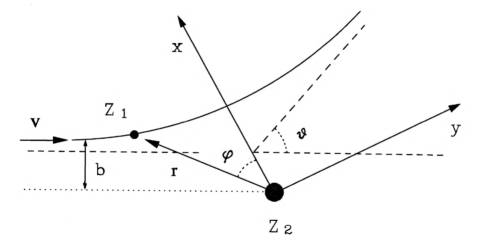
Figure 1: Coulomb excitation occurs when a charged projectile passes by a target nucleus along a Rutherford trajectory. The coordinates used in text are shown.

The simplest treatment that one can give to the problem is a semi-classical calculation, where the incident particle describes a well defined trajectory, which is a classic hyperbolic trajectory of Rutherford scattering (see figure 1). It has been proven that this treatment is valid in almost all situations studied in Coulomb excitation at low energies [AW75]. For high energy collisions, because the nuclear interaction distorts the scattering waves appreciably, a quantum treatment might be necessary for some observables, e.g. angular distributions [BN93]. Fortunately, at high energies, one can use the eikonal approximation for the scattering waves, which simplifies enormously the calculations.

The fundamental review paper [Ald56] contains a great deal of information on the subject and even now does not look obsolete, 40 years after its publication. However, in the last decades collisions between relativistic nuclei, with energies $E_{lab}>50$ MeV/nucleon, have become a main tool of investigation in nuclear physics, in particular for the study of nuclei far from the stability. Many new aspects of Coulomb excitation theory, such as the inclusion of transitions in/into the continuum, have been developed in the last two decades. It is thus timely to discuss the theory of Coulomb excitation from low to relativistic energies. These notes, far from being complete, reviews the main aspects of the theory of Coulomb excitation. As the reader will notice, very little is said about the nuclear interaction as I want to emphasize the role of the Coulomb interaction in the excitation process. Also, nuclear structure and nuclear excitation models are discussed only schematically and focused mainly on collective properties, such as the giant and pigmy resonances.

The readers are encouraged to study the Appendix section, where many basic quantum mechanics tools are discussed. These tools will be used throughout the text.

Beforehand, I would like to thank the JUSTIPEN (Japan-USA Theory Institute for Physics with Exotic Nuclei) for the financial support. Special thanks to Takaharu Otsuka, Takashi Nakatsukasa and Naoyuki Itagaki for the invitation to participate in this school and for hosting my visit to Japan.

II Interaction of photons with matter

II.1 Electrostatic multipoles

Electromagnetic multipoles appear in classical field theory as a result of the multipole expansion of the fields created by a finite system of charges and currents. We start with the system of point-like classical particles with electric charges $e_{i}$ located at the points $\mathbf{r}_{i}$.

The electrostatic potential of this system measured at the point $\mathbf{r}$ is given by the Coulomb law,

$$V(\mathbf{r})=\sum_{i}\frac{e_{i}}{|\mathbf{r}-\mathbf{r}_{i}|}.$$ (6)

The function

$$\frac{1}{|\mathbf{r}-\mathbf{r}^{\prime}|}=\frac{1}{\sqrt{r^{2}+r^{\prime 2}-2rr^{\prime}\cos\gamma}}$$ (7)

depends on the lengths $r,r^{\prime}$ of two vectors and the angle $\gamma$ between them rather than on the angles of the vectors $\mathbf{r}$ and $\mathbf{r}^{\prime}$ separately. If $\mathbf{r}\neq\mathbf{r}^{\prime}$, this function has no singularities and can be expressed with the aid of the expansion over the infinite set of Legendre polynomials with the coefficients depending on $r$ and $r^{\prime}$,

$$\frac{1}{|\mathbf{r}-\mathbf{r}^{\prime}|}=\sum_{L=0}^{\infty}P_{L}(\cos\gamma)f_{L}(r,r^{\prime}).$$ (8)

Using the notations $r_{<}$ and $r_{>}$ for the smaller and the greater $r$ and $r^{\prime}$, one can show that the expansion (8) takes the form

$$\frac{1}{|\mathbf{r}-\mathbf{r}^{\prime}|}=\sum_{L}\frac{r_{<}^{L}}{r_{>}^{L+1}}P_{L}(\cos\gamma).$$ (9)

The applications of the multipole expansion usually consider the potential (6) outside the system, i.e. at the point $\mathbf{r}$ with $r>r_{i}$. Then we can use the expansion (9) and the addition theorem

$$P_{L}(\cos\gamma)=\frac{4\pi}{2L+1}\sum_{M}Y_{LM}(\mathbf{n})Y^{\ast}_{LM}(\mathbf{n^{\prime}}),$$ (10)

where $\mathbf{n}$ ($\mathbf{n^{\prime}}$) is the direction of ${\bf r}$ (${\bf r^{\prime}}$). With that we get

$$V(\mathbf{r})=\sum_{LM}\frac{4\pi}{2L+1}\frac{1}{r^{L+1}}Y_{LM}^{\ast}(\mathbf{n})\mathcal{M}(EL,M).$$ (11)

Here the electric multipole moment of rank $L,\;L=0,1,...$, is defined for a system of point-like charges $i=1,2,...,A$ as a set of $(2L+1)$ quantities

$$\mathcal{M}(EL,M)=\sum_{i}e_{i}r_{i}^{L}Y_{LM}(\mathbf{n}_{i}),\quad M=-L,-L+1,...,+L,$$ (12)

where the sum runs over all charges $e_{i}$ located at $\mathbf{r}_{i}=(r_{i},\theta_{i},\varphi_{i})\equiv(r_{i},\mathbf{n}_{i})$. Exactly in the same way one can define, instead of the charge distribution, multipole moments for any other property of the particles, for example for the mass distribution, $e_{i}\rightarrow\rho_{i}$.

In quantum theory, multipole moments are to be considered as operators acting on the variables of the particles. Containing explicitly the spherical functions, the operator $\mathcal{M}(EL,M)$ has the necessary features of the tensor operator of rank $L$. Introducing the charge density operator

$$\rho(\mathbf{r})=\sum_{i}e_{i}\delta(\mathbf{r}-\mathbf{r}_{i}),$$ (13)

we come to a more general form of the multipole moment,

$$\mathcal{M}(EL,M)=\int d^{3}r\,\rho(\mathbf{r})r^{L}Y_{LM}(\mathbf{n}),\quad\mathbf{n}=\frac{\mathbf{r}}{r}.$$ (14)

In this form we even do not need to make an assumption of existence of point-like constituents in the system; for example, in the nucleus charged pions and other mediators of nuclear forces are included here along with the nucleons if $\rho(\mathbf{r})$ is the total operator of electric charge density. As expected, we can separate the geometry of multipole operators from their dynamical origin.

The lowest multipole moment $L=0$ is the monopole one. It determines the scalar part, the total electric charge $Ze$,

$$\mathcal{M}(E0,0)=\frac{1}{\sqrt{4\pi}}\sum_{i}e_{i}=\frac{1}{\sqrt{4\pi}}\int d^{3}r\,\rho(\mathbf{r})=\frac{1}{\sqrt{4\pi}}Ze.$$ (15)

The next term, $L=1$, defines the vector of the dipole moment

$$\mathbf{d}=\sum_{i}e_{i}\mathbf{r}_{i}=\int d^{3}r\,\rho(\mathbf{r})\mathbf{r}.$$ (16)

Taking into account the relation between the vectors and the spherical functions of rank $L=1$, we obtain

$$\mathcal{M}(E1,M)=\sqrt{\frac{3}{4\pi}}\sum_{i}e_{i}r_{i}(n_{i})_{M}=\sqrt{\frac{3}{4\pi}}d_{M}.$$ (17)

Subsequent terms of the multipole expansion determine the quadrupole ($L=2$), octupole ($L=3$), hexadecapole ($L=4$), and higher moments.

In a similar way one can define magnetic multipoles $\mathcal{M}(ML,M)$ related to the distribution of currents. The convection current due to orbital motion and the magnetization current generated by the spin magnetic moments determine corresponding contributions to the magnetic multipole moment of rank $L$,

$$\mathcal{M}(ML,M)=\sum_{i}\Bigl{(}g_{i}^{s}\mathbf{s}_{i}+\frac{2}{L+1}g_{i}^{L}\mathbf{l}_{i}\Bigr{)}\cdot\mbox{\boldmath$\nabla$}\Bigl{(}r_{i}^{L}Y_{LM}(\mathbf{n}_{i})\Bigr{)}.$$ (18)

Here $\mathbf{s}_{i}$ and $\mathbf{l}_{i}$ stand for the spin and orbital angular momentum of a particle $i$, respectively; $g_{i}^{s}$ and $g_{i}^{L}$ are corresponding gyromagnetic ratios. (In this section, we measure all angular momenta in units of $\hbar$ and the gyromagnetic ratios in the magnetons $e\hbar/(2m_{i}c)$).

The expression (18) vanishes for $L=0$ demonstrating the absence of magnetic monopoles. At $L=1$, we come to the spherical components $\mu_{M}$ of the magnetic moment $\mu$,

$$\mathcal{M}(M1,M)=\sqrt{\frac{3}{4\pi}}\mu_{M},$$ (19)

$$\mbox{\boldmath$\mu$}=\sum_{i}(g_{i}^{s}\mathbf{s}_{i}+g_{i}^{L}\mathbf{l}_{i}).$$ (20)

Higher terms determine magnetic quadrupole, $L=2$, magnetic octupole, $L=3$, and so on.

II.2 Real photons

II.2.1 Radiative decay

The probability for the radiative (by emission of a photon) transition for a nuclear transition $i\rightarrow f$ integrated over angles of the emitted photon and summed over its polarizations involves the same electromagnetic matrix elements as discussed above. We will not derive the equations but only quote the results for the the probability for radiative decay [Ald56]:

$$w_{fi}=\frac{8\pi(L+1)}{L[(2L+1)!!]^{2}\hbar}\kappa^{2L+1}$$

$$\times \sum_{LM}\Bigl{\{}\Bigl{|}\Bigl{(}{\cal M}({\rm EL},M)\Bigr{)}_{fi}\Bigr{|}^{2}+\Bigl{|}\Bigl{(}{\cal M}({\rm ML},M)\Bigr{)}_{fi}\Bigr{|}^{2}\Bigr{\}}$$

where $\kappa=\omega/c$, and the multipole matrix elements for electric and magnetic transitions are expressed via the current operator ${\bf j}({\bf r})$,

$${\cal M}({\rm ML},M)=\int d^{3}r({\bf j}\cdot\hat{{\bf l}})\Phi_{LM},$$ (22)

$${\cal M}({\rm EL},M)=\int d^{3}r\Bigl{[}(\mbox{\boldmath$\nabla$}\cdot{\bf j})\frac{1}{\kappa}\frac{\partial}{\partial r}r-\kappa({\bf r}\cdot{\bf j})\Bigr{]}\Phi_{LM},$$ (23)

${\bf l}=-i[{\bf r}\times\mbox{\boldmath$\nabla$}]$ is the orbital momentum operator and the function $\Phi_{LM}$ arises from the partial wave expansion of the plane wave,

$$\Phi_{LM}=-i\frac{(2L+1)!!}{L+1}\frac{1}{c\kappa^{L}}j_{L}(\kappa r)Y_{LM}({\bf n}),$$ (24)

where $j_{L}(\kappa r)$ are spherical Bessel functions. Of course, for a given pair of states $f,i$ and a given multipolarity $L$, only one term, either electric or magnetic, in (LABEL:81) works if parity is conserved.

An important practical case is connected to the long wavelength radiation: $\lambda\sim 1/\kappa\gg R$ where $R$ is a size of the system. In nuclei $R\approx 1.2\,A^{1/3}$ fm so that the condition

$$\kappa R\ll 1$$ (25)

is equivalent to $\hbar\omega\ll 165A^{-1/3}$ MeV which is usually fulfilled. In the long wavelength approximation, we can use the limiting values of spherical Bessel functions $j_{L}(x)\approx x^{L}/(2L+1)!!$ at small arguments $x$. Then the magnetic multipoles (22) become

$${\cal M}({\rm ML},M)=-\frac{i}{c(L+1)}\int d^{3}r\Bigl{(}{\bf j}({\bf r})\cdot\hat{{\bf l}}\Bigr{)}r^{L}Y_{LM}({\bf n})$$ (26)

One can show that for the orbital current in Eq. (18), this expression coincides with the orbital part of the static magnetic moment [EG88]. The presence of spin implies magnetization currents. In macroscopic electrodynamics such a current is $c[\mbox{\boldmath$\nabla$}\times{\bf m}]$ where ${\bf m}$ stands for the magnetization density. The analogous quantity for a quantum particle is

$${\bf m}({\bf r})=\sum_{a}g^{s}_{a}{\bf s}_{a}\delta({\bf r}-{\bf r}_{a}).$$ (27)

The induced spin current is

$${\bf j}_{{\rm spin}}=c\sum_{a}g_{a}^{s}[\mbox{\boldmath$\nabla$}\times{\bf s}_{a}]\delta({\bf r}-{\bf r}_{a}).$$ (28)

Being substituted into (26), this current reproduces the spin part of static magnetic multipoles as in (18).

In the long wavelength limit, the second term of the electric multipole (23) is smaller by a factor $(kR)^{2}$ than the first one. In the first term $\bm{\nabla}\cdot{\bf j}$ reduces to the time derivative of the charge density $\rho^{ch}$ with the aid of the continuity equation,

$$\bm{\nabla}\cdot{\bf j}+\partial\rho^{ch}/\partial t=0.$$ (29)

This time derivative can be expressed through the difference of energies between the initial and final states gives $\hbar\omega_{{\bf k}}$. Performing the expansion of the spherical Bessel functions we come to

$${\cal M}({\rm EL},M)=\int d^{3}r\rho^{ch}({\bf r})r^{L}Y_{LM}({\bf n})$$ (30)

which is a standard definition of the electric multipoles.

Usually the angular momentum projection $M_{f}$ of the final state is not measured. Then we have to sum the transition rate over all $M_{f}$ defining the reduced transition probability

$$B({\rm EL};i\rightarrow f)=\sum_{MM_{f}}\Bigl{|}\Bigl{(}{\cal M}({\rm EL},M)\Bigr{)}_{fi}\Bigr{|}^{2}.$$ (31)

According to the Wigner-Eckart theorem [BM75], the entire dependence of the matrix element on the magnetic quantum numbers is concentrated in the Clebsch-Gordan coefficients of vector addition. Using instead the Wigner $3j$-symbols, we have for any tensor operator $T_{LM}$

$$\langle J_{f}M_{f}|T_{LM}|J_{i}M_{i}\rangle=$$

$$(-)^{J_{f}-M_{f}}\left(\begin{array}[]{ccc}J_{f}&L&J_{i}\\ -M_{f}&M&M_{i}\end{array}\right)\left<f\|T_{L}\|i\right>,$$ (34)

where the reduced matrix element $\left<f\|T_{L}\|i\right>$ does not depend on projections. We can use the orthogonality of the vector coupling coefficients and perform the summation over $M$ and $M_{f}$.

The reduced transition probability is then related to the reduced matrix element of the multipole operator,

$$B({\rm EL};i\rightarrow f)=\frac{1}{2J_{i}+1}\Bigl{|}(f\|{\cal M}\left<{\rm EL})\|i\right>\Bigr{|}^{2}.$$ (35)

This quantity is convenient because it does not depend on the initial population of various projections $M_{i}$. Note that for the inverse transition induced by the same operator, the detailed balance relation is valid,

$$B({\rm EL};f\rightarrow i)=\frac{2J_{i}+1}{2J_{f}+1}B({\rm EL};i\rightarrow f).$$ (36)

The reduced transition probability determines the partial lifetime of a given initial state with respect to a specific radiative decay (all $M_{f}$ summed up),

$$\tau^{-1}_{i\rightarrow f}=\sum_{M_{f}}w_{fi}=\frac{8\pi}{\hbar}\frac{L+1}{L[(2L+1)!!]^{2}}k^{2L+1}B({\rm EL};i\rightarrow f).$$ (37)

Here the kinematic factors are singled out. They are associated with the geometry and phase space volume of the emitted photon. Information concerning structure of the radiating system is accumulated in the reduced transition probability. With the substitution EL$\rightarrow$ML, the same expressions are valid for magnetic multipoles.

Classically, the electromagnetic radiation emitted by a system is the result of the variation in time of the charge density or of the distribution of charge currents in the system. The energy is emitted in two types of multipole radiation: the electric and the magnetic. Each one of them is expressed as function of the corresponding multipole moments, being the quantities which contain the variables (charge and current) of the system. If the wavelength of the emitted radiation is long in comparison to the dimensions of the system (which is valid for a $\gamma$-ray of $\lesssim\,10$ MeV energy) the power emitted by each multipole is given by ([Ja75], chap.16):

$$P_{E}(LM)={\frac{8\pi(L+1)c}{L[(2L+1)!!]^{2}}}\left({\frac{\omega}{c}}\right)^{2L+2}|{\cal M}(EL,M)|^{2}$$ (38)

for electric multipole radiation and

$$P_{M}(LM)={\frac{8\pi(L+1)c}{L[(2L+1)!!]^{2}}}\left({\frac{\omega}{c}}\right)^{2L+2}|{\cal M}(ML,M)|^{2}.$$ (39)

In quantum mechanics, the energy is not emitted continually but in packets of energy $\hbar\omega$. In a quantum calculation the disintegration constant is the same as the number of quanta emitted per unit of time when the power is given by the classical expressions (38) and (39). Thus,

$$\lambda_{E}(LM) = {\frac{P_{E}(LM)}{\hbar\omega}}$$

$$= {\frac{8\pi(L+1)}{\hbar L[(2L+1)!!]^{2}}}\left({\frac{\omega}{c}}\right)^{2L+1}|{\cal M}(EL;M)|^{2}$$

and

$$\lambda_{M}(LM) = {\frac{P_{M}(LM)}{\hbar\omega}}$$

$$= {\frac{8\pi(L+1)}{\hbar L[(2L+1)!!]^{2}}}\left({\frac{\omega}{c}}\right)^{2L+1}|{\cal M}(M,LM)|^{2}.$$

The decaying nucleus should also be treated as a quantum system. In this sense, the expressions for the multipole moments ${\cal M}(EL,M)$ and ${\cal M}(ML,M)$ continue to have validity if we use for the charge and current densities the quantum expressions

$$\rho_{fi}(\mathbf{r})=\Psi_{f}^{\ast}(\mathbf{r})\Psi_{i}(\mathbf{r}),$$ (42)

$$\mathbf{j}_{fi}(\mathbf{r})={\frac{e\hbar}{2im}}\left[\Psi_{f}^{\ast}(\mathbf{\mbox{\boldmath$\nabla$}}\Psi_{i})-(\mathbf{\mbox{\boldmath$\nabla$}}\Psi_{f}^{\ast})\Psi_{i}\right],$$ (43)

where the argument $i$ ($f$) denotes the initial (final) state described by the wavefunction $\Psi_{i}\ (\Psi_{f}).$ Equations (42) and (43) refer to a single nucleon with mass $m$ that emits radiation in its passage from the state $i$ to the state $f$. Thus, a sum over all the protons should be incorporated to the result, when we do the substitution of eqs. (42) and (43) in eqs. (LABEL:8.7) and (LABEL:8.8) ([Ja75], chap. 16).

Not only are the values of the magnetic multipole moments are small in comparison to the electric moments of same order, but also the transition probability decreases quickly with increasing $L$, restricting the multipole orders that give significant contribution. To show this, it is sufficient to observe that the product $(\omega/c)^{L}{\cal M}(EL,M)$ in (LABEL:8.7) is at most equal to $Ze(\omega R/c)^{L}$, where $R$ is the radius of the nucleus. For the energy that we consider, $\omega R/c$ is very small implying that, for the larger powers of $L$, the disintegration constant is also very small. These facts imply, in principle, that the electric dipole is always the dominant radiation. But the selection rules that we will see next can modify this situation.

II.2.2 Selection Rules

The conservation of angular momentum and parity can prohibit certain $\gamma$ transitions between two states. The selection rules for the $\gamma$-radiation are easy to establish if we accept the fact that a quantum of radiation carries an angular momentum L of module $\sqrt{L(L+1)}\,\hbar$ and component $z$ equal to $M\hbar$, where $L$ is the multipolar order. Thus, in transition between an initial spin $\mathbf{I}_{i}$ and a final spin $\mathbf{I}_{f}$ the conservation of angular momentum imposes $\mathbf{I}_{i}=\mathbf{I}_{f}+\mathbf{L}$ and, in this way, the possible values for the multipole order $L$ should obey

$$|I_{i}-I_{f}|\leq l\leq I_{i}+I_{f},$$ (44)

where $|\mathbf{I}_{i}|=\sqrt{I_{i}(I_{i}+1)}\,\hbar$, etc. A special case is the transition $0^{+}\rightarrow 0^{+}$: as multipole radiation of order zero, these transitions do not exist and they are effectively impossible through the emission of a $\gamma$-ray. But in this case a process of internal conversion can happen, where the energy is released by the ejection of an atomic electron.

Transitions between states of same parity can only be accomplished by electric multipole radiation of even number or by magnetic radiation of odd number. The inverse is valid for transitions where there is parity change. Why this happens can be understood examining the definitions of the multipole moments. The functions that compose the integrand have definite parity and it is necessary that the integrand has even parity, otherwise the contribution in r cancels with the contribution in $-$r and the integral over the whole space vanishes. Let us look at the case of Eq. (30): $r^{L}$ is always positive and the spherical harmonic $Y_{L}^{M}(\theta,\phi)$ is even if $L$ is even. For Eq. (30) to be non-zero, $\Psi_{i}$ should have the same parity of $\Psi_{f}$ for $L$ even and opposite parity for $L$ odd. This justifies the transition rule for the electric multipole radiation. A similar procedure applied to Eq. (26) justifies the selection rules for the magnetic multipole radiation.

Let us take an example: if the initial state is a $3^{+}$ and the final a $2^{-}$, the possible values of $L$ will be 1, 2, 3, 4 and 5. But the change of parity restricts the transitions to E1, M2, E3, M4 and E5, where E1 symbolizes an electric dipole transition ($L=1$), etc.

II.2.3 Estimate of the Disintegration Constants

The use of Eq. (LABEL:8.7) and (LABEL:8.8) for the calculation of the transition probabilities in a real nucleus has the difficulty that wavefunctions that appear in eqs. (42) and (43) are not known. But, a prediction of their order of magnitude for the several modes can be done by assuming a single proton decaying from an excited state described by the wavefunction $\Psi_{i}$ to a final state $f$ with $L=0$. as shown in figure 2.

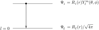
Figure 2: De-excitation of a proton to a level with $L=0$.

For an approximate calculation it is enough to do:

$$R_{i}(r) =\text{const.}=R_{i}\qquad(r<R),$$

$$R_{i}(r) =0\qquad(r>R)$$ (45)

and to use the same approach for $R_{f}(r)$. The normalization yields immediately the values for the constants $R_{i}$ and $R_{f}$:

$$R_{i}=R_{f}=\sqrt{\frac{3}{R^{3}}},$$ (46)

where $R$ is the nuclear radius. In this way, it is not difficult to calculate the electric multipole moment ${\cal M}(EL,M)$:

$${\cal M}(EL,M)=e\int r^{L}Y_{L}^{M\ast}(\theta,\phi){\frac{3}{R^{3}}}{\frac{Y_{L}^{M}(\theta,\phi)}{\sqrt{4\pi}}}r^{2}\,dr\,d\Omega,$$ (47)

which yields

$${\cal M}(EL,M)={\frac{3eR^{L}}{\sqrt{4\pi}(L+3)}}.$$ (48)

Thus, in this approximation, the disintegration constant in Eq. (LABEL:8.7) is

$$\lambda_{E}={\frac{2(L+1)}{L[(2L+1)!!]^{2}}}\left({\frac{3}{L+3}}\right)^{2}{\frac{e^{2}}{\hbar}}\left({\frac{E_{\gamma}}{\hbar c}}\right)^{2L+1}R^{2L},$$ (49)

where we wrote explicitly the disintegration energy $E_{\gamma}=\hbar\omega$. A similar calculation for the magnetic disintegration constant in Eq. (LABEL:8.8) yields

$$\lambda_{M} = {\frac{20(L+1)}{L[(2L+1)!!]^{2}}}\left({\frac{3}{L+3}}\right)^{2}{\frac{e^{2}}{\hbar}}\left({\frac{E_{\gamma}}{\hbar c}}\right)^{2L+1}$$ (50)

$$\times R^{2L}\left({\frac{\hbar}{mcR}}\right)^{2},$$

where $m$ is the mass of a nucleon. For a typical nucleus of intermediate mass of $A=120$, it is easy to see that $\lambda_{E}/\lambda_{M}\cong 100$, independently of the multipolar order $L$. Evidently, both constants decrease rapidly when the value of $L$ increases.

Figure 3: Distribution of the ratio between the experimental and theoretical disintegration constants for transitions of the E1 and E2 type [Sk66].

Disagreements of several orders of magnitude between the result of the calculation above and the corresponding experimental values can happen. In particular, if the experimental disintegration rates are smaller than the ones predicted by eqs. (49) and (50), that can mean that Eq. (45) is not very reasonable and that the small interception of the wavefunctions $\Psi_{i}$ and $\Psi_{f}$ decrease the values of $\lambda$. Experimental values higher than predicted by eqs. (49) and (50) can mean, on the other hand, that the transition involves the participation of more than one nucleon or even a collective participation of the whole nucleus.

Figures 3 and 4 illustrate the two situations: in figure 3 the experimental values of $\lambda$ for transitions of E1 multipolarity are orders of magnitude smaller than that calculated from Eq. (49). The opposite happens with the E2 multipolarity where in most cases the experimental rate is larger than calculated; this is due to the fact that E2 transitions are common among levels of collective bands, especially rotational bands in deformed nuclei. In figure 4, on the other hand, what one notices is very good agreement between theoretical values and experimental ones for M4. This behavior is typical of transitions of high multipolarity.

III Low energy collisions

Coulomb excitation involves the same nuclear matrix elements as in radiative decay, but with different phase space factors. The reason is that Coulomb excitation is a process in which the excitation occurs when nuclei are outside their mutual charge distributions. Therefore, the Maxwell equation $\bm{\nabla}\cdot{\bf E}=0$ applies for the electric field inducing the transition. This means that only transverse photons fields, the same as for real photons, appear in Coulomb excitation [EG88]. In this section, we will prove this statement, and we will describe the semiclassical theory of Coulomb excitation for low energy collisions.

III.1 Central collisions

According to Eq. (390) of the Appendix C, the probability of exciting the nucleus to a state $f$ above the ground state $i$ is

$$a_{if}=-{\frac{i}{\hbar}}\int V_{if}\,e^{i\omega t}\,dt,$$ (51)

with $\omega=(E_{f}-E_{i})/\hbar$, is the probability amplitude that there will be a transition $i\rightarrow f$. The matrix element

$$V_{if}=\int\Psi_{f}^{\ast}V\Psi_{i}\,d\tau$$ (52)

contains a potential $V$ of interaction of the incident particle with the nucleus. The square of $a_{if}$ measures the transition probability from $i$ to $f$ and this probability should be integrated along the trajectory.

A simple calculation can be done in the case of the excitation of the ground state $J=0$ of a deformed nucleus to an excited state with $J=2$ as a result of a frontal collision with scattering angle of $\theta=180^{\circ}$. The perturbation $V$ comes, in this case, from the interaction of the charge $Z_{p}e$ of the projectile with the quadrupole moment of the target nucleus. This quadrupole moment should work as an operator that acts between the initial and final states. The way of adapting (11) is writing

$$V={\frac{1}{2}}{\frac{Z_{p}e^{2}Q_{if}}{r^{3}}},$$ (53)

with

$$Q_{if}=\sum_{i}\int\Psi_{f}^{\ast}(3z_{i}^{2}-r_{i}^{2})\Psi_{i}\,d\tau,$$ (54)

where the sum extends to all protons. The excitation amplitude is then written as

$$a_{if}={\frac{Z_{p}e^{2}Q_{if}}{2i\hbar}}\int{\frac{e^{i\omega t}}{r^{3}}}\,dt.$$ (55)

Figure 4: $\tau_{(half-life)}>R^{6}$ (R= nuclear radius, $c=1$) as a function of the energy of the $\gamma$-ray for a series of transitions of the M4 type. One sees  good agreement between the theoretical estimate (straight line) and the experimental data [GS51].

At an scattering of $\theta=180^{\circ}$ a relationship exists between the separation $r$, the velocity $v$, the initial velocity $v_{0}$ and the distance of closest approach $a=2a_{0}$:

$$v={\frac{dr}{dt}}=\pm v_{0}\left(1-{\frac{a}{r}}\right)^{1/2},$$ (56)

which is obtained easily from the conservation of energy. Besides, if the excitation energy is small, we can assume that the factor $e^{i\omega t}$ in (55) does not vary much during the time that the projectile is close to the nucleus. Thus, this factor can be placed outside the integral and it does not contribute to the cross section. One gets

$$a_{if}={\frac{Z_{p}e^{2}Q_{if}}{2i\hbar v_{0}}}\times 2\int{\frac{dr}{r^{3}(1-a/r)^{1/2}}}.$$ (57)

The integral is solved easily by the substitution $u=1-a/r$, in what results

$$a_{if}={\frac{4Z_{p}e^{2}Q_{if}}{3i\hbar v_{0}a^{2}}}={\frac{4Q_{if}E^{2}}{3Z_{p}e^{2}\hbar v_{0}Z_{T}^{2}}},$$ (58)

where the conservation of energy, $E={\frac{1}{2}}m_{0}v_{0}^{2}=Z_{p}Z_{T}e^{2}/a$ was used, with $m_{0}$ being the reduced mass of the projectile+target system and $Z_{T}$ the atomic number of the target. The differential cross section is given by the product of the Rutherford differential cross section at 180^∘ and the excitation probability along the trajectory, measured by the square of $a_{if}$:

$$\left.{\frac{d\sigma}{d\Omega}}\right|_{\theta=180^{\circ}}={\frac{d\sigma_{R}}{d\Omega}}\left|{}_{\theta=180^{\circ}}\right.\times|a_{if}|^{2}.$$ (59)

The Rutherford differential cross section is the classic expression

$${\frac{d\sigma_{R}}{d\Omega}}=\left({\frac{Z_{p}Z_{T}e^{2}}{4E}}\right)^{2}\sin^{-4}\left({\frac{\theta}{2}}\right)$$ (60)

and, at $\theta=180^{\circ}$, we obtain

$$\left.{\frac{d\sigma}{d\Omega}}\right|_{\theta=180^{\circ}}={\frac{m_{0}E|Q_{if}|^{2}}{18\hbar^{2}Z_{T}^{2}}},$$ (61)

an expression that is independent of the charge of the projectile. It is, on the other hand, proportional to the mass of the projectile, indicating that heavy ions are more effective for Coulomb excitation.

The quadrupole moment operator $Q_{if}$ uses, as we saw, the wavefunctions $\Psi_{i}$ and $\Psi_{f}$ of the initial and final states. If those two wavefunctions are similar, as is the case of an excitation to the first level of a rotational band, the operator $Q_{if}$ can be replaced by the intrinsic quadrupole moment $Q$. The expression (61) translates, in this way, the possibility to evaluate the quadrupole moment from a measurement of a value of the cross section.

III.2 Electric excitations

The interaction hamiltonian responsible for the excitation processes in the nonrelativistic case can be written as

$$H^{\prime}=\int d^{3}r_{1}d^{3}r_{2}\frac{\rho^{ch}_{1}({\bf r}_{1}-{\bf R}_{1})\rho^{ch}_{2}({\bf r}_{2}-{\bf R}_{2})}{|{\bf r}_{1}-{\bf r}_{2}|}-\frac{Z_{1}Z_{2}e^{2}}{R(t)}$$ (62)

where charge densities of unperturbed nuclei depend on the distances from the corresponding centers. We subtracted the interaction between nuclei as a whole which determines the trajectory (time dependence of ${\bf R}={\bf R}_{1}-{\bf R}_{2}$) but does not contribute to intrinsic excitations. We introduce the intrinsic coordinates for each nucleus ${\bf x}_{1,2}={\bf r}_{1,2}-{\bf R}_{1,2}$,

$$H^{\prime}=\int d^{3}x_{1}d^{3}x_{2}\frac{\rho_{1}^{ch}({\bf x}_{1})\rho_{2}^{ch}({\bf x}_{2})}{|{\bf R}(t)+{\bf x}_{1}-{\bf x}_{2}|}-\frac{Z_{1}Z_{2}e^{2}}{R(t)},$$ (63)

and carry out the multipole expansion for a large distance between the centers, $R\gg x_{1,2}$,

$$H^{\prime} = \int d^{3}x_{1}d^{3}x_{2}\rho_{1}^{ch}({\bf x}_{1})\rho_{2}^{ch}({\bf x}_{2})$$ (64)

$$\times \sum_{L>0,M}\frac{4\pi}{2L+1}\frac{x_{12}^{L}}{R^{L+1}(t)}Y_{LM}({\bf x}_{12})Y_{LM}^{\ast}({\bf R}).$$

Here ${\bf x}_{12}\equiv{\bf x}_{1}-{\bf x}_{2}$.

This hamiltonian is rather complicated due to the correlations associated with the mutual excitation of the nuclei. It becomes much simpler if we are interested in the excitation of one of the partners only. Let the “projectile” 2 be not excited and we can neglect effects related to its structure as an extended object. Then $\rho^{ch}_{2}({\bf x}_{2})\approx Z_{2}e\delta({\bf x}_{2})$, and the hamiltonian is expressed in terms of the electric multipole moments of the “target” 1,

$$H^{\prime}=Z_{2}e\sum_{L>0,M}\frac{4\pi}{2L+1}\frac{1}{R^{L+1}(t)}Y^{\ast}_{LM}({\bf R}(t)){\cal M}({\rm EL},M).$$ (65)

The hamiltonian (65) is time-dependent since the trajectory is considered as a given function of time. According to Eq. (390) the transition amplitude $i\rightarrow f$ with excitation by $\hbar\omega=E_{f}-E_{i}$ is the Fourier component for the transition frequency of the interaction hamiltonian taken along the unperturbed trajectory,

$$a_{fi}=-\frac{i}{\hbar}\int_{-\infty}^{\infty}dtH_{fi}^{\prime}(t)e^{i\omega t}.$$ (66)

For the unpolarized initial nuclei and with no final polarization registered, the transition rate is to be averaged over initial projections and summed over final projections of the target,

$$w_{fi}=\frac{1}{2J_{i}+1}\sum_{M_{f}M_{i}}|a_{fi}|^{2};$$ (67)

the polarization state of the projectile is assumed to be unchanged.

The trajectory enters the result via the time integral

$$I_{LM}(\omega)=\int_{-\infty}^{\infty}dt\frac{1}{R^{L+1}(t)}Y_{LM}({\bf R}(t))e^{i\omega t}.$$ (68)

This Fourier component becomes small, $\propto\exp(-{\rm const}\cdot\zeta)$, if the trajectory changes at too slowly a rate compared to the needed transition frequency and the parameter of adiabaticity $\zeta>1$. We will discuss more about this integral later.

The intrinsic matrix elements of multipole moments appear in the transition rate (67) in sums over magnetic quantum numbers

$$\Sigma_{LM,L^{\prime}M^{\prime}}=\frac{1}{2J_{i}+1}\sum_{M_{f}M_{i}}{\cal M}_{fi}({\rm EL},M){\cal M}_{fi}^{\ast}({\rm EL^{\prime}},M^{\prime}).$$ (69)

The summation in Eq. (69) selects $L^{\prime}=L,M^{\prime}=M$ and the result does not depend on $M$.

$$\Sigma_{LM,L^{\prime}M^{\prime}} = \frac{1}{2J_{i}+1}\sum_{M_{f}M_{i}}\Bigl{|}{\cal M}_{fi}({\rm EL},M)\Bigr{|}^{2}\delta_{LL^{\prime}}\delta_{MM^{\prime}}$$ (70)

$$= \frac{B({\rm EL};i\rightarrow f)}{2L+1}\delta_{LL^{\prime}}\delta_{MM^{\prime}},$$

where $B({\rm EL};i\rightarrow f)$ are given by Eq. (35).

The total excitation probability is therefore

$$w_{fi}=\Bigl{(}\frac{4\pi Z_{2}e}{\hbar}\Bigr{)}^{2}\sum_{L>0}\frac{B({\rm EL};i\rightarrow f)}{(2L+1)^{3}}\sum_{M}|I_{LM}(\omega_{fi})|^{2}.$$ (71)

From the viewpoint of the projectile the process is inelastic scattering. The Coulomb trajectory defines the deflection angle $\theta$ and the Rutherford cross section, Eq. (60). In our approximation, the trajectory is not influenced by the target excitation so that the inelastic cross section is factorized into the product of the Rutherford cross section (60) and the excitation probability (71),

$$d\sigma_{fi}=d\sigma_{R}w_{fi}=\sum_{L>0}d\sigma_{fi}({\rm EL})$$ (72)

where the cross section for the excitation of multipolarity $L$ is equal to

$$\frac{d\sigma_{fi}({\rm L})}{d\Omega}=\Bigl{(}\frac{\pi Z_{2}ea}{\hbar\sin^{2}(\theta/2)}\Bigr{)}^{2}\frac{B({\rm EL};i\rightarrow f)}{(2L+1)^{3}}\sum_{M}|I_{LM}(\omega_{fi})|^{2},$$ (73)

where $a$ is the distance of closest approach, Eq. (2).

This theory can be extended, considering quantum scattering instead of classical trajectories, using relativistic kinematics, taking into account magnetic multipoles which become equally important for relativistic velocities, and including higher order processes of sequential excitation of nuclear states. The last generalization is necessary for excitation of rotational bands and overtones of giant resonances (quantum states with several vibrational quanta). The mutual excitation of the projectile and of the target can also be studied.

III.3 Estimates

We can make a crude estimate of the cross section of Coulomb excitation. The trajectory integral (68), after changing the variable to $dR=vdt$, gives the dimensional factor $a^{-L}/v$. It has to be taken near the closest approach point (2) which is the most effective for excitation. The constants from the Rutherford cross section can be combined into the Coulomb parameter (1). As a result,

$$\sigma({\rm EL})\simeq\eta^{2}\frac{B({\rm EL})}{a^{2L-2}}f_{L}(\zeta)$$ (74)

where the function $f_{L}(\zeta)$ depends smoothly on $L$ but contains the exponential cut-off at large values of the adiabaticity parameter $\zeta$. We remember, Eq. (49), that in photoabsorption each consecutive multipole was suppressed by a factor $(kR)^{2}$. The situation for exciting higher multipoles is easier in the Coulomb excitation because here

$$\frac{\sigma({\rm E,L+1})}{\sigma({\rm EL})}\sim\frac{B({\rm E,L+1})}{B({\rm EL})a^{2}}\sim\Bigl{(}\frac{R}{a}\Bigl{)}^{2}.$$ (75)

This ratio is significantly larger than $(kR)^{2}$.

III.4 Inclusion of magnetic interactions

A more accurate description of Coulomb excitation for all scattering angles requires the correct treatment of magnetic interactions and the Coulomb recoil of the classical trajectories. Here we will discuss the role of magnetic interactions. Note that magnetic interactions induce electric transitions, too. And electric interactions also induce magnetic transitions. Thus, in electromagnetic excitation, both interactions mix and can only be isolated under special circumstances. We now show how magnetic interactions modify the results obtained in the last section.

Following the derivation of the electromagnetic interaction presented above, the excitation a target nucleus from an initial rate $\mid i>$ to a final state $\mid f>$ is, to first order, given by

$$a_{fi}=\frac{1}{i\hbar}\int_{-\infty}^{\infty}dt\;e^{i(E_{f}-E_{i})t/\hbar}<\;f\mid\mathcal{H}_{int}\mid i>$$ (76)

where (see Appendix D)

$$<f\mid\mathcal{H}_{int}\mid i>\;=\int\;\left[\rho_{fi}\phi(\mathbf{r},t)-\frac{1}{c}\;\mathbf{j}_{fi}(\mathbf{r})\cdot\mathbf{A}(\mathbf{r},t)\right]d^{3}r$$ (77)

with $\rho_{fi}({\bf r})$ and ${\bf j}_{fi}({\bf r})$ given by Eqs. (42) and (43), respectively.

Thus,

$$a_{fi}=\frac{1}{i\hbar}\int_{-\infty}^{\infty}dt\;e^{i\omega t}\left[\rho_{fi}(\mathbf{r})-\frac{\mathbf{v}\left(t\right)}{c^{2}}\cdot\mathbf{j}_{fi}(\mathbf{r})\right]\phi\left(\mathbf{r},t\right)d^{3}r.$$ (78)

where v is the velocity of the projectile, and we used

$$\mathbf{A}(\mathbf{r},t)=\dfrac{\mathbf{v}\left(t\right)}{c}\phi\left(\mathbf{r},t\right),$$ (79)

valid for a spinless projectile following a classical trajectory.

The scalar and vector potentials at the target nucleus interior,

$$\phi(\omega,\,\mathbf{r}) =Z_{p}e\int_{-\infty}^{\infty}e^{i\omega t}\,{\frac{1}{\mid\mathbf{r-r^{\prime}}(t)\mid}}\,dt$$ (80)

$$\mathbf{A}(\omega,\,\mathbf{r}) ={\frac{Z_{p}e}{c}}\int_{-\infty}^{\infty}\mathbf{v^{\prime}}(t)\,e^{i\omega t}\,{\frac{1}{\mid\mathbf{r-r^{\prime}}(t)\mid}}\,dt$$ (81)

are generated by a projectile with charge Z_p following a Coulomb trajectory, described by its time-dependent position $\mathbf{r}(t)$.

We now use the expansions of Eqs. (9) and (10) and, assuming that the projectile does not penetrate the target, we use $\mathbf{r}_{>}$ ($\mathbf{r}_{<}$) for the projectile (target) coordinates.

To perform the time-integrals, we need the time dependence, ${\bf r}^{\prime}(t)$, for a particle moving along the Rutherford trajectory, which can be directly obtained by solving the equation of angular momentum conservation (see [Go02]) for a given scattering angle $\vartheta$ in the center of mass system (see figure 1). Introducing the parametrization

$$r(\chi)={a_{0}}\,\left[\epsilon\,\cosh\chi+1\right]$$ (82)

where

$$a_{0}={\frac{Z_{p}Z_{T}e^{2}}{m_{0}v^{2}}=}\frac{a}{2}{,\ \ \ \ \ \ \ }\text{{and}}{\ \ \ \ \ }\epsilon={1\over\sin\left(\vartheta/2\right)}$$ (83)

one obtains [Go02]

$$t={\frac{a_{0}}{v}}\,\left[\chi+\epsilon\,\sinh\chi\right]\,.$$ (84)

Using the scattering plane perpendicular to the z-axis, one finds that the corresponding components of $\mathbf{r}$ may be written as

$$x =a_{0}\,\left[\cosh\chi+\epsilon\right],$$

$$y =a_{0}\,\sqrt{\epsilon^{2}-1}\,\sinh\chi,$$

$$z =0\ .$$ (85)

The impact parameter $b$ in figure 1 is related to the scattering angle ${\vartheta}$ by

$$b=a_{0}\cot\left({\vartheta/2}\right),$$ (86)

and the eccentricity parameter $\epsilon$ is related to it by means of

$$\epsilon=\sqrt{1+{b^{2}\over a_{0}^{2}}},$$ (87)

In the limit of straight-line motion $\epsilon\simeq b/a_{0}\gg 1$, and the equations above reduce to the simple straight-line parametrization,

$$y=vt\ ,\ \ \ \ \ \ \ x=b\ ,\ \ \ \mathrm{and}\ \ \ z=0\ .$$ (88)

Using the continuity equation, $\mathbf{\nabla}\cdot\mathbf{j}_{fi}=-i\omega\rho_{fi}$, for the nuclear transition current, the terms in the expansion of the scalar and vector potentials mix up. After a long but straightforward calculation, one can show that the result can be expressed in terms of spherical tensors (see, e.g., Ref. [EG88], Vol. II) and Eq. (78) becomes

$$a_{fi} = {\frac{Z_{p}e}{i\hbar}}\sum_{LM}\,{\frac{4\pi}{2L+1}}\,(-1)^{M}$$ (89)

$$\times \Big{[}S(EL,\,M)\mathbf{\mathcal{M}}_{fi}(EL,\,-M)$$

$$+ S(ML,\,M)\mathbf{\mathcal{M}}_{fi}(ML,\,-M)\Big{]}$$

where

$$\mathcal{M}_{fi}(EL,M) = {\frac{(2L+1)!!}{\kappa^{L+1}c(L+1)}}$$

$$\times \int\mathbf{j}_{fi}(\mathbf{r})\cdot\bm{\nabla}\times\mathbf{L}\left[j_{L}(\kappa r)Y_{LM}(\hat{\mathbf{r}})\right]d^{3}r\ ,$$

$$\mathcal{M}_{fi}(ML,M) = -i{\frac{(2L+1)!!}{\kappa^{L}c(L+1)}}$$ (91)

$$\times \int\mathbf{j}_{fi}(\mathbf{r})\cdot\mathbf{L}\left[j_{L}(\kappa r)Y_{LM}(\hat{\mathbf{r}})\right]d^{3}r\ .$$

The orbital integrals $S(\pi L,M$) are given by

$$S(EL,M) =-{\frac{i\kappa^{L+1}}{L(2L-1)!!}}\,\int_{-\infty}^{\infty}{\frac{\partial}{\partial r^{\prime}}}\Big{\{}r^{\prime}(t)h_{L}\left[\kappa r^{\prime}(t)\right]\Big{\}}$$

$$\times Y_{LM}\left[\theta^{\prime}(t),\phi^{\prime}(t)\right]\,e^{i\omega t}\,dt$$

$$-{\frac{\kappa^{L+2}}{cL(2L-1)!!}}\,\int_{-\infty}^{\infty}\mathbf{v^{\prime}}(t)\cdot\mathbf{r}^{\prime}(t)\,h_{L}[\kappa r^{\prime}(t)]$$

$$\times Y_{LM}[\theta^{\prime}(t),\phi^{\prime}(t)]\,e^{i\omega t}\,dt$$ (92)

and

$$S(ML,M) = -{\frac{i}{m_{0}c}}\,{\frac{\kappa^{L+1}}{L(2L-1)!!}}\mathbf{L}_{0}\cdot\int_{-\infty}^{\infty}\nabla^{\prime}\Big{\{}h_{L}[\kappa r^{\prime}(t)]$$ (93)

$$\times Y_{LM}[\theta^{\prime}(t),\phi^{\prime}(t)]\Big{\}}\,e^{i\omega t}\,dt$$

where $\mathbf{L}_{0}$ is the angular momentum of relative motion, which is constant:

$$L_{0}=a_{0}m_{0}v\cot{\frac{\vartheta}{2}\ .}$$ (94)

In non-relativistic collisions

$$\kappa r^{\prime}={\frac{\omega r^{\prime}}{c}}={\frac{v}{c}}{\frac{\omega r^{\prime}}{v}}<{\frac{v}{c}}\ll 1$$ (95)

because when the relative distance $r^{\prime}$ obeys the relations $\omega r^{\prime}/v\geq 1$ the interaction becomes adiabatic. Eq. (95) is long wavelength approximation, as discussed in connection to Eq. (25). Then one uses the limiting form of $h_{L}$ for small values of its argument [AS64] to show that

$$S(EL,M)=\int_{-\infty}^{\infty}{r^{\prime}}^{-L-1}(t)\,Y_{LM}\left\{\theta^{\prime}(t),\phi^{\prime}(t)\right\}\,e^{i\omega t}\,dt$$ (96)

and

$$S(ML,M) = -{\frac{1}{Lm_{o}c}}\,\mathbf{L}_{0}\cdot\int_{-\infty}^{\infty}\nabla^{\prime}\Big{\{}{r^{\prime}}^{-L-1}(t)$$ (97)

$$\times Y_{LM}\left[\theta^{\prime}(t),\phi^{\prime}(t)\right]\Big{\}}\,e^{i\omega t}\,dt$$

which are the usual orbital integrals in the non-relativistic Coulomb excitation theory with hyperbolic trajectories (see eqs. (II.A.43) of Ref. AW75]).

It is convenient to perform a translation of the integrand by $\chi\rightarrow\chi+i\left(\pi/2\right)$ [AW75]. This renders many simplifications in the calculations of the orbital integrals $S(\pi L,M$), which become

$$S(EL,M) =\dfrac{\mathcal{C}_{LM}}{va_{0}^{L}}\;I(EL,M),$$

$$S(ML,M) =-\dfrac{{\mathcal{C}_{L+1,M}\,}}{Lca_{0}^{L}}[(2L+1)/(2L+3)]^{1/2}$$

$$\times[(L+1)^{2}-M^{2}]^{1/2}\,\cot\left({\vartheta/2}\right){\ \ }I(ML,M)\ ,$$ (98)

with

$$\mathcal{C}_{LM}=\left\{\begin{array}[c]{ccl}\sqrt{\dfrac{2L+1}{4\pi}}\,\dfrac{\sqrt{(L-M)!(L+M)!}}{(L-M)!!(L+M)!!}\;(-1)^{(L+M)/2}&&\\ 0&,&\end{array}\right.$$ (99)

where the upper (lower) form is valid for $L+M=\mathrm{even}$ $({\rm odd})$ The (reduced) orbital integrals are given by

$$I(EL,M) =\,e^{-\pi{\eta}/2}\,\int_{-\infty}^{\infty}d\chi\;\exp\left[-{\zeta}\epsilon\cosh\chi+i{\zeta}\chi\right]$$

$$\times\dfrac{(\epsilon+i\sinh\chi-\sqrt{\epsilon^{2}-1}\cosh\chi)^{M}}{(i\epsilon\sinh\chi+1)^{L+M}},$$

$$I(ML,M) =I(E,L+1,M)\ ,$$ (100)

where

$$\zeta=\omega a_{0}/v.$$

The square modulus of Eq.  (89) gives the probability of exciting the target from the initial state $\mid I_{i}M_{i}\rangle$ to the final state $\mid I_{f}M_{f}\rangle$ in a collision with the center of mass scattering angle $\vartheta$. If the orientation of the initial state is not specified, the cross section for exciting the nuclear state of spin $I_{f}$ is

$$d\sigma_{i\rightarrow f}=\frac{a_{0}^{2}\epsilon^{4}}{4}\;\frac{1}{2I_{i}+1}\;\sum_{M_{i},M_{f}}\mid a_{fi}\mid^{2}\,d\Omega\,,$$ (101)

where $a_{0}^{2}\epsilon^{4}d\Omega/4$ is the elastic (Rutherford) cross section. Using the Wigner-Eckart theorem, Eq. (34) and the orthogonality properties of the Clebsch-Gordan coefficients, one gets (for more details, see [BP99])

$${\frac{d\sigma_{i\rightarrow f}}{d\Omega}}=\frac{4\pi^{2}Z_{P}^{2}e^{2}}{\hbar^{2}}\;a_{0}^{2}\epsilon^{4}\;\sum_{\pi LM}{\dfrac{B(\pi L,I_{i}\rightarrow I_{f})}{(2L+1)^{3}}}\;\mid S(\pi L,M)\mid^{2}\ ,$$ (102)

where $\pi=E$ or $M$ stands for the electric or magnetic multipolarity, and $B(\pi L,I_{i})$ are the reduced transition probability of Eq. (35).

III.5 Virtual photon numbers

III.5.1 Angular dependence

Integration of (102) over all energy transfers $E_{\gamma}=\hbar\omega$, and summation over all possible final states of the projectile nucleus leads to

$${\frac{d\sigma_{C}}{d\Omega}}=\sum_{f}\int{\frac{d\sigma_{i\rightarrow f}}{d\Omega}}\;\rho_{f}(E_{\gamma})\;dE_{\gamma}\,,$$ (103)

where $\rho_{f}(E_{\gamma})$ is the density of final states of the target with energy $E_{f}=E_{i}+E_{\gamma}$. Inserting Eq. (102) into Eq. (103) one finds

$${\frac{d\sigma_{C}}{d\Omega}}=\sum_{\pi L}\;{\frac{d\sigma_{\pi L}}{d\Omega}}=\sum_{\pi L}\int{\frac{dE_{\gamma}}{E_{\gamma}}}\;{\frac{dn_{\pi L}}{d\Omega}}(E_{\gamma})\;\sigma_{\gamma}^{\pi L}(E_{\gamma})\,,$$ (104)

where $\sigma_{\gamma}^{\pi L}$ are the photonuclear cross sections for a given multipolarity $\pi L$, given by

$$\sigma_{\gamma}^{\pi L}(E_{\gamma})={\frac{(2\pi)^{3}(L+1)}{L\left[(2L+1)!!\right]^{2}}}\;\sum_{f}\rho_{f}(E_{\gamma})\,\kappa^{2L-1}\;B(\pi L,I_{i}\rightarrow I_{f})\ .$$ (105)

The virtual photon numbers, $n_{\pi L}(E_{\gamma})$, are given by

$${\frac{dn_{\pi L}}{d\Omega}}={\frac{Z_{p}^{2}\alpha}{2\pi}}\;{\frac{L\left[(2L+1)!!\right]^{2}}{(L+1)(2L+1)^{3}}}\;{\frac{c^{2}a_{0}^{2}\epsilon^{4}}{\kappa^{2(L-1)}}}\sum_{M}\mid S(\pi L,M)\mid^{2}\,,$$ (106)

where $\kappa=E_{\gamma}/\hbar c$, and $\alpha=1/137$.

In terms of the orbital integrals $I(EL,M)$, given by Eq. (100), and using the Eq. (106), we find for the electric multipolarities

$${\frac{dn_{EL}}{d\Omega}} ={\frac{Z_{p}^{2}\alpha}{8\pi^{2}}}\;({\frac{c}{v}})^{2L}\;{\frac{L\left[(2L+1)!!\right]^{2}}{(L+1)(2L+1)^{2}}}\;\epsilon^{4}\,\zeta^{-2L+2}$$

$$\times\sum_{\genfrac{}{}{0.0pt}{}{M}{{L+M=even}}}{\frac{(L-M)!(L+M)!}{\left[(L-M)!!(L+M)!!\right]^{2}}}\;\mid I(EL,M)\mid^{2}\,.$$ (107)

In the case of magnetic excitations one obtains

$${\frac{dn_{ML}}{d\Omega}}={\frac{Z_{p}^{2}\alpha}{8\pi^{2}}}\;({\frac{c}{v}})^{2(L-1)}\;{\frac{\left[(2L+1)!!\right]^{2}}{L(L+1)(2L+1)^{2}}}$$

$$\times\;\zeta^{-2L+2}\epsilon^{4}\;(\epsilon^{2}-1)$$

$$\times\sum_{\genfrac{}{}{0.0pt}{}{M}{{L+M=odd}}}{\frac{\left[(L+1)^{2}-M^{2}\right]\,(L+1-M)!(L+1+M)!}{\left[(L+1-M)!!(L+1+M)!!\right]^{2}}}$$

$$\times\mid I(ML,M)\mid^{2}\,.$$ (108)

III.5.2 Impact parameter dependence

Since the impact parameter is related to the scattering angle by Eqs. (86) and (87), we can also write

$$n_{\pi L}(E_{\gamma},b)\equiv{\frac{dn_{\pi L}}{2\pi bdb}}={\frac{4}{a_{0}^{2}\epsilon^{4}}}\;{\frac{dn_{\pi L}}{d\Omega}}$$ (109)

which are interpreted as the number of equivalent photons of energy $E_{\gamma}=\hbar\omega$, incident on the target per unit area, in a collision with impact parameter $b$. The impact parameter dependence of the Coulomb excitation cross section is

$${\frac{d\sigma_{C}}{2\pi bdb}}=\sum_{\pi L}\int{\frac{dE_{\gamma}}{E_{\gamma}}}\;{n_{\pi L}(E_{\gamma},b)}\;\sigma_{\gamma}^{\pi L}(E_{\gamma})\,.$$ (110)

The total cross section for Coulomb excitation is obtained by integrating Eq. (110) over $b$ from a minimum impact parameter $b_{\min}$, or equivalently, integrating Eq. (104) over $\vartheta$ up to a maximum scattering angle $\vartheta_{\max}$, i.e.

$$\sigma_{C}=\sum_{\pi L}\int{dE_{\gamma}\over E_{\gamma}}N_{\pi L}(E_{\gamma})\sigma^{\pi L}_{\gamma}(E_{\gamma}),$$ (111)

where the total number of virtual photons is

$$N_{\pi L}(E_{\gamma}) = 2\pi\int_{b_{\min}}^{\infty}db\ b\ n_{\pi L}(E_{\gamma},b)$$ (112)

$$= 2\pi\int_{0}^{\vartheta_{\max}}d\theta\sin\theta{dn_{\pi L}\over d\Omega}.$$

This condition is necessary for collisions at high energies to avoid the situation in which the nuclear interaction with the target becomes important. At very low energies, below the Coulomb barrier, $b_{\min}=0$ and $\vartheta_{\max}=180^{0}$.

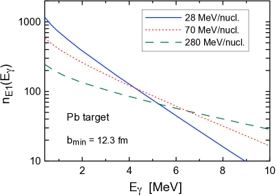
Figure 5: Total number of virtual photons for the $E1$ multipolarity, “as seen” by a projectile passing by a lead target at impact parameters $b_{min}=12.3$ fm and larger (i.e., integrated over impact parameters), for three typical bombarding energies.

The concept of virtual photon numbers is very useful, specially in high energy collisions. In such collisions the momentum and the energy transfer due to the Coulomb interaction are related by $\Delta p=\Delta E/v\simeq\Delta E/c$. This means that the virtual photons are almost real. One usually explores this fact to extract information about real photon processes from the reactions induced by relativistic charges, and vice-versa. This is the basis of the Weizsäcker-Williams method [Fe24,WW34] (it should be called Fermi’s method - see historical note later), used to calculate cross sections for Coulomb excitation, particle production, Bremsstrahlung, etc., (see, e.g., Ref. [Ja75,BB88]).

III.5.3 Virtual and real photons

We have shown that even at low energies the cross sections for Coulomb excitation can be written as a product of equivalent photon numbers and the cross sections induced by real photons. The reason for this is the assumption that Coulomb excitation is a process which involves only collisions for which the nuclear matter distributions do not overlap at any point of the classical trajectory. The excitation of the target nucleus thus occurs in a region where the divergence of the electric field is zero, i.e. $\mathbf{\nabla\cdot E}_{p}\left(t\right)=0$, where $\mathbf{E}_{p}\left(t\right)$ is the electric field generated by the projectile at the target’s position. This condition implies that the electromagnetic fields involved in Coulomb excitation are exactly the same as those involved in the absorption of a real photon [EG88].

III.5.4 Analytical expression for E1 excitations

For the $E1$ multipolarity the orbital integrals, Eq. (100), assumes a particularly simple form. It can be performed analytically for $M=0,\pm 1$ [AW66]. Using these results, one gets the compact expression for the E1 virtual photon numbers

$${\frac{dn_{E1}}{d\Omega}} = {\frac{Z_{p}^{2}\alpha}{4\pi^{2}}}\;\left({\frac{c}{v}}\right)^{2}\;{\epsilon^{4}\;\zeta^{2}}\;\;e^{-\pi{\zeta}}\;\Big{\{}{\frac{\epsilon^{2}-1}{\epsilon^{2}}}\;\left[K_{i{\zeta}}({\epsilon\zeta})\right]^{2}$$ (113)

$$+ \left[K_{i{\zeta}}^{\prime}({\epsilon\zeta})\right]^{2}\Big{\}}\ ,$$

where $K_{i\zeta}$ is the modified Bessel function with imaginary index,

$$K_{i\zeta}(z)={\Gamma(i\zeta+{1\over 2})(2z)^{i\zeta}\over\sqrt{\pi}}\int_{0}^{\infty}dt{\cos t\over(t^{2}+z^{2})^{i\zeta+{1\over 2}}},$$ (114)

$K_{i\zeta}^{\prime}$ is the derivative with respect to its argument.

This result is not particular useful, as one still has to perform a time integration in the equation above. However, as we will see later, the above formula will help us to understand the connection with relativistic Coulomb exctitation.

In Figure 5 we show a calculation (with $E_{\gamma}\equiv E_{x}$ = excitation energy) of the virtual photons for the $E1$ multipolarity, “as seen” by a projectile passing by a lead target at impact parameters equal to and exceeding $b=12.3$ fm, for three typical bombarding energies. As the projectile energy increases, more virtual photons of large energy are available for the reaction. This increases the number of states accessed in the excitation process.

III.6 Higher order corrections and quantum scattering

The results presented in this section are only valid if the excitation is of first-order. For higher-order excitations one has to use the coupled-channels equations (387) of Appendix B, with the excitation amplitudes in each time interval given by Eq. (89). Important cases of applications of Coulomb excitation require a non-perturbative treatment of the collision process. We will discuss some of these cases in later sections.

A full quantum calculation for Coulomb excitation uses scattering waves for the projectile (and target). The cross section in first order perturbation theory is given by Eq. (400) of Appendix B, with the transition matrix element of Eq. (401) given by

$$V_{fi}=<f\mid\mathcal{H}_{int}\mid i>$$

$$= \int\;\left[\rho_{fi}({\bf r})\phi_{\beta\alpha}(\mathbf{r},{\bf r}^{\prime})-\frac{1}{c}\mathbf{j}_{fi}(\mathbf{r})\cdot\mathbf{A}_{\beta\alpha}(\mathbf{r},{\bf r}^{\prime})\right]d^{3}rd^{3}r^{\prime},$$

where $\phi_{\beta\alpha}({\bf r},{\bf r}^{\prime})$ and ${\bf A}_{\beta\alpha}({\bf r},{\bf r}^{\prime})$ being the electromagnetic potential generated by scattering waves $\chi_{\alpha,\beta}({\bf r}^{\prime})$ in the initial and final scattering states, $\alpha$ and $\beta$, respectively.

Instead of the Coulomb gauge, i.e. with the Coulomb potential proportional to $1/|{\bf r}-{\bf r}^{\prime}|$, it is better to adopt the Lorentz gauge, for which the scalar potential is given by [AW75]

$$\phi({\bf r},\mathbf{r}^{\prime})=Z_{p}e\chi_{\beta}^{(-)*}({\bf r}^{\prime}){\frac{e^{i\kappa\mid\mathbf{r-r^{\prime}}(t)\mid}}{\mid\mathbf{r-r^{\prime}}\mid}}\chi_{\alpha}^{(+)}({\bf r}^{\prime}),$$ (116)

and a similar expression for ${\bf A}({\bf r},{\bf r}^{\prime})$, with the expression for the transition current replacing the product of the outgoing and incoming waves, i.e. $\chi_{\beta}^{(-)*}\chi_{\alpha}^{(+)}\rightarrow(\hbar/2i\mu)[\chi^{(-)*}_{\beta}\bm{\nabla}\chi_{\alpha}^{(+)}-\chi^{(+)}_{\alpha}\bm{\nabla}\chi_{\beta}^{(-)*}]$.

In Eq. (116) one uses well-known expressions for Coulomb waves [BD04]. One also uses the expansion

$${\frac{e^{i\kappa\mid\mathbf{r-r^{\prime}}\mid}}{\mid\mathbf{r-r^{\prime}}\mid}}=4\pi\ i\kappa\sum_{LM}j_{L}(\kappa r_{<})Y_{LM}^{\ast}(\hat{\mathbf{r}}_{<})h_{L}(\kappa r_{>})\,Y_{LM}(\hat{\mathbf{r}}_{>})\ ,$$ (117)

where $j_{L}$ ($h_{L}$) denotes the spherical Bessel (Hankel) functions (of first kind), $\mathbf{r}_{>}$ ($\mathbf{r}_{<}$) refers to whichever of $\mathbf{r}$ and $\mathbf{r}^{\prime}$ has the larger (smaller) magnitude. Assuming that the projectile does not penetrate the target, one uses $\mathbf{r}_{>}$ ($\mathbf{r}_{<}$) for the projectile (target) coordinates.

From here on, the calculation is tedious, but straightforward. A detailed description is found in Ref. [AW75]. More insight into this calculation are not useful because on can show that the quantum treatment of the relative motion between the nuclei does not alter the results of the semiclassical calculations for $\eta\gg 1$. Thus, we can safely use the machinery of the previous sections to have an accurate and reliable description of Coulomb excitation at low energies. For collisions at high energies, the distortion of the scattering waves due to the nuclear interaction yield important modifications of the angular distribution of the relative motion. We will discuss this in more details later.

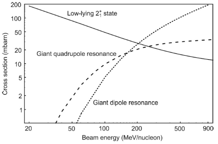
Figure 6: Cross sections for the Coulomb excitation versus incident beam energy for different collective states in the ⁴⁰S$\ +^{197}$Au reaction, assuming a minimum impact parameter $b_{\min}=16$ fm (from Ref. [Gla01]).

As the bombarding energy increases Coulomb excitation predominantly favors the excitation of high lying states, e.g. giant resonances. This is shown in figure 6 for the cross sections of Coulomb excitation versus incident beam energy for different collective states in the ⁴⁰S$\ +^{197}$Au reaction, assuming a minimum impact parameter $b_{\min}=16$ fm. Later we will discuss more about the excitation of giant resonances.

IV Angular distribution of $\gamma$-rays

Coulomb excitation is a useful method to obtain static quadrupole moments as well as the reduced probabilities for several nuclear transitions. In order to identify the multipolarity of the excitation it is often necessary to study the de-excitation of the excited state by measuring a $\gamma$-ray from its decay (see figure 7).

A detailed description of $\gamma$-ray emission following excitation is give in Appendix E. The angular distribution of the gamma rays emitted into solid angle $\Omega_{\gamma}$, as a function of the scattering angle of the projectile $\vartheta$, is given by Eq. (488), i.e.,

$$W(\theta_{\gamma})=1+\sum_{k=2,4,...}b_{k}^{\pi L}\left(\vartheta\right)P_{k}\left(\cos\theta_{\gamma}\right)\ ,$$ (118)

where $P_{k}\left(\cos\theta_{\gamma}\right)$ are the Legendre polynomials. The coefficients $b_{k}^{\pi L}\left(\vartheta\right)$ are related to the Coulomb excitation amplitudes (89) and to the B-values (35) for the transition from the excited state $f$ to a final state $g$.

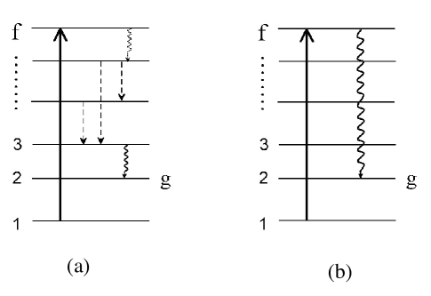
Figure 7: Schematic description of a nuclear excitation (solid line) followed by $\gamma$-decay (solid wavy line). (a) The dashed lines are transitions due to internal conversion (unobserved). The dashed wavy line is an unobserved $\gamma$-decay. (b) Direct emission of an observed gamma ray.

Figure 8 shows the Coulomb excitation of sodium by protons. The yield of the 446 keV $\gamma$-rays is shown [Tem55]. Between the resonances due to compound nucleus formation one observes a smoothly rising background yield which may be ascribed to Coulomb excitation. It is possible to determine the multipole order of the Coulomb excitation by comparing with the yield observed in the Coulomb excitation with $\alpha$-particles [Tem55]. The dashed curves correspond to the cross sections expected for $L=1$ and 2 on the basis of the observed cross section for the excitation with $\alpha$-particles. The close agreement of the measured cross section with the theoretical curve for $E2$ excitation also confirms that the yield away from resonances is primarily due to Coulomb excitation.

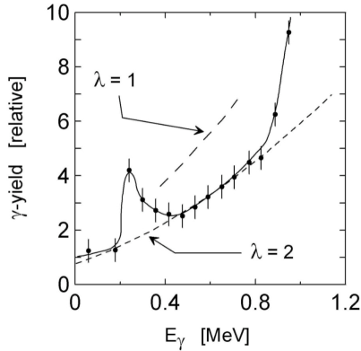
Figure 8: Coulomb excitation of sodium by protons. The yield of the 446 keV $\gamma$-rays is shown [Tem55]. The dashed curves correspond to the cross sections expected for $L=1$ and 2 on the basis of the observed cross section for the excitation with $\alpha$-particles.

Figure 9 shows the $\gamma$-ray yield from Coulomb excitation and compound nucleus formation in ¹⁹F bombarded with $\alpha$-particles. The dashed curve shows the yields of the 114 keV $\gamma$-ray from the first excited state in ¹⁹F and the solid curve shows the 1.28 MeV $\gamma$-ray from the first excited state of ²²Ne formed by an $\left(\alpha,\text{p'}\right)$ process on ¹⁹F [She54]. For bombarding energies  below 1.2 MeV, the penetration of the $\alpha$-particle through the Coulomb barrier is very small and the cross section for compound nucleus formation is small compared to that for Coulomb excitation. With increasing energy, the cross section for compound nucleus formation, $\sigma_{\mathrm{CN}}$, increases rapidly and soon becomes larger than the Coulomb excitation cross section, $\sigma_{C}$. However, even for $E_{\alpha}\sim 2$ MeV, at which energy the average value of $\sigma_{\mathrm{CN}}$ is an order of magnitude larger than $\sigma_{C}$, the yield of the 114 keV $\gamma$-ray is only very little affected by the compound nucleus formation, since the probability that the compound nucleus decays by inelastic $\alpha$-emission is small. Finally, for $E_{\alpha}\geq 2$ MeV, the Coulomb excitation yield of the 114 keV $\gamma$-ray is overshadowed by the resonance yield from compound nucleus formation.

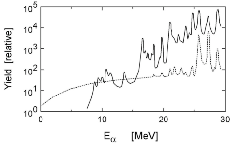
Figure 9: $\gamma$-rays from Coulomb excitation and compound nucleus formation in ¹⁹F bombarded with $\alpha$-particles. The dashed curve shows the yields of the 114 keV $\gamma$-ray from the first excited state in ¹⁹F and the solid curve shows the 1.28 MeV $\gamma$-ray from the first excited state of ²²Ne formed by an $\left(\alpha,\text{p'}\right)$ process on ¹⁹F [She54].

V Relativistic collisions

V.1 Multipole expansion

When the projectile has very high energies, e.g. $E_{lab}>100$ MeV/nucleon, there is very little deflection of the ion trajectory. The recoil by the target is also minimal. We thus assume that the projectile moves on a straight-line trajectory of impact parameter $b$, which is also the distance of closest approach between the centers of mass of the two nuclei at time $t=0$. We will consider the situation where $b$ is larger than the sum of the two nuclear radii, $R$, such that the charge distributions of the two nuclei do not overlap at any time. We will use a coordinate system with origin in the center of mass of the excited nucleus and with z-axis along the projectile velocity $v$, which is assumed to be constant. In this coordinate system the electromagnetic field from this other nucleus is given by the Lienard-Wiechert expression

$$\phi\left(\mathbf{r},t\right)=\frac{\gamma Ze}{\sqrt{(x-b)^{2}+y^{2}+\gamma^{2}(z-vt)^{2}}}.$$ (119)

We have chosen the x-axis in the plane of the trajectory such that the x-component of the trajectory is $b$. This expression reduces to the non-reletivistic Coulomb field of an low energy charge given by $={Ze}/{\mid\mathbf{r}-\mathbf{R}(t)\mid}$. The appearance of the factors $\gamma=(1-v^{2}/c^{2})^{-1/2}$ are due to retardation (see [Ja75]). The vector potential is

$$\mathbf{A}(\mathbf{r},t)=\frac{\mathbf{v}}{c}\phi(\mathbf{r},t),$$ (120)

with ${\bf v}=v\hat{\bf z}$ being a constant velocity vector.

The procedure for obtaining the excitation amplitude in (78) should be the same as adopted before: first we make a multipole expansion of (119), then we separate the intrinsic from the relative motion coordinates, and perform the time integrals for the trajectories (we named them orbital integrals). However, as shown in Ref. [AW79], it is better to first calculate the time integrals and then perform the multipole expansion. In fact, this seems to be the only way to get analytical expressions, except when one uses a more complicated approach as we will discuss later.

The integral in Eq. (80) yields

$$\phi(\mathbf{r},\omega)={2Ze\over v}e^{i\omega v/z}K_{0}\left({\omega\over v}q\right),$$ (121)

where $K_{0}$ is a modified Bessel function and

$$q={1\over\gamma^{2}}\left[(b-x)^{2}+y^{2}\right].$$ (122)

In Ref. [AW79] it was shown that the multipole expansion of (121) is given by

$$\phi(\mathbf{r},\omega)=\sum_{LM}W_{LM}({\bf r},\omega)Y^{\ast}_{LM}(\hat{\bf r}),$$ (123)

with

$$W_{LM}({\bf r},\omega)=\sqrt{16\pi(2L+1)}\left({(L-M)!\over(L+M)!}\right)^{1/2}(2M-1)!!$$

$$\times i^{L+M}{Ze\over v}\left({c\over\gamma v}\right)^{M}K_{M}\left({\omega b\over\gamma v}\right)C_{L-M}^{M+1/2}\left({c\over v}\right)j_{L}({\kappa r}).$$

The quantity $C_{M}^{N}(x)$ is the Gegenbauer polynomial [AS64], while $j_{m}(\kappa r)$ is a spherical Bessel function, with $\kappa=\omega/c$. For $M<0$,

$$W_{L,-M}({\bf r},\omega)=(-1)^{M}W_{LM}({\bf r},\omega)$$ (125)

After separation of the internal degrees of freedom, one gets [AW79]

$$a_{fi} = -i{Ze\over\hbar v\gamma}\sum_{\pi LM}G_{\pi LM}\left({c\over v}\right)(-1)^{M}K_{M}\left({\omega b\over\gamma v}\right)$$ (126)

$$\times \sqrt{2L+1}\kappa^{L}{\cal M}_{fi}(\pi L,-M)$$

where the transition matrix elements are given by ${\cal M}_{fi}(\pi L,-M)$ are given by Eqs. (III.4) and (91).

The functions $G_{\pi LM}$ have analytical expressions [WA79]. For the $E1$, $E2$, $E3$, $M1$ and $M2$ multipolarities, they are given by

$$G_{E10}(x) = -i{4\over 3}\sqrt{\pi(x^{2}-1)};$$

$$G_{E11}(x) = -G_{E1-1}(x)={1\over 3}x\sqrt{8\pi};$$

$$G_{M11}(x) = G_{M1-1}(x)=-i{1\over 3}\sqrt{8\pi};\ \ \ G_{M10}(x)=0;$$

$$G_{E22}(x) = G_{E2-2}(x)=-{2\over 5}x\sqrt{{\pi\over 6}(x^{2}-1)};$$

$$G_{E21}(x) = -G_{E2-1}(x)=i{2\over 5}\sqrt{\pi\over 6}(2x^{2}-1);\ \ \$$

$$G_{E20}(x) = {2\over 5}x\sqrt{\pi(x^{2}-1)};$$

$$G_{M22}(x) = -G_{M2-2}(x)=i{2\over 5}\sqrt{\pi\over 6}\sqrt{x^{2}-1};$$

$$G_{M21}(x) = G_{M2-1}(x)={2\over 5}x\sqrt{\pi\over 6};\ \ \ G_{M20}=0;$$

$$G_{E33}(x) = -G_{E3-3}(x)={1\over 21}\sqrt{\pi\over 5}x(x^{2}-1);$$

$$G_{E32}(x) = G_{E3-2}(x)=-i{1\over 21}\sqrt{2\pi\over 15}(3x^{2}-1)\sqrt{x^{2}-1};$$

$$G_{E31}(x) = -G_{E3-1}(x)=-{1\over 105}\sqrt{\pi\over 3}x(15x^{2}-11)$$

$$G_{E30}(x) = i{2\over 105}\sqrt{\pi}(5x^{2}-1)\sqrt{x^{2}-1}.$$

From the excitation amplitude (126) one finds the total cross section for exciting the nuclear state of spin $I_{f}$ in collisions with impact parameters larger than $R$ given by,

$$\sigma_{fi} = \left({Ze\over\hbar c}\right)^{2}\sum_{\pi LM}\kappa^{2(L-1)}B(\pi L,I_{i}\rightarrow I_{f})$$ (128)

$$\times \left|G_{\pi LM}\left({c\over v}\right)\right|^{2}g_{M}\left(\xi(R)\right),$$

where

$$\xi(R)={\omega R\over\gamma v},$$ (129)

and, for $M\geq 0$,

$$g_{M}(\xi) = g_{-M}(\xi)=2\pi\left({\omega\over\gamma v}\right)^{2}\int_{R}^{\infty}db\ b\ K_{M}^{2}\left(\xi(b)\right)$$ (130)

$$= \pi\xi^{2}\left[K_{M+1}^{2}-K_{M}^{2}-{2M\over\xi}K_{M+1}K_{M}\right],$$

where all $K_{M}$’s are functions of $\xi(b)={\omega b/}\gamma v$.

V.2 Excitation probabilities and virtual photon numbers

The theoretical results for relativistic Coulomb excitation can be rewritten in terms of the virtual photon numbers, as shown in Ref. [BB85]. The probability for exciting the nuclear state of energy $I_{f}$ is obtained directly from Eq. (126) by using

$$P_{fi}={\frac{1}{2I_{i}+1}}\;\sum_{M_{i},M_{f}}\mid a_{fi}\mid^{2}.$$ (131)

As with the low-energy case, we can rewrite the final result in terms of the reduced transition probabilities for photo-excitation. It can be cast in the form

$$P_{fi}(b,E_{\gamma}) = \sum_{\pi L}\;P_{\pi L}(b,E_{\gamma})$$

$$= \sum_{\pi L}\int{\frac{dE_{\gamma}}{E_{\gamma}}}\;n_{\pi L}(E_{\gamma},b)\;\sigma_{\gamma}^{\pi L}(E_{\gamma}),$$

where $\sigma_{\gamma}^{\pi L}(E_{\gamma})$ is the photonuclear absorption cross sections for a given multipolarity $\pi L$ given by Eq. (105). The total photonuclear cross section is a sum of all these multipolarities,

$$\sigma_{\gamma}=\sum_{\pi L}\sigma_{\gamma}^{\pi L}(E_{\gamma})\,.$$ (133)

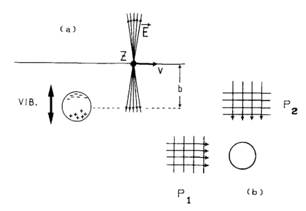
Figure 10: (a) A relativistic charged projectile incident on a target with impact parameter larger than the strong interaction radius. A sketch of the electric field generated by it is also shown. One of the effects of this field is to induce collective vibrations of the nuclear charges. (b) Two pulses of plane wave of light which produce the same effect on the target as the electromagnetic field created by the projectile’s motion. (from [BB88]).

The functions $n_{\pi L}(E_{\gamma})$ are called the virtual photon numbers, and are given by [BB85]

$$n_{E1}(b,E_{\gamma}) = {\frac{Z^{2}\alpha}{\pi^{2}}}\,{\frac{\xi^{2}}{b^{2}}}\,({\frac{c}{v}})^{2}\,\left\{K_{1}^{2}+{\frac{1}{\gamma^{2}}}\,K_{0}^{2}\right\},$$ (134)

$$n_{E2}(b,E_{\gamma}) = {\frac{Z^{2}\alpha}{\pi^{2}b^{2}}}\,({\frac{c}{v}})^{4}\,\Bigg{\{}{\frac{4}{\gamma^{2}}}\,\left[K_{1}^{2}+\xi K_{0}K_{1}+\xi^{2}K_{0}^{2}\right]$$ (135)

$$+ \xi^{2}(2-v^{2}/c^{2})^{2}K_{1}^{2}\Bigg{\}},$$

$$n_{M1}(b,E_{\gamma}) = {\frac{Z^{2}\alpha}{\pi^{2}}}\,{\frac{\xi^{2}}{b^{2}}}\,K_{1}^{2},$$ (136)

where all $K_{M}$’s are functions of $\xi(b)={\omega b/}\gamma v$.

Since all nuclear excitation dynamics is contained in the photoabsorption cross section, the virtual photon numbers, Eqs. (134), (135) and (136), do not depend on the nuclear structure. They are kinematical factors, depending on the orbital motion. They may be interpreted as the number of equivalent (virtual) photons that hit the target per unit area.

The cross section is obtained by the impact parameter integral of the excitation probabilities. Eq. (LABEL:(4.5a)) shows that we only need to integrate the number of virtual photons over impact parameter. One has to introduce a minimum impact parameter $b_{0}$ in the integration. Impact parameters smaller than $b_{0}$ are dominated by nuclear fragmentation processes. One finds

$$\sigma_{C}=\sum_{\pi L}\;\sigma_{\pi L}=\sum_{\pi L}\int{\frac{dE_{\gamma}}{E_{\gamma}}}\;N_{\pi L}(E_{\gamma})\;\sigma_{\gamma}^{\pi L}(E_{\gamma})\,,$$ (137)

where the total virtual photon numbers $N_{\pi L}(E_{\gamma})=2\pi\int db\ b\ n_{\pi L}(b,E_{\gamma})$ are given analytically by

$$N_{E1}(E_{\gamma}) = {\frac{2Z^{2}\alpha}{\pi}}\,({\frac{c}{v}})^{2}\,\left[\xi K_{0}K_{1}-{\frac{v^{2}\xi^{2}}{2c^{2}}}\,(K_{1}^{2}-K_{0}^{2})\right],$$

$$N_{E2}(E_{\gamma}) = {\frac{2Z^{2}\alpha}{\pi}}\,({\frac{c}{v}})^{4}\,\Big{[}{2\over\gamma^{2}}K_{1}^{2}+{\xi\over\gamma^{4}}K_{0}K_{1}$$

$$+{\frac{\xi^{2}v^{4}}{2c^{4}}}(K_{1}^{2}-K_{0}^{2})+\xi^{2}(2-v^{2}/c^{2})^{2}K_{1}^{2}\Big{]},$$

$$N_{M1}(E_{\gamma}) = {\frac{2Z^{2}\alpha}{\pi}}\,{\frac{\xi^{2}}{R^{2}}}\,\left[\xi K_{0}K_{1}-{\frac{\xi^{2}}{2}}\,(K_{1}^{2}-K_{0}^{2})\right],$$

where all $K_{M}$’s are now functions of $\xi(R)={\omega R/}\gamma v$

The usefulness of Coulomb excitation, even in first order processes, is displayed in Eq. (LABEL:(4.5a)). The field of a real photon contains all multipolarities with the same weight and the photonuclear cross section, Eq. (133) is a mixture of the contributions from all multipolarities, although only a few contribute in most processes. In the case of Coulomb excitation the total cross section is weighted by kinematical factors which are different for each projectile or bombarding energy. This allows one to disentangle the multipolarities when several ones are involved in the excitation process, except for the very high bombarding energies $\gamma\gg 1$ for which all virtual photon numbers can be shown to be all the same [BB85] to

$$n_{\pi L}={2\over\pi}Z^{2}\alpha\ln\left({\delta\over\xi}\right).$$ (141)

Since $\xi=\omega R/\gamma c\ll 1$, we have a logarithmic rise of the cross section for all multipolarities with $\gamma$. The impinging projectile acts like a spectrum of plane wave photons with helicity $m=\mp 1$. Such a photon spectrum contains equally all multipolarities $\pi L$.

V.3 Historical note: Fermi’s forgotten papers

In 1924, Enrico Fermi, then 23 years old, submitted a paper “On the Theory of Collisions Between Atoms and Elastically Charged Particles to Zeitschrift für Physik [Fe24]. This paper does not appear in his “Collected Works. Nevertheless, it is said that this was one of Fermi s favorite ideas and that he often used it later in life. In this publication, Fermi devised a method known as the equivalent (or virtual) photon method, where he treated the electromagnetic fields of a charged particle as a flux of virtual photons. It is also interesting that Fermi published the same paper, but in the Italian language, in Nuovo Cimento [Fe25] (it is rather uncommon that the same paper is published twice!). Ten years later, Weiszsäcker and Williams [WW34] extended this approach to include ultra-relativistic particles, basically restoring the Lorentz $\gamma$ factors in the right places. However, it is indisputable that Fermi’s papers [Fe24,Fe25] introduced the ingenious virtual photon method.

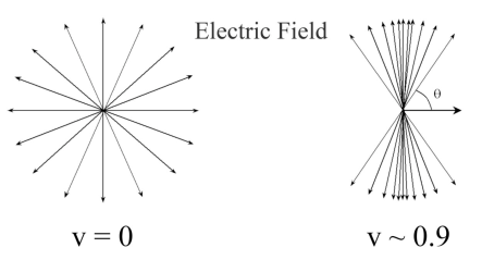
Figure 11: Left: Electric field of a slowly moving charge. Right: Electric field of a charge moving with $v=0.9$ (in units of $c$).

A fast-moving charged particle has electric field vectors pointing radially outward and magnetic fields circling it. The field at a point some distance away from the trajectory of the particle resembles that of a real photon. Thus, Fermi replaced the electromagnetic fields from a fast particle with an equivalent flux of photons, as shown schematically in figure 10.

Fermi’s virtual photon method is based on the idea that, when $v\sim c$, where $c$ is the velocity of light, the electromagnetic field generated by the projectile looks contracted in the direction perpendicular to its motion (see figures 11 and 12) and is given by

$$E_{z} = -{Ze\gamma vt\over(b^{2}+\gamma^{2}v^{2}t^{2})^{3/2}},$$

$${\bf E}_{T} = {Ze\gamma{\bf b}\over(b^{2}+\gamma^{2}v^{2}t^{2})^{3/2}},$$

$${\bf B}_{T} = {{\bf v}\over c}\otimes{\bf E}_{T},\ \ \ \ {\rm and}\ \ B_{z}=0.$$ (142)

where the $z$ ($T$) indices denote the direction parallel (transverse) to the velocity of the projectile.

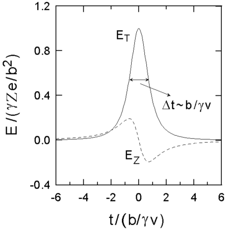
Figure 12: Longitudinal and transverse electric field of a straight-line moving charge at high energies as a function of time. Both variables are gauged in appropriate units, as sown in the axis labels.

When $\gamma\gg 1$, these fields will act during a very short time, of order

$$t={b\over\gamma v}\simeq{b\over\gamma c},$$ (143)

and they are equivalent to two pulses of plane-polarized radiation incident on the target (see fig. 10): one in the beam direction (P1), and the other perpendicular to it (P2). In the case of the pulse P1 the equivalency is exact. Since the electric field in the $z$-direction is not accompanied by a corresponding magnetic field, the equivalency is not complete for pulse P2, but this will not appreciably affect the dynamics of the problem since the effects of the field $E_{z}$ are of minor relevance when v = c. Therefore, we add a field $B=vE_{z}/c$ to Eq. (142) in order to treat also P2 as a plane-wave pulse of radiation. This analogy permits one to calculate the amount of energy incident on the target per unit area and per by Fourier transforming the Poynting vector ${\bf S}={\bf E}\otimes{\bf B}$ and calculating the intensity of the virtual radiation, $I(\omega,b$), with $E_{\gamma}=\hbar\omega$. This procedure is nicely explained in Ref. [Ja75].

Fermi associated the spectrum of the virtual radiation as described above to the one of a real pulse of light incident on the target. Then he obtained the probability for nuclear (in fact, Fermi was interested in atomic transitions) by a fast charge, in terms of the cross sections for the same process generated by an equivalent pulse of light, i.e.

$$P(b)=\int I(\omega,b)\sigma_{\gamma}(E_{\gamma})dE_{\gamma}=\int n(\omega,b)\sigma_{\gamma}(E_{\gamma}){d\omega\over\omega},$$

where $\sigma_{\gamma}(E_{\gamma})$ is the photo cross-section for the photon energy $E_{\gamma}$, and the integral runs over all the frequency spectrum of the virtual radiation. The quantities $n(\omega,b)$ can be interpreted as the number of equivalent photons incident on the target per unit area.

Following this procedure, Fermi obtained the Eq. (134) for $n(\omega,b)\equiv n_{E1}(\omega,b)$, without the $\gamma$ factors (Fermi was not interested in relativistic collisions in 1924!). The $\gamma$ factors were found in the proper places by Weizsäcker and Williams [WW34]. It is somewhat surprising that Fermi, Weizsäcker, and Williams obtained the “exact” result of the virtual photons for the $E1$ multipolarity. Their method was completely classical and approximate (in adding the $B_{z}$ field). To reach Eq. (134) some quantum mechanics was used (e.g., the continuity equation for the nuclear transitions). Eq. (134) is also the result of a multipole expansion, which was not used in the classical prescription. In fact, the Eqs. (134-136) are an improvement of Fermi’s method for higher multipolarities, and were obtained in Ref. [BB85]. As we show later, a quantum mechanical description of high-energy scattering leads to the same expressions in Eqs. (134-136).

V.4 Spectrum of virtual photons

In Eq. (134) the first term inside parentheses comes from the contribution of the pulse P1, whereas the second term comes from the contribution of the pulse P2. One immediately sees that the contribution of pulse P2 becomes negligible for $\gamma\gg 1$. The shape of the equivalent photon spectrum for a given impact parameter can be expressed in terms of the dimensionless function $\phi(x)=x^{2}K^{2}_{1}(x)$, if we neglect the pulse P2. In a crude approximation, $\phi\sim 0$ for $x>1$, and $\phi=1$ for $x<1$. This reflects in a sudden cutoff of the virtual photon spectra, as can be seen from figure 13. This implies that, in a collision with impact parameter $b$, the spectrum will contain equivalent photons with energies up to a maximum value of order

$$E^{\max}_{\gamma}\simeq{\gamma\hbar v\over b},$$ (144)

which we call by adiabatic cutoff energy. This means that in an electromagnetic collision of two nuclei the excitation of states with energies up to the above value can be reached. We can explain this result by observing that in a collision with interaction time given by Eq. (143) only states satisfying the condition $T/\Delta t\gg 1$, where $T$ is the period of the quantum states, will have an appreciable chance to be excited. Otherwise, the quantum system will respond adiabatically to the interaction. In a collision with a typical impact parameter of $b10$ fm one can reach states with energy around $E_{\max}\sim 20\gamma$ MeV. Among the many possibilities, we cite the following: for $E_{\gamma}=10-20$ MeV (already small values of $\gamma$), excitation of giant resonances, with subsequent nucleon emission; for $E=20-100$ MeV, the quasideuteron effect which corresponds to a photon absorption of a correlated N-N pair in the nucleus; and for $E_{\gamma}>100$ MeV, pion production through A-isobar excitation which has a maximum at $E\simeq 200$ MeV. Also the production of lepton pairs ($e^{+}e^{-}$, $q\hat{q}$ (mesons), etc.) are accessible with increasing value of $\gamma$.

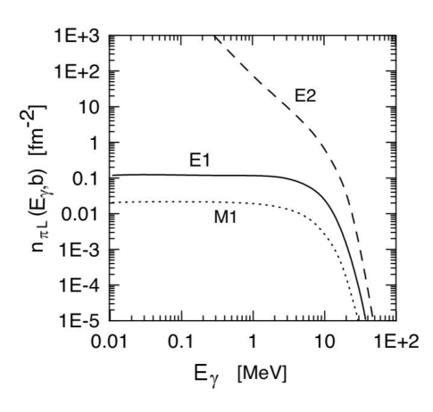
Figure 13: Equivalent photon numbers per unit area incident on ²⁰⁸Pb, in a collision with ¹⁶O at 100 MeV/nucleon and with impact parameter $b=15$ fm, as a function of the photon energy $E=\hbar\omega$. The curves for the E1, E2 and M1 multipolarities are shown.

In figure 14 we show $n_{\pi L}$ (with $Z={\rm unity}$) as given by Eqs. (134-136), as a function of $\omega R/c$. We see that $n_{E2}\simeq n_{E1}\simeq n_{M1}$ for small values of $\gamma$, in contrast to the limit $\gamma\sim 1$. The physical reason for these two different behaviours of the equivalent photon spectrum is the following. The electric field of a charged particle moving at low energies is approximately radial and the lines of force of the field are isotropically distributed, with their relative spacing increasing with the radial distance (see figure 11). When interacting with a target of finite dimension, the non-uniformity of the field inside the target is responsible for the large electric quadrupole interaction between them. The same lines of force of an ultrarelativistic ($\gamma\gg 1$) charged particle appear more parallel and compressed in the direction transverse to the particle’s motion, due to the Lorentz contraction (see figure 11). As seen from the target, this field looks like a pulse of a plane wave. But plane waves contain all electric and magnetic multipolarities with the same weight. This is the cause for the equality between the equivalent photon numbers as $\gamma\rightarrow\infty$.

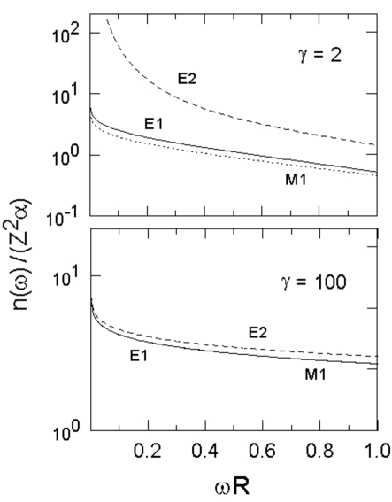
Figure 14: Equivalent photon number per unit projectile charge, for El, M1 and E2 radiation, and as a function of the ratio between $R$ and the photon wavelength. $\gamma$ is the ratio of the projectile energy to its rest energy. (Here, $c=1$.)

VI Quantum treatment of relativistic Coulomb excitation

In contrast to sub-barrier Coulomb excitation, at relativistic energies the effects of the nuclear interaction are visible due to the distortion it causes on the scattered waves. Fortunately, at high energies, this can be treated in a simple manner by using the eikonal approximation. Our discussion will be general, with very little emphasis on the details of the nuclear interaction.

VI.1 The eikonal wavefunction

The free-particle wavefunction

$$\psi\sim e^{i\mathbf{k}\cdot\mathbf{r}}$$ (145)

becomes “distorted” in the presence of a potential $\,V(\mathbf{r}\,)\,$. The distorted wave can be calculated numerically by performing a partial wave-expansion [Ber07] solving the Schrödinger equation for each partial wave, i.e.

$$\left[\frac{d^{2}}{dr^{2}}+k_{l}^{2}(r)\right]\chi_{l}(r)=0\;,$$ (146)

where

$$k_{l}(r)=\left\{\frac{2\mu}{\hbar^{2}}\left[E-V(r)-\frac{l(l+1)\hbar^{2}}{2\mu r^{2}}\right]\right\}^{1/2}.$$ (147)

with the condition that asymptotically $\,\psi(\mathbf{r}\,)$ behaves as (145).

The solution of (146) involves a great numerical effort at large bombarding energies $\,E\,$. Fortunately, at large energies $\,E\,$ a very useful approximation is valid when the excitation energies $\,\Delta E\,$ are much smaller than $\,E\,$ and the nuclei (or nucleons) move in forward directions, i.e., $\,\theta\ll 1\,$.

Calling $\,\mathbf{r}=(z,\mathbf{b}\,)$, where $\,z\,$ is the coordinate along the beam direction, we can assume that

$$\psi(\mathbf{r}\,)=e^{ikz}\,\phi(z,\mathbf{b}\,),$$ (148)

where $\,\phi\,$ is a slowly varying function of $\,z\,$ and $\,b\,$, so that

$$\left|\nabla^{2}\phi\,\right|\ll\,k\left|\nabla\phi\right|.$$ (149)

In cylindrical coordinates the Schrödinger equation

$$-\frac{\hbar^{2}}{2\mu}\nabla^{2}\psi(\mathbf{r}\,)+V(\mathbf{r}\,)\psi(\mathbf{r}\,)=E\,\psi(\mathbf{r}\,)$$

becomes

$$2ik\,e^{ikz}\frac{\partial\phi}{\partial z}+e^{ikz}\frac{\partial^{2}\phi}{\partial z^{2}}+e^{ikz}\,\nabla_{b}^{2}\phi-\frac{2m}{\hbar^{2}}\,V\,e^{ikz}\,\phi=0$$

or, neglecting the 2nd and 3rd terms because of (149),

$$\frac{\partial\phi}{\partial z}=-\frac{i}{\hbar\mathrm{v}}V(\mathbf{r}\,)\phi$$ (150)

whose solution is

$$\phi=\exp\left\{-\frac{i}{\hbar\mathrm{v}}\int_{-\infty}^{z}\,V(\mathbf{b},z^{\prime})dz^{\prime}\right\}.$$ (151)

That is,

$$\psi(\mathbf{r})=\exp\left\{ikz+i\chi(\mathbf{b},z)\right\},$$ (152)

where

$$\chi(\mathbf{b},z)=-\frac{1}{\hbar\mathrm{v}}\int_{-\infty}^{z}\,V(\mathbf{b},z^{\prime})dz^{\prime}$$ (153)

is the eikonal phase. Given $\,V(\mathbf{r}\,)\,$ one needs a single integral to determine the wavefunction: a great simplification of the problem.

The eikonal approximation, in the same form as given by eqs. (152), can be obtained from the Klein-Gordon equation with a (scalar) potential$\,V$. We will use this approximation in several discussions later on this review.

VI.2 Quantum relativistic Coulomb excitation

Defining r as the separation between the center of mass of the two nuclei and r^′ as the intrinsic coordinate of the target nucleus, the inelastic scattering amplitude to first-order is given by [BD04]

$$f(\theta) = {\frac{ik}{2\pi\hbar v}}\ \int d^{3}r\ d^{3}r^{\prime}$$

$$\left<\Phi_{\mathbf{k^{\prime}}}^{(-)}(\mathbf{r})\ \phi_{f}(\mathbf{r}^{\prime})\ \left|\ {\cal H}_{int}(\mathbf{r},\ \mathbf{r}^{\prime})\ \right|\ \Phi_{\mathbf{k}}^{(+)}(\mathbf{r})\ \phi_{i}(\mathbf{r}^{\prime})\right>,$$

where $\Phi_{\mathbf{k^{\prime}}}^{(-)}(\mathbf{r})$ and $\Phi_{\mathbf{k}}^{(+)}(\mathbf{r})$ are the incoming and outgoing distorted waves, respectively, for the scattering of the center of mass of the nuclei, and $\phi(\mathbf{r}^{\prime})$ is the intrinsic nuclear wavefunction of the target nucleus.

At intermediate energies, $\Delta E/E_{lab}\ll 1$, and forward angles, $\theta\ll 1$, we can use eikonal wavefunctions for the distorted waves; i.e.,

$$\Phi_{\mathbf{k^{\prime}}}^{(-)\ast}(\mathbf{r})\ \Phi_{\mathbf{k}}^{(+)}(\mathbf{r})=\exp\left\{-i\mathbf{q.r}+i\chi(b)\right\}\;,$$ (155)

where

$$\chi(b)=-{\frac{1}{\hbar v}}\int_{-\infty}^{\infty}U_{N}^{opt}(z^{\prime},\ b)\ dz^{\prime}+i\chi_{C}(b)$$ (156)

is the eikonal-phase, $\mathbf{q}=\mathbf{k}^{\prime}-\mathbf{k}$, $U_{N}^{opt}$ is the nuclear optical potential, and $\chi_{C}(b)$ is the Coulomb eikonal phase,

$$\chi_{C}(b)=\frac{2Z_{p}Z_{t}e^{2}}{\hbar\mathrm{v}}\,\ln(kb)\ ,$$ (157)

where $Z_{p}$ ($Z_{t}$) is the projectile (target) nuclear charges. The Coulomb phase, as given by the above formula, reproduces the Coulomb amplitude for the scattering of point particles in the eikonal approximation for elastic scattering [BD04]. Corrections due to the extended nuclear charges can be easily incorporated [BD04]. Here we have defined the impact parameter b as $\mathbf{b}=\mathbf{r}\times\hat{\mathbf{z}}$.

In Eq. (LABEL:fth) the interaction potential, assumed to be purely Coulomb, is given by Eqs. (LABEL:(higho1)) and (116). Performing the multipole expansion as in Eq. (117), one finds [BN93]

$$f_{C}({\theta}) =i{\frac{Zek}{\gamma\hbar v}}\sum_{\pi LM}i^{M}\left({\frac{\omega}{c}}\right)^{L}\sqrt{2L+1}\ e^{-iM\phi}$$

$$\times\Omega_{M}(q)\ G_{\pi LM}\left({\frac{c}{v}}\right)\left<I_{f}\ M_{f}\ |\ \mathcal{M}(\pi L,\ -M)\ |I_{i}\ M_{i}\right>$$ (158)

where the functions $G_{\pi LM}$ are given in Eq. (V.1). The function $\Omega_{m}(q)$ is given by [BN93]

$$\Omega_{M}(q)=\int_{0}^{\infty}db\ b\ J_{M}(qb)\ K_{M}\left({\frac{\omega b}{\gamma v}}\right)\ \exp\left\{i\chi(b)\right\}\;,$$ (159)

where $q=2k\sin(\theta/2)$ is the momentum transfer, $\theta$ and $\phi$ are the polar and azimuthal scattering angles, respectively.

In the sharp-cutoff approximation, one assumes

$$\exp\left\{i\chi(b)\right\} = 0,\ \ \ {\rm if}\ \ b\leq R,$$ (160)

$$= 1,\ \ \ {\rm if}\ \ b>R,$$

where $R$ is the strong interaction radius, or minimum impact parameter. Then the integral (159) can be performed analytically [BB85].

Using techniques similar to those discussed in previous sections, one obtains

$${\frac{d^{2}\sigma_{C}}{d\Omega\,dE_{\gamma}}}\ \left(E_{\gamma}\right)={\frac{1}{E_{\gamma}}}\ \sum_{\pi L}{\frac{dn_{\pi L}}{d\Omega}}\ \sigma_{\gamma}^{\pi L}\ \left(E_{\gamma}\right)$$ (161)

where d $dn_{\pi L}/d\Omega$ is the virtual photon number given by [BN93]

$${\frac{dn_{\pi L}}{d\Omega}} = Z^{2}\alpha\ \left({\frac{\omega k}{\gamma v}}\right)^{2}{\frac{L\left[(2L+1)!!\right]^{2}}{(2\pi)^{3}\ (L+1)}}$$ (162)

$$\times \sum_{M}|G_{\pi LM}|^{2}\ |\Omega_{M}(q)|^{2}.$$

The total cross section for Coulomb excitation can be obtained from eqs. (161) and (162), using the approximation $d\Omega\simeq 2\pi qdq/k^{2}$, valid for small scattering angles and small energy losses. Using the closure relation for the Bessel functions,

$$\int dq\ qJ_{M}{qx}J_{M}(qx^{\prime})={1\over x}\delta(x-x^{\prime}),$$ (163)

one obtains

$${\frac{d\sigma_{C}}{dE_{\gamma}}}\ \left(E_{\gamma}\right)={\frac{1}{E_{\gamma}}}\ \sum_{\pi L}N_{\pi L}\left(E_{\gamma}\right)\ \sigma_{\gamma}^{\pi L}\ \left(E_{\gamma}\right)\;,$$ (164)

where the total number of virtual photon with energy $\hbar\omega$ is given by

$$N_{\pi L}(\omega)=Z^{2}\alpha\ {\frac{L\left[(2L+1)!!\right]^{2}}{(2\pi)^{3}\ (L+1)}}\ \sum_{m}\ |G_{\pi LM}|^{2}\ g_{M}(\omega)\;,$$ (165)

and

$$g_{M}(\omega)=2\pi\ \left({\frac{\omega}{\gamma v}}\right)^{2}\ \int db\ b\ K_{M}^{2}\left({\frac{\omega b}{\gamma v}}\right)\ \exp\left\{-2\ \chi_{I}(b)\right\}\;,$$ (166)

where $\chi_{I}(b)$ is the imaginary part of $\chi(b)$, which is obtained from Eq.  (156) and the imaginary part of the optical potential.

If one uses the sharp-cutoff approximation, Eq. (160), one recovers the result in Eq. (130) [BB85].

We point out that for very light heavy ion partners, the distortion of the scattering wavefunctions caused by the nuclear field is not important. This distortion is manifested in the diffraction peaks of the angular distributions, characteristic of strong absorption processes. If $Z_{p}Z_{t}\alpha\gg 1$, one can neglect the diffraction peaks in the inelastic scattering cross sections and a purely Coulomb excitation process emerges. One can gain insight into the excitation mechanism by looking at how the semiclassical limit of the excitation amplitudes emerges from the general result (162).

VI.3 Semiclassical limit of the Coulomb excitation amplitudes

If we assume that Coulomb scattering is dominant and neglect the nuclear phase in Eq.  (156), we get

$$\Omega_{M}(q)\simeq\int_{0}^{\infty}db\ b\ J_{M}(qb)\ K_{M}\left({\frac{\omega b}{\gamma v}}\right)\ \exp\left\{i\chi_{C}(b)\right\}\;.$$ (167)

This integral can be done analytically by rewriting it as

$$\Omega_{M}(q)=\int_{0}^{\infty}db\ b^{1+i2\eta}\ J_{M}(qb)\ K_{M}\left({\frac{\omega b}{\gamma v}}\right)\;,$$ (168)

where we used $\chi_{C}(b)=2\eta\ \ln(kb)$, with $\eta=Z_{1}Z_{2}e^{2}/\hbar v$. Using standard techniques found in Ref. [GR80], we find

$$\Omega_{M}(q) =2^{2i\eta}\ {\frac{1}{M!}}\ \Gamma(1+M+i\eta)\Gamma(1+i\eta)\Lambda^{M}\ \left({\frac{\gamma v}{\omega}}\right)^{2+2i\eta}$$

$$\times\ F\left(1+M+i\eta;\ 1+i\eta;\ 1+M;-\Lambda^{2}\right)\;,$$ (169)

where

$$\Lambda={\frac{q\gamma v}{\omega}}\;,$$ (170)

and $F$ is the hypergeometric function [GR80].

The connection with the semiclassical results may be obtained by using the low momentum transfer limit

$$J_{M}(qb) \simeq\sqrt{\frac{2}{\pi qb}}\ \cos\left(qb-{\frac{\pi M}{2}}-{\frac{\pi}{4}}\right)$$

$$={\frac{1}{\sqrt{2\pi qb}}}\ \left\{e^{iqb-i{\pi\over 2}(M+{1\over 2})/2}+e^{-iqb+i{\pi\over 2}(M+{1\over 2})}\right\}\;,$$ (171)

and using the stationary phase method, i.e.,

$$\int G(x)\ e^{i\phi(x)}\ dx\simeq\left({\frac{2\pi i}{\phi^{\prime\prime}(x_{0})}}\right)^{1/2}\ G(x_{0})\ e^{i\phi(x_{0})}\;,$$ (172)

where

$${\frac{d\phi}{dx}}(x_{0})=0\qquad\mathrm{and}\qquad\phi^{\prime\prime}(x_{0})={\frac{d^{2}\phi}{dx^{2}}}(x_{0})\;.$$ (173)

This result is valid for a slowly varying function $G(x)$.

Only the second term in brackets of Eq.  (171) will have a positive ($b=b_{0}>0$) stationary point. Thus,

$$\Omega_{M}(q) \simeq \frac{1}{\sqrt{2\pi q}}\ \left({\frac{2\pi i}{\phi^{\prime\prime}(b_{0})}}\right)^{1/2}\ \sqrt{b_{0}}\ K_{M}\left({\frac{\omega b_{0}}{\gamma v}}\right)$$ (174)

$$\times \exp\left\{i\phi(b_{0})+i{\frac{\pi(M+1/2)}{2}}\right\}\;,$$

where

$$\phi(b)=-qb+2\eta\ \ln(kb)\;.$$ (175)

The condition $\phi^{\prime}(b_{0})=0$ implies

$$b_{0}={\frac{2\eta}{q}}={\frac{a_{0}}{\sin(\theta/2)}}\;,$$ (176)

where $a_{0}=Z_{p}Z_{t}e^{2}/\mu v^{2}$.

We observe that the relation (176) is the same [with $\cot(\theta/2)\sim\sin^{-1}(\theta/2)$] as that between impact parameter and deflection angle of a particle following a classical Rutherford trajectory. Also,

$$\phi^{\prime\prime}(b_{0})=-{\frac{2\eta}{b_{0}^{2}}}=-{\frac{q^{2}}{2\eta}}\;,$$ (177)

which implies that in the semiclassical limit

$$|\Omega_{M}(q)|_{s.c.}^{2} ={\frac{4\eta^{2}}{q^{4}}}\ K_{M}^{2}\left({\frac{2\omega\eta}{\gamma vq}}\right)$$

$$={\frac{1}{k^{2}}}\ \left({\frac{d\sigma}{d\Omega}}\right)_{Ruth}\ K_{M}^{2}\left({\frac{\omega a_{0}}{\gamma v\sin(\theta/2)}}\right)\;.$$ (178)

Using the above results, Eq.  (162) becomes

$${\frac{dn_{\pi L}}{d\Omega}} = \left({\frac{d\sigma}{d\Omega}}\right)_{Ruth}Z^{2}\alpha\ \left({\frac{\omega}{\gamma v}}\right)^{2}{\frac{L\left[(2L+1)!!\right]^{2}}{(2\pi)^{3}\ (L+1)}}$$ (179)

$$\times \sum_{M}\ |G_{\pi LM}|^{2}\ K_{M}^{2}\left({\frac{\omega a_{0}}{\gamma v\sin(\theta/2)}}\right).$$

If strong absorption is not relevant, the above formula can be used to calculate the equivalent photon numbers. The stationary value given by Eq. (176) means that the important values of $b$ which contribute to $\Omega_{m}(q)$ are those close to the classical impact parameter. Dropping the index $0$ from Eq. (176), we can also rewrite Eq. (179) as

$${\frac{dn_{\pi L}}{2\pi b\ db}} = Z^{2}\alpha\ \left({\frac{\omega}{\gamma v}}\right)^{2}{\frac{L\left[(2L+1)!!\right]^{2}}{(2\pi)^{3}\ (L+1)}}$$ (180)

$$\times \sum_{m}\ |G_{\pi LM}|^{2}\ K_{M}^{2}\left({\frac{\omega b}{\gamma v}}\right)\;,$$

which leads to the semi-classical expressions given in Eqs. (134)-(136).

For very forward scattering angles, such that $\Lambda\ll 1$, a further approximation can be made by setting the hypergeometric function in Eq. (169) equal to unity [GR80], and one obtains

$$\Omega_{M}(q)=2^{2i\eta}\ {\frac{1}{M!}}\ \Gamma(1+M+i\eta)\ \Gamma(1+i\eta)\ \Lambda^{M}\ \left({\frac{\gamma v}{\omega}}\right)^{2+2i\eta}\;.$$ (181)

The main value of $M$ in this case will be $M=0$, for which one gets

$$\Omega_{0}(q) \simeq 2^{2i\eta}\ \Gamma(1+i\eta)\ \Gamma(1+i\eta)\ \left({\frac{\gamma v}{\omega}}\right)^{2+2i\eta}$$

$$=-\eta^{2}\ 2^{2i\eta}\ \Gamma(i\eta)\ \Gamma(i\eta)\ \left({\frac{\gamma v}{\omega}}\right)^{2+2i\eta}\;,$$ (182)

and

$$|\Omega_{0}(q)|^{2}=\eta^{4}\ \left({\frac{\gamma v}{\omega}}\right)^{4}\ {\frac{\pi^{2}}{\eta^{2}\ \sinh^{2}(\pi\eta)}}\;,$$ (183)

which, for $\eta\gg 1$, results in

$$|\Omega_{0}(q)|^{2}=4\pi^{2}\ \eta^{2}\ \left({\frac{\gamma v}{\omega}}\right)^{4}\ e^{-2\pi\eta}\;.$$ (184)

This result shows that in the absence of strong absorption and for $\eta\gg 1$, Coulomb excitation is strongly suppressed at $\theta=0$. This also follows from semiclassical arguments, since $\theta\rightarrow 0$ means large impact parameters, $b\gg 1$, for which the action of the Coulomb field is weak.

The results discussed in this section will be useful to study the corrections for Coulomb excitation at intermediate energy collisions, which we shall discuss later. But, before that, let us remind ourselves what are giant resonances.

VII Excitation of giant resonances

VII.1 What are giant resonances?

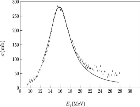
Figure 15: Giant resonance in the absorption of photons by ¹²⁰Sn [Le74].

Figure 15 exhibits the excitation function of photoabsorption of ¹²⁰Sn around the electric dipole giant resonance at 15 MeV. The giant resonance happens in nuclei along the whole periodic table, with the resonance energy decreasing with $A$ without large oscillations (see Figure 16) starting at $A=20$. This shows that the giant resonance is a property of the nuclear matter and not a characteristic phenomenon of nuclei of a certain type. The widths of the resonances are almost all in the range between 3.5 MeV and 5 MeV. It can reach 7 MeV in a few cases.

In the Goldhaber-Teller model [GT48], the photon, through the action of its electric field on the protons, takes the nucleus to an excited state where a group of protons oscillates in opposite phase against a group of neutrons. In such an oscillation, those groups interpenetrate, keeping constant the incompressibility of each group separately. A classic calculation using this hypothesis leads to a vibration frequency that varies with the inverse of the squared root of the nuclear radius, i.e., the resonance energy varies with $A^{-1/6}$.

In the Steinwedel-Jensen model [SJ50] developed a classic study of the oscillation in another way, already suggested by Goldhaber and Teller, in which the incompressibility is abandoned. The nucleons move inside of a fixed spherical cavity with the proton and neutron densities being a function of the position and time. The nucleons at the surface have fixed position with respect to each other and the density is written in such a way that, at a given instant, the excess of protons on one side of the nucleus coincides with the lack of neutrons on that same side, and vice-versa. Such a model leads to a variation of the resonance energy with $A^{-1/3}$.

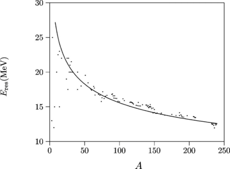
Figure 16: Location of the energy of the giant electric dipole resonance given by (185) (continuous curve), compared with experimental points [DB88].

If one assumes a mixed contribution of the two models, obtains an expression for $E_{GDR}$ as function of the mass number $A$ [Mye77],

$$E_{GDR}(\text{MeV})=112\times\left[A^{2/3}+(A_{0}A)^{1/3}\right]^{-1/2},$$ (185)

where $A_{0}\cong 274$. This expression, with the exception of some very light nuclei, reproduces the behavior of the experimental values very well, as we can see in Figure 16. An examination of Equation (185) shows that the Gamow-Teller mode prevails broadly in light nuclei, while the contribution of the Steinwedel-Jensen mode is negligible. The latter mode increases with $A$ but it only becomes predominant at the end of the periodic table, at $A=A_{0}$.

The giant electric dipole resonance arises from an excitation that transmits 1 unit of angular momentum to the nucleus ($\Delta l=1$). If the nucleus is even-even it is taken to a $1^{-}$ state. What one verifies is that the transition also changes the isospin of 1 unit ($\Delta T=1$) and, due to that, it is also named an isovector resonance. Giant isoscalar resonances ($\Delta T=0$) of electric quadrupole ($\Delta l=2$) [PW71] and electric monopole ($\Delta l=0$) [Ma75] were observed in reactions with charged particles. The first is similar to the vibrational quadrupole state created by the absorption of a phonon of $\lambda=2$, since both are, in even-even nuclei, states of $2^{+}$ vibration. But the giant quadrupole resonance has a much larger energy. This resonance energy, in the same way argued for the dipole, decreases smoothly with $A$, obeying the approximate formula

$${E_{GQR}(}\text{{MeV}}{)\cong 62A^{-1/3}.}$$ (186)

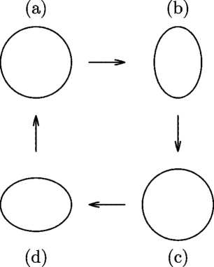
Figure 17: Four stages in the vibration cycle of a giant quadrupole resonance. In an isoscalar resonance, protons and neutrons vibrate in phase, while in an isovector resonance, the vibrations occur in opposite phase. For opposite phases, when the protons are at the stage (b), the neutrons will be at the stage (d), and vice-versa.

In the state of giant electric quadrupole resonance the nucleus oscillates between the spherical (supposing that this is the form of the ground state) and ellipsoidal form. If protons and neutrons act in phase, we have an isoscalar resonance ($\Delta T=0$) and if they oscillate in opposite phase the resonance is isovector ($\Delta T=1$). Figure 17 illustrates these two possible vibration modes.

The giant monopole resonance is a very special way of nuclear excitation where the nucleus contracts and expands radially, maintaining its original form but changing its volume. It is also called the breathing mode. It can also happen in the isoscalar and isovector forms. It is an important way to study the compressibility of nuclear matter. Again here, the isoscalar form has a reasonable number of measured cases, the location of the resonance energy being given by the approximate expression

$$E_{GMR}(\text{MeV})\cong 80A^{-1/3}.$$ (187)

Besides the electric giant resonances, associated to a variation in the form of the nucleus, magnetic giant resonances exist, involving what one calls by spin vibrations. In these, nucleons with spin upward move out of phase with nucleons with spin downward. The number of nucleons involved in the process cannot be very large because it is limited by the Pauli principle.

Another important aspect of the study of the giant resonances is the possibility that they can be induced in already excited nuclei. This possibility was analyzed theoretically by D. M. Brink and P. Axel [Ax62] for giant resonances excited “on top” of nuclei rotating with high angular momentum, resulting in the suggestion that the frequency and other properties of the giant resonances are not affected by the excitation. A series of experiences in the decade of the 1980’s (see Reference [BB86a]) gave support to this hypothesis.

A special case happens when the giant resonance is excited on top of another giant resonance. Understanding the excitation of a giant resonance as the result of the absorption of one phonon, we can view these double giant resonances as states of excitation with two vibrational phonons. The double giant dipole resonance was observed for the first time in reactions with double charge exchange induced by pions in ³²S [Mo88]. As first shown in reference [BB86] a much better possibility to study multiple giant resonances is by means of Coulomb excitation with relativistic heavy projectiles. Later on, this was indeed verified experimentally and several properties of multiple giant resonances have been studied theoretically (for a theoretical review, see [BP99]).

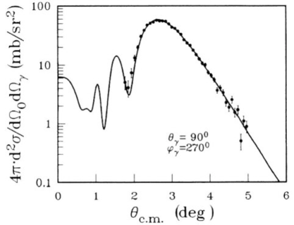
Figure 18: Cross section for the excitation of the giant dipole resonance followed by $\gamma$-decay to the ground state in the reaction ²⁰⁸Pb(¹⁷O,¹⁷O’$\gamma_{0}$) at 84 MeV/nucleon for fixed $\gamma$ angle $\theta_{\gamma}=90^{\mathrm{o}}$ and $\phi_{\gamma}=270^{\mathrm{o}}$. The points are experimental [Bee90]. The curve is predicted for Coulomb excitation.

Figure 18 shows the cross section for the excitation of the giant dipole resonance followed by $\gamma$-decay to the ground state in the reaction ²⁰⁸Pb(¹⁷O,¹⁷O’$\gamma_{0}$) at 84 MeV/nucleon for fixed $\gamma$ angle $\theta_{\gamma}=90^{\mathrm{o}}$ and $\phi_{\gamma}=270^{\mathrm{o}}$. The points are experimental [Bee90]. The curve is predicted for Coulomb excitation using the eikonal wavefunction, as described in the previous section, and a reduced transition strength calculated according the deformed potential model [BN93]. The agreement with the data is excellent.

VII.2 Sum Rules

It is useful to be able to estimate the total photoabsorption cross section summed over all transitions $|i\rangle\rightarrow|f\rangle$ from the initial, for instance ground, state. Such estimates are given by the sum rules (SR) which approximately determine quantities of the following type:

$${\cal S}^{(n)}_{i}[F]=\frac{1}{2}\sum_{f}(E_{f}-E_{i})^{n}\Bigl{\{}\Bigl{|}\langle f|F|i\rangle\Bigr{|}^{2}+\Bigl{|}\langle f|F^{\dagger}|i\rangle\Bigr{|}^{2}\Bigr{\}}.$$ (188)

Here the transition probabilities for an arbitrary pair of mutually conjugate operators $F$ and $F^{\dagger}$ are weighted with a certain (positive, negative or equal to zero) power $n$ of the transition energy. For a hermitian operator $F=F^{\dagger}$ the two terms in (188) are equal and the factor 1/2 is cancelled.

The exact result follows immediately for non-energy-weighted SR, $n=0$, based on the completeness of the set of the states $|f\rangle$,

$${\cal S}^{(0)}_{i}[F]=\frac{1}{2}\langle i|F^{\dagger}F+FF^{\dagger}|i\rangle.$$ (189)

Often it turns out to be possible to get a good estimate for the expectation value in the right hand side of (189), or to extract it from data.

For the energy-weighted sum rules (EWSR), ${\cal S}^{(1)}$, a reasonable estimate can be derived for many operators under certain assumptions about the interactions in the system. First, using again the completeness of the intermediate states $|f\rangle$, we can identically write down ${\cal S}^{(1)}$ as an expectation value in the initial state $|i\rangle$ of the double commutator

$${\cal S}^{(1)}_{i}[F]=\frac{1}{2}\langle i|\Bigl{[}[F,H],F^{\dagger}\Bigr{]}|i\rangle,$$ (190)

where $H$ is the total hamiltonian which has energies $E_{i}$ and $E_{f}$ as its eigenvalues. Thus, we again need to know the properties of the initial state only. Now we choose the operator $F$ as a one-body quantity depending on coordinates ${\bf r}_{a}$ of the particles,

$$F=\sum_{a}f_{a},\quad f_{a}=f({\bf r}_{a}).$$ (191)

Apart from that we assume that the hamiltonian does not contain momentum-dependent interactions. Then only the kinetic part of the hamiltonian contributes to $[F,H]$, and the result can be found explicitly,

$$[F,H]=\Bigl{[}\sum_{a}f_{a},\sum_{b}\frac{{\bf p}_{b}^{2}}{2m_{b}}\Bigr{]}=\sum_{a}\frac{i\hbar}{2m_{a}}[(\nabla_{a}f_{a}),{\bf p}_{a}]_{+},$$ (192)

where $[...\,,\,...]_{+}$ denotes the anticommutator. The outer commutator in (190) leads now to the simple result

$${\cal S}^{(1)}_{i}[F]=\sum_{a}\frac{\hbar^{2}}{2m_{a}}\langle i|\Bigl{|}\nabla_{a}f_{a}\Bigr{|}^{2}|i\rangle.$$ (193)

As an example we take the charge form factor

$$F=\sum_{a}e_{a}e^{i({\bf k}\cdot{\bf r}_{a})}.$$ (194)

The sum rule in this case is universal for any initial state $|i\rangle$,

$${\cal S}^{(1)}[F]=\hbar^{2}{\bf k}^{2}\sum_{a}\frac{e_{a}^{2}}{2m_{a}}.$$ (195)

Taking ${\bf k}$ along an (arbitrary) $z$-axis and considering the long wavelength limit, $kR\ll 1$, we get from the first nonvanishing term in the expansion of the exponent the EWSR for the dipole operator, $d_{z}=rY_{10}(\hat{\bf r})$,

$${\cal S}^{(1)}[d_{z}]=\sum_{a}\frac{\hbar^{2}e_{a}^{2}}{2m_{a}}.$$ (196)

This is an extension of the old Thomas-Reiche-Kuhn (TRK) dipole SR in atomic physics. For a neutral atom, in the center-of-mass frame attached to the nucleus of charge $Z$ (here $m$ is the electron mass),

$$S^{(1)}[d_{z}]=\frac{\hbar^{2}e^{2}}{2m}Z.$$ (197)

The atomic TRK SR is essentially exact (up to relativistic velocity-dependent corrections).

In (194) $e_{a}$ are in fact arbitrary numbers. For intrinsic dipole excitations we have to exclude the center-of-mass motion. Therefore our $z$-coordinates should be intrinsic coordinates, $z_{a}\Rightarrow z_{a}-R_{z}$, where $R_{z}=\sum_{a}z_{a}/A$. Hence, the intrinsic dipole moment is

$$d_{z}=\sum_{a}e_{a}(z_{a}-R_{z})=e\sum_{p}z_{p}-\frac{Ze}{A}\Bigl{(}\sum_{p}z_{p}+\sum_{n}z_{n}\Bigr{)}.$$ (198)

This operator can be rewritten as

$$d_{z}=e_{p}\sum_{p}z_{p}+e_{n}\sum_{n}z_{n}$$ (199)

where protons and neutrons carry effective charges

$$e_{p}=\frac{N}{A}e,\quad e_{n}=-\frac{Z}{A}e.$$ (200)

Now (196) gives the dipole EWSR

$${\cal S}^{(1)}_{i}[d_{z}] \equiv \sum_{f}E_{fi}|d^{z}_{fi}|^{2}$$ (201)

$$= \frac{\hbar^{2}e^{2}}{2m_{N}}\left[Z\left(\frac{N}{A}\right)^{2}+N\left(\frac{-Z}{A}\right)^{2}\right]$$ (202)

$$= \frac{\hbar^{2}e^{2}}{2m_{N}}\frac{NZ}{A},$$ (203)

where $m_{N}$ is the nucleon mass.

The factor $(NZ/A)$ is connected to the reduced mass for relative motion of neutrons against protons as required at the fixed center of mass. This result does not include the dipole strength related to nuclear motion as a whole. According to the classical SR (197), this contribution is $(m\rightarrow Am_{N},\,e\rightarrow Ze)$

$${\cal S}^{(1)}[{\rm c.m.}]=\frac{\hbar^{2}(Ze)^{2}}{2Am_{N}}.$$ (204)

The sum of the global (204) and intrinsic (203) dipole strength recovers the full TRK SR (197),

$${\cal S}^{(1)}_{i}[{\rm tot.\;dip}]=\frac{\hbar^{2}e^{2}}{2m_{N}}\left(\frac{NZ}{A}+\frac{Z^{2}}{A}\right)=\frac{\hbar^{2}e^{2}}{2m_{N}}Z.$$ (205)

In contrast to the atomic TRK case, the nuclear dipole EWSR (203) cannot be exact. Velocity-dependent and exchange forces are certainly present in nuclear interactions. Nevertheless, Eq. (203) gives a surprisingly good estimate of the realistic dipole strength which is not fully understood. In a similar way one can consider SR for other multipoles but the results are not universal and in general depend on the initial state.

The EWSR (203) is what we need to evaluate the sum of integral dipole cross sections for real photons over all possible final states $|f\rangle$. Taking the photon polarization vector along the $z$-axis, we come to the total dipole photoabsorption cross section

$$\sigma_{tot}^{\gamma}=\sum_{f}\int dE_{\gamma}\sigma_{fi}^{\gamma}=2\pi^{2}\frac{e^{2}\hbar}{m_{N}c}\frac{ZN}{A}.$$ (206)

This universal prediction,

$$\sigma_{tot}^{\gamma}=0.06\frac{ZN}{A}{\rm barn}\cdot{\rm MeV},$$ (207)

on average agrees well with experiments in spite of crudeness of approximations made in the derivation. One should remember that it includes only dipole absorption.

For the E2 isoscalar giant quadrupole resonances one has the approximate sum rule [BM75]

$$\int{dE_{\gamma}\over E_{\gamma}^{2}}\sigma_{GQR}^{\gamma}(E_{\gamma})\simeq 0.22ZA^{2/3}\ \mu{\rm b\ MeV}^{-1}.$$ (208)

VII.3 Coulomb excitation of giant resonances

A simple estimate of Coulomb excitation of giant resonances based on sum rules can be made by assuming that the virtual photon numbers vary slowly compared to the photonuclear cross sections around the resonance peak. Then

$$\sigma_{C} \simeq {N_{E1}(E_{GDR})\over E_{GDR}}\int dE_{\gamma}\sigma_{GDR}^{\gamma}(E_{\gamma})$$ (209)

$$+ N_{E2}(E_{GQR})E_{GQR}\int{dE_{\gamma}\over E_{\gamma}^{2}}\sigma_{GQR}^{\gamma}(E_{\gamma}).$$

In figure 19 we show the Coulomb excitation cross section of giant resonances in ⁴⁰Ca projectiles hitting a ²³⁸U target as a function of the laboratory energy per nucleon. The dashed line corresponds to the excitation of the giant electric dipole resonance, the dotted to the electric quadrupole, and the lower line to the magnetic dipole which was also obtained using a sum-rule for M1 excitations [BB88]. The solid curve is the sum of these contributions.

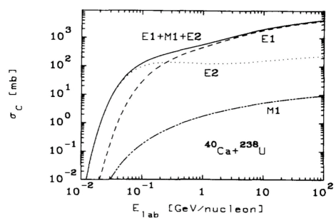
Figure 19: Coulomb excitation cross section of giant resonances in ⁴⁰Ca projectiles hitting a ²³⁸U target as a function of the laboratory energy per nucleon. The dashed line corresponds to the excitation of the giant electric dipole resonance, the dotted to the electric quadrupole, and the lower line to the magnetic dipole. The solid curve is the sum of these contributions.

The cross sections increase very rapidly to large values, which are already attained at intermediate energies. A salient feature is that the cross section for the excitation of giant quadrupole modes is very large at low and intermediate energies, decreasing in importance (about $10$% of the $E1$ cross section) as the energy increases above 1 GeV/nucleon. This occurs because the equivalent photon number for the $E2$ multipolarity is much larger than that for the $E1$ multipolarity at low collision energies. That is, $n_{E2}\gg n_{E1}$, for $v\ll c$. This has a simple explanation, as we already discussed in connection with figure 11. Pictorially, as seen from an observator at rest, when a charged particle moves at low energies the lines of force of its corresponding electric field are isotropic, diverging from its center in all directions. This means that the field carries a large amount of tidal ($E2$) components. On the other hand, when the particle moves very fast its lines of force appear contracted in the direction perpendicular to its motion due to Lorentz contraction. For the observator this field looks like a pulse of plane waves of light. But plane waves contain all multipolarities with the same weight, and the equivalent photon numbers become all approximately equal, i.e., $n_{E1}\simeq n_{E2}\simeq n_{M1}$, and increase logarithmically with the energy for $\gamma\gg 1$. The difference in the cross sections when $\gamma\gg 1$ are then approximately equal to the difference in the relative strength of the two giant resonances $\sigma_{\gamma}^{E2}/\sigma^{E1}_{\gamma}<0.1$. The excitation of giant magnetic monopole resonances is of less importance, since for low energies $n_{M1}\ll n_{E1}$ ($n_{M1}\simeq(v/c)^{2}n_{E1}$), whereas for high energies, where $n_{M1}\simeq n_{E1}$, it will be also much smaller than the excitation of electric dipole resonances since their relative strength $\sigma^{M1}_{\gamma}/\sigma^{E1}_{\gamma}$ is much smaller than unity.

At very large energies the cross sections for the Coulomb excitation of giant resonances overcome the nuclear geometrical cross sections. Since these resonances decay mostly through particle emission or fission, this indicates that Coulomb excitation of giant resonances is a very important process to be considered in relativistic heavy ion collisions and fragmentation processes, especially in heavy ion colliders. At intermediate energies the cross sections are also large and this offers good possibilities to establish and study the properties of giant resonances.

The formalism described in the previous sections has also been used in the analysis of the data of Ref. [BB90], in which a projectile of ¹⁷O with an energy of $E_{lab}=84$ MeV/nucleon excites the target nucleus ²⁰⁸Pb to the Giant Dipole Resonance (GDR). The optical potential has a standard Woods-Saxon form with parameters given in Ref. [BB90]. In order to calculate the inelastic cross section for the excitation of the GDR, one can use a Lorentzian parameterization for the photoabsorption cross section of ²⁰⁸Pb [Ve70],

$$\sigma_{\pi\lambda}^{\gamma}=\sigma_{m}\;{E_{\gamma}^{2}\Gamma^{2}\over(E_{\gamma}^{2}-E_{R}^{2})^{2}+E_{\gamma}^{2}\Gamma^{2}}.$$ (210)

with $\sigma_{m}$ chosen to reproduce the Thomas-Reiche-Kuhn sum rule for $E1$ excitations, and Eq. (208) for isoscalar giant quadrupole resonances. We use the widths $\Gamma_{\mbox{\tiny GDR}}=4\;$MeV and $\Gamma_{\mbox{\tiny GQR}}=2.2\;$MeV for ²⁰⁸Pb.

At $\sim 84$ MeV/nucleon the maximum scattering angle which still leads to a pure Coulomb scattering (assuming a sharp cut-off at an impact parameter $b=R_{P}+R_{T}$) is $\sim 4^{\circ}$. Inserting this form into Eq. (164) and doing the calculations implicit in Eq. (162) for $dn_{E1}/d\Omega$, one obtains the angular distribution which is compared to the data in Fig. 21. The agreement with the data is excellent, provided one adjusts the overall normalization to a value corresponding to $93\,\%$ of the energy weighted sum rule (EWSR) in the energy interval $7-18.9\;$MeV (see section 6.10). Taking into account the $\pm 10\%$ uncertainty in the absolute cross sections quoted in Ref.  [Bar88], this is consistent with photoabsorption cross section in that energy range.

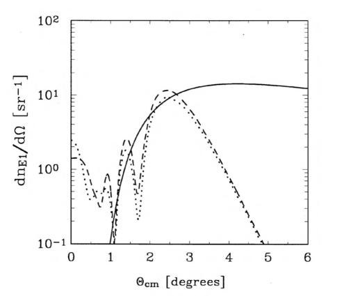
Figure 20: Virtual photon numbers for the electric dipole multipolarity generated by 84A MeV ¹⁷O projectiles incident on ²⁰⁸Pb, as a function of the center-of-mass scattering angle. The solid curve is a semiclassical calculation. The dashed and dotted curves are eikonal calculations with and without relativistic corrections, respectively.

To unravel the effects of relativistic corrections, one  can repeat the previous calculations unplugging the factor $\gamma=(1-v^{2}/c^{2})^{-1}$ which appears in the expressions (165) and (166) and using the non-relativistic limit of the functions $G_{E1m}$ of Eq. (V.1). These modifications eliminate the relativistic corrections on the interaction potential. The result of this calculation is shown in fig. 20 (dotted curve). For comparison, the result of a full calculation, keeping the relativistic corrections (dashed curve), is also shown. One observes that the two results have approximately the same pattern, except that the non-relativistic result is slightly smaller than the relativistic one. In fact, if one repeats the calculation for the excitation of GDR using the non-relativistic limit of eqs. (165) and (166), one finds that the best fit to the data is obtained by exhausting $113\,\%$ of the EWSR. This value is very close to the $110\,\%$ obtained in Ref. [Bar88].

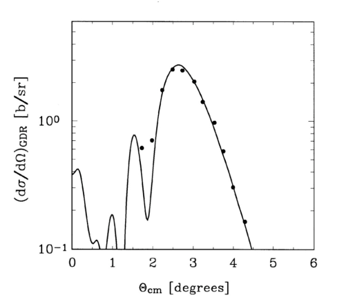
Figure 21: Differential cross section for the excitation of the isovector giant dipole resonance in ²⁰⁸Pb by means of ¹⁷0 projectiles at 84 MeV/nucleon, as a function of the center-of-mass scattering angle. Data are from Ref. [BB90]. The theoretical calculation is from Ref. [BN93].

In fig. 20 we also show the result of a semiclassical calculation (solid curve) for the GDR excitation in lead, using Eq.  (179) for the virtual photon numbers. The semiclassical curve is not able to fit the experimental data in figure 21, which shows a perfect agreement with the Coulomb excitation with the eikonal approximation [BN93]. This is mainly because diffraction effects and strong absorption are not included. But the semiclassical calculation displays the region of relevance for Coulomb excitation. At small angles the scattering is dominated by large impact parameters, for which the Coulomb field is weak. Therefore the Coulomb excitation is small and the semiclassical approximation fails. It also fails in describing the large angle data (dark-side of the rainbow angle), since absorption is not treated properly. One sees that there is a “window” in the inelastic scattering data near $\theta=2-3^{\circ}$ in which the semiclassical and full calculations give approximately the same cross section.

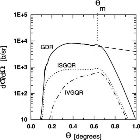
Figure 22: Differential cross section for the excitation of a giant dipole resonance in Pb+Pb collisions at 640 MeV/nucleon, as a function of the center of mass scattering angle.

In fig. 22 we show a similar calculation, but for the excitation of the GDR in Pb for the collision ²⁰⁸Pb + ²⁰⁸Pb at 640 MeV/nucleon. The dashed line is the result of a semiclassical calculation. Here we see that a purely semiclassical calculation, is able to reproduce the quantum results up to a maximum scattering angle $\theta_{m}$, at which strong absorption sets in. This justifies the use of semiclassical calculations for heavy systems, even to calculate angular distributions. The cross sections increase rapidly with increasing scattering angle, up to an approximately constant value as the maximum Coulomb scattering angle is approached. This is explained as follows. Very forward angles correspond to large impact parameter collisions in which case $\omega b/\gamma v>1$, the virtual photon numbers in Eq. (165) drop quickly to zero, and the excitation of giant resonances in the nuclei is not achieved. As the impact parameter decreases, increasing the scattering angle, $\omega b/\gamma v\lesssim 1$ and excitation occurs.

VII.4 Excitation and photon decay of the GDR

We now consider the excitation of the target nucleus to the giant dipole resonance and the subsequent photon decay of that excited nucleus, leaving the target in the ground state. Experimentally, one detects the inelastically scattered projectile in coincidence with the decay photon and demands that the energy lost by the projectile is equal to the energy of the detected photon. To the extent that the excitation mechanism is dominated by Coulomb excitation, with the exchange of a single virtual photon, this reaction is very similar to the photon scattering reaction, except that in the present case the incident photon is virtual rather than real. In this section, we investigate whether the connection between these two reactions can be formalized.

We have seen that, under the conditions $\Delta E/E\ll 1$, the cross section for excitation of the target nucleus factorizes into the following expression (we assume that the contribution of the $E1$-multipolarity is dominant):

$${\frac{d^{2}\sigma_{C}}{d\Omega dE_{\gamma}}}\left(E_{\gamma}\right)={\frac{1}{E_{\gamma}}}\ {\frac{dn_{\gamma}}{d\Omega}}\left(E_{\gamma}\right)\ \sigma_{\gamma}\left(E_{\gamma}\right).$$ (211)

Figure 23 the cross section for the excitation of the GDR without the detection of the decay photon. Data are from Ref.  [Bee90]. The solid line is a calculation from Ref. [BN93] using the eikonal wavefunction for the Coulomb excitation.

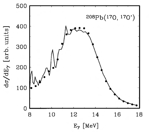
Figure 23: Cross section for the excitation of the GDR without the detection of the decay photon. Data are from Ref.  [Bee90]. The solid line is a calculation from Ref. [BN93].

The usual way to write the cross section $d^{2}\sigma_{C\gamma}/d\Omega dE_{\gamma}$ for the excitation of the target followed by photon decay to the ground state is simply to multiply the above expression by a branching ratio $R_{\gamma}$, which represents the probability that the nucleus excited to an energy $E_{\gamma}$ will emit a photon leaving it in the ground state [Bee90]:

$${\frac{d^{2}\sigma_{C\gamma}}{d\Omega dE_{\gamma}}}\left(E_{\gamma}\right)={\frac{1}{E_{\gamma}}}\ {\frac{dn_{\gamma}}{d\Omega}}\left(E_{\gamma}\right)\ \sigma_{\gamma}\left(E_{\gamma}\right)\ R_{\gamma}\left(E_{\gamma}\right).$$ (212)

Instead, one can also use the following expression, in complete analogy with Eq.  (211):

$${\frac{d^{2}\sigma_{C\gamma}}{d\Omega dE_{\gamma}}}\left(E_{\gamma}\right)={\frac{1}{E_{\gamma}}}\ {\frac{dn_{\gamma}}{d\Omega}}\left(E_{\gamma}\right)\ \sigma_{\gamma\gamma}\left(E_{\gamma}\right),$$ (213)

where $\sigma_{\gamma\gamma}\left(E_{\gamma}\right)$ is the cross section for the elastic scattering of photons with energy $E_{\gamma}$. Formally, these expressions are equivalent in that they simply define the quantity $R_{\gamma}$. However, if one treats $R_{\gamma}$ literally as a branching ratio, then these expressions are equivalent only if it were true that the photon scattering cross section is just product of the photoabsorption cross section and the branching ratio. In fact, it is well-known from the theory of photon scattering that the relationship between the photoabsorption cross section and the photon scattering cross section is more complicated. In particular, it is not correct to think of photon scattering as a two-step process consisting of absorption, in which the target nucleus is excited to an intermediate state of energy $E_{\gamma}$, followed by emission, in which the emitted photon has the same energy $E_{\gamma}$. Since the intermediate state is not observable, one must sum over all possible intermediate states and not just those allowed by conservation of energy. Now, if the energy $E_{\gamma}$ happens to coincide with a narrow level, then that level will completely dominate in the sum over intermediate states. In that case, it is proper to regard the scattering as a two-step process in the manner described above, and the two expressions for the cross section will be equal. However, for $E_{\gamma}$ in the nuclear continuum region (e.g., in the region of the GDR), this will not be the case.

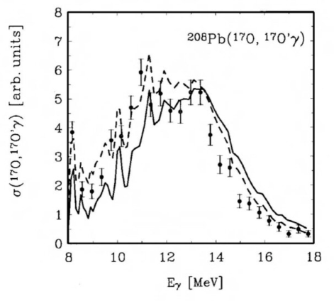
Figure 24: Cross section for excitation followed by $\gamma$-decay of ²⁰⁸Pb by ¹⁷O projectiles at 84A MeV. The solid (dashed) line includes (excludes) the Thompson scattering amplitude. Data are from Ref.   [Bee90].

The calculation [BN93] is compared to the data in fig. 24. The left part shows the cross section for the excitation of the GDR without the detection of the decay photon. The agreement with the data is excellent. The right part of fig. 24 shows the cross section for the excitation-decay process as a function of $E_{\gamma}$. Although the qualitative trend of the data are well described, the calculation systematically overpredicts the cross section on the high-energy side of the GDR (solid curve). If the Thompson amplitude is not included in $\sigma_{\gamma\gamma}$, the calculation is in significantly better agreement with the data (dashed curve).

VII.5 Multiphonon resonances

The Coulomb excitation of harmonic vibrations is formulated in Appendix F. The formalism can be applied to excitation of multiple giant resonances, i.e. giant resonances excited on top of other giant resonances, also called multiphonon giant resonances. Coulomb excitation of multiphonon giant resonances was formulated in the harmonic vibrator model in Ref. [BB86]. The excitation of multiphonon states may be viewed as the absorption by the target (projectile) of several photons from the pulse of equivalent photons generated by the relativistic projectile (target); or it can be also described as multiple excitation of a harmonic oscillator with GDR quantum energy.

As explained in Appendix F, the probability for the excitation of a $N$-phonon state, $P_{N}(b)$ can be obtained from the first-order theory for the probability, $P_{f.o.}(b)$,

$$P_{N}=\frac{1}{N!}\;\left|P_{1st}(b)\right|^{N}\;\exp\left[-P_{1st}(b)\right].$$ (214)

$P_{1st}(b)$ is calculated as in explained in the previous sections.

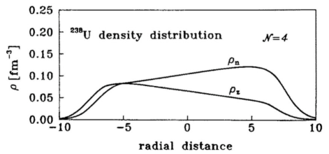
Figure 25: Proton and neutron density distributions at the moment of largest separation between them in a $N=4$ multiphonon state in ²³⁸U [VGB90].

The multiphonon states correspond to large-amplitude vibrations of neutrons against protons in nuclei. Although the energy deposit is small (multiples of the energy of a GDR state), such large collective motion may lead to exotic decays of the nuclei. This is a relatively cold fragmentation process, in contrast to the violent fragmentation following central collisions of relativistic heavy ion collisions, in which high pressures and temperatures are achieved. Figure 25 shows the neutron and proton matter distribution in ²³⁸U for a $N=4$ multiphonon GDR state at the moment of maximum displacement [VGB90].

The first Coulomb excitation experiments for the excitation of the double giant dipole resonance (DGDR) were performed at the GSI facility in Darmstadt/Germany [Rit93,Sch93]. In Fig. 26 we show the result of one of these experiments [Sch93], which looked for the neutron decay channels of giant resonances excited in relativistic projectiles. The excitation spectrum of relativistic ¹³⁶Xe projectiles incident on Pb are compared with the spectrum obtained in C targets. A comparison of the two spectra immediately proofs that nuclear contribution to the excitation is very small. Another experiment [Rit93] dealt with the photon decay of the double giant resonance. A clear bump in the spectra of coincident photon pairs was observed around the energy of two times the GDR centroid energy in ²⁰⁸Pb targets excited with relativistic ²⁰⁹Bi projectiles.

Figure 26: Experimental results for ¹³⁶Xe projectile excitation (at 690 MeV/nucleon) on a Pb target (squares) and a C target (circles). The spectrum for the C target is multiplied by a factor 2 for better presentation. The resonance energies for one and two-phonon giant resonances are indicated. The dashed curve reflects the results of a first-order calculation for the Pb target. The figure is taken from Ref. [Sch93].

Much of the interest on multiphonon resonances relies on the possibility of looking at exotic particle decay of these states. Since there is more energy deposit in the nuclei, other decay channels are open for the multiphonon states. Generally, the GRs in heavy nuclei decay by neutron emission. One expects that the double, or triple, GDR decays mainly in the 2n and 3n decay channel. In fact, such a picture has been adopted in [ABS93] with success to explain the total cross sections for the neutron removal in peripheral collisions.

Coulomb excitation of multiphonon resonances is a rich playground for theories of nuclear response. There are still open issues related to the magnitude of the cross sections, the widths of the multiphonon states and the excitation mechanisms in general. Some of the reviews on the subject are Refs. [ABE98,BP99].

VIII Intermediate energy collisions

The semiclassical theory of Coulomb excitation in low energy collisions accounts for the Rutherford bending of the trajectory, but relativistic retardation effects are neglected [AW75]. On the other hand, in the theory of relativistic Coulomb excitation [WA79] recoil effects on the trajectory are neglected (one assumes straight-line motion) but retardation is handled correctly. In fact, the onset of retardation brings new important effects such as the steady increase of the excitation cross sections with bombarding energy. In a heavy ion collision around 100A MeV the Lorentz factor $\gamma$ is about 1.1. Since this factor enters the excitation cross sections in many ways, such as in the adiabacity parameter, $\xi(R)={\omega_{fi}R/}\gamma v$, one expects that some sizable modifications in the theory of relativistic Coulomb excitation should occur [AB89]. Recoil corrections are not negligible either, and the relativistic calculations based on the straight-line parametrization should not be completely appropriate to describe the excitation probabilities and cross sections. The Coulomb recoil in a single collision is of the order of $a_{0}={{Z_{1}Z_{2}e^{2}}/{m_{0}v^{2}},}$ which is half-distance of closest approach in a head-on collision, with m₀ equal to the reduced mass of the colliding nuclei. Although this recoil is small for intermediate energy collisions, the excitation probabilities are quite sensitive to it. This is important for example in the excitation of giant resonances because the adiabacity parameter is of the order of one. When $\xi(b)\ll 1$, the excitation probabilities depends on $b$ approximately like $1/b^{2}$, while when $\xi(b)$ becomes greater than one they decrease approximately as $e^{-2\pi\xi(b)}/b^{2}$. Therefore, when $\xi\simeq 1$ a slight change of $b$ may vary appreciably the excitation probabilities.

VIII.1 Recoil and retardation corrections

In intermediate energy collisions, where one wants to account for recoil and retardation simultaneously, one should solve the general classical problem of the motion of two relativistic charged particles. This has been studied in Refs. [AB89,AAB90]. But, even if radiation is neglected, this problem can only be solved if one particle has infinite mass [LL79]. This approximation should be sufficient if we take, e.g., the collision ¹⁶O + ²⁰⁸Pb as our system.

In the classical one-body problem, one starts with the relativistic Lagrangian

$$\mathcal{L}=-m_{o}c^{2}\left\{1-{\frac{1}{c^{2}}}\,({\dot{r}}^{2}+r^{2}{\dot{\phi}}^{2})\right\}^{1/2}-{\frac{Z_{1}Z_{2}e^{2}}{r}}\ ,$$ (215)

where ${\dot{r}}$ and ${\dot{\phi}}$ are the radial and the angular velocity of the particle, respectively. Using the Euler-Lagrange equations one finds three kinds of solutions, depending on the sign of the charges and the angular momentum in the collision. In the case of our interest, the appropriate solution relating the collisional angle $\phi$ and the distance r between the nuclei is [LL79]

$${\frac{1}{r}}=A\left[\epsilon\;\cos(W\phi)-1\right]$$ (216)

where

$$W = \left[1-({\frac{Z_{1}Z_{2}e^{2}}{c{L}_{0}}})^{2}\right]^{1/2},\;\;\;\;\;\;A={\frac{Z_{1}Z_{2}e^{2}E}{c^{2}{L}_{0}^{2}W^{2}}}\,,$$ (217)

$$\epsilon = {\frac{c{L}_{0}}{Z_{1}Z_{2}e^{2}E}}\,\left[E^{2}-m_{0}^{2}c^{4}+({\frac{m_{0}cZ_{1}Z_{2}e^{2}}{{L}_{0}}})^{2}\right]^{1/2}\,.$$ (218)

$E$ is the total bombarding energy in MeV, $m_{0}$ is the mass of the particle and ${L}_{0}$ its angular momentum. In terms of the Lorentz factor $\gamma$ and of the impact parameter $b$, $E=\gamma m_{o}c^{2}$ and ${L}_{0}=\gamma m_{0}vb$. The above solution is valid if ${L}_{0}>Z_{1}Z_{2}e^{2}/c$. In heavy ion collisions at intermediate energies one has $L_{0}\gg Z_{1}Z_{2}e^{2}/c$ for impact parameters that do not lead to strong interactions. It is also easy to show that, from the magnitudes of the parameters involved in heavy ion collisions at intermediate energies, the trajectory (216) can be very well described by approximating

$$W=1\,,\qquad A=\frac{a_{0}}{\gamma b^{2}}\,,\qquad\epsilon=\sqrt{{\frac{b^{2}\gamma^{2}}{a_{0}^{2}}}+1}\ ,$$ (219)

where $a_{0}$ is half the distance of closest approach in a head on collision (if the nuclei were pointlike and if non-relativistic kinematics were used), and $\epsilon$ is the eccentricity parameter. In the approximation (219) $\epsilon$ is related to the deflection angle $\vartheta$ by $\epsilon=(a_{0}/\gamma)\cot\vartheta$.

The time dependence for a particle moving along the trajectory, Eq. (216), may be directly obtained by solving the equation of angular momentum conservation. Introducing the parametrization

$$r(\chi)={\frac{a_{0}}{\gamma}}\,\left[\epsilon\,\cosh\chi+1\right]$$ (220)

we find

$$t={\frac{a_{0}}{\gamma v}}\,\left[\chi+\epsilon\,\sinh\chi\right]\,.$$ (221)

Using the scattering plane perpendicular to the z-axis, one finds that the corresponding components of $\mathbf{r}$ may be written as

$$x = a\,\left[\cosh\chi+\epsilon\right]\ ,$$

$$y = a\,\sqrt{\epsilon^{2}-1}\,\sinh\chi\ ,$$

$$z = 0\ ,$$ (222)

where $a=a_{0}/\gamma$. This parametrization is of the same form as in the non-relativistic case, Eq. (85), except that $a_{0}$ replaced by $a_{0}/\gamma\equiv a$.

Non-relativistically the two-body problem is solvable by introduction of center of mass and relative motion coordinates. Then, the result is equivalent to that of a particle with reduced mass $m_{0}=m_{P}m_{T}/(m_{P}+m_{T})$ under the action of the same potential. The particle with reduced mass m₀ is lighter than those with mass m_P and m_T, and this accounts for the simultaneous recoil of them. An exact relativistic solution should reproduce this behavior as the relative motion energy is lowered. We can use the reduced mass definition of m₀ as usual in the parametrization of the classical trajectory of Coulomb excitation in intermediate energy collisions, as outlined above. For a ¹⁶O + ²⁰⁸Pb collision this is not a bad approximation. For heavier systems like U+U it would be the simplest way to overcome this difficulty. But, as energy increases, this approximation is again unimportant since the trajectories will be straight-lines parametrized by an impact parameter b. An exact result was obtained numerically in Ref. [AAB90] using the Darwin Lagrangian to determine the classical trajectory in collisions at intermediate energies. But, the parametrization of the classical trajectory as given by Eqs. (222) with a reduced mass particle, besides reproducing both the non-relativistic and the relativistic energies, gives a reasonable solution to the kind of collisions we want to study.

From here on the procedure is the same as in the derivation of low-energy excitation amplitudes. Whenever $a_{0}$ appears in those equations it will have to be replaced by $a_{0}/\gamma$. The orbital integrals in Eqs. (III.4) and (93), will be done along the trajectory defined by Eqs. (222). Explicitly, one finds that the orbital integrals in Eq. (100) becomes [AB89]

$$I(E\lambda,\mu) = -i({v\eta\over c})^{\lambda+1}\,{1\over\lambda(2\lambda-1)!!}\,e^{-\pi\eta/2}$$

$$\times \int^{\infty}_{-\infty}d\chi\;e^{-\eta\epsilon\cosh\chi}\,e^{i\eta\chi}$$

$$\times {(\epsilon+i\sinh\chi-\sqrt{\epsilon^{2}-1}\cosh\chi)^{\mu}\over(i\epsilon\sinh\chi+1)^{\mu-1}}$$

$$\times \left[(\lambda+1)\,h_{\lambda}-z\,h_{\lambda+1}-({v\over c})^{2}\epsilon\,\eta\,\cosh\chi\cdot h_{\lambda}\right]$$

where $h_{\lambda}$’s are spherical Hankel functions, and

$$z={v\over c}\,\eta\,(i\epsilon\sinh\chi+1)\,.$$ (224)

For magnetic excitations [AB89],

$$I(M\lambda,\mu) = {i(v\eta/c)^{\lambda+1}\over(2\lambda-1)!!}\,e^{-\pi\eta/2}\,\,\int^{\infty}_{-\infty}d\chi\;h_{\lambda}(z)\;e^{-\eta\epsilon\,\cosh\chi}$$ (225)

$$\times e^{i\eta\chi}\,{(\epsilon+i\sinh\chi-\sqrt{\epsilon^{2}-1}\,\cosh\chi)^{\mu}\over(i\epsilon\sinh\chi+1)^{\mu}}\,.$$

The excitation amplitudes are still given by Eq. (89), with the expressions for $S(\pi LM)$ obtained from Eqs. (III.4-93) by replacing $a_{0}$ by $a_{0}/\gamma$ and using $\epsilon=(a_{0}/\gamma)\cot\vartheta$. The excitation cross sections are given by Eq. (104) and the virtual photon numbers by Eqs. (107-108).

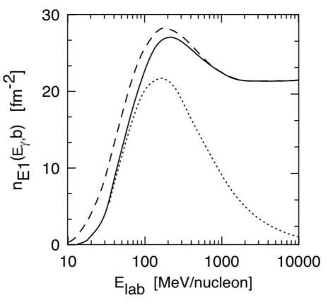
Figure 27: Electric dipole number of equivalent photons per unit area $d^{2}b\equiv 2\pi b\,db$, with energy of 10 MeV, incident on ²⁰⁸Pb in a collision with ¹⁶O at impact parameter $b=15$ fm, and as a function of the bombarding energy in MeV per nucleon. The dotted line and the dashed line correspond to calculations performed with the non-relativistic and with the relativistic approaches, respectively. The solid line represents a more correct calculation, as described in the text.

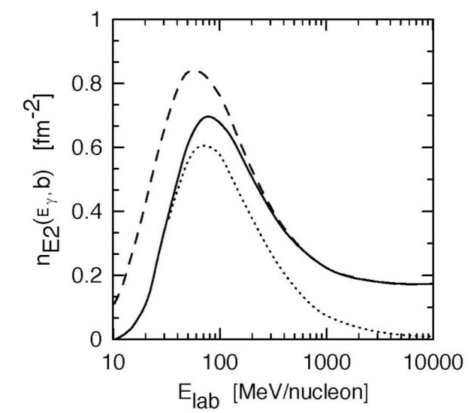
Figure 28: Same as Fig. 27, but for the $E2$ multipolarity.

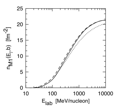
Figure 29: Same as Fig. 27, but for the $M1$ multipolarity.

As an example, we consider the excitations induced in ²⁰⁸Pb in ¹⁶O + ²⁰⁸Pb collisions. Since the expression (104), with Eqs. (107-108), is quite general, valid for all energies, the equivalent photon numbers contain all information about the differences among the low and the high energy scattering. In Figs. 27, 28 and 29 we show $dn_{\pi\lambda,\varepsilon}$, for the $E1$ (Fig. 27), $E2$ (Fig. 28), and $M1$ (Fig. 29) multipolarities, and for the collision ¹⁶O + ²⁰⁸Pb with an impact parameter $b=15\;$fm. They are the equivalent photon numbers with frequency $\omega=10\;$MeV$/\hbar$ incident on ²⁰⁸Pb. The dotted lines are obtained by using the non-relativistic Eq. (100), while the dashed lines correspond to the relativistic expressions (134,135,136). One observes that the relativistic expressions overestimate the equivalent photon numbers at low energies, while the non-relativistic expressions underestimate them at high energies. The correct values are given by the solid lines, calculated according to Eqs. (LABEL:3.27) and (225). They reproduce the low and the high energy limits, giving an improved interpolation between these limits at intermediate energies. These discrepancies are more apparent for the $E1$ and the $E2$ multipolarities. In the energy interval around 100A MeV neither the low energy theory nor the high energy one can reproduce well the correct values. This energy interval is indeed very sensitive to the effects of retardation and of Coulomb recoil.

At these bombarding energies, the differences between the magnitude of the non-relativistic and the correct relativistic virtual photon numbers are kept at a constant value, of about 20%, for excitation energies $E_{x}=\hbar\omega<10$ MeV. However, they increase sharply when one reaches the excitation energy of $E_{x}=\hbar\omega>10\;$MeV. The reason is that, for such excitation energies, the adiabaticity factor becomes greater than unity ($\xi>1$). This means that excitation energies of order of $10\;$MeV (like in the case of giant resonance excitation) are in the transition region from a constant behavior of the equivalent photon numbers to that of an exponential ($\sim e^{-\pi\xi}$) decay. This is more transparent in Fig. 13 where we plot the equivalent photon numbers for $E_{lab}=$100 MeV/nucleon, $b=15\;$fm, and as a function of $\hbar\omega$. One also observes from this figure that the $E2$ multipolarity component of the electromagnetic field dominates at low frequencies. Nonetheless, over the range of $\hbar\omega$ up to some tens of MeV, the $E2$ matrix elements of excitation are much smaller than the $E1$ elements for most nuclei, and the $E2$ effects become unimportant. However, such effects are relevant for the excitation of the isoscalar $E2$ giant resonance (GQR_is) which have large matrix elements.

Only for the $E1$ multipolarity the orbital integral in Eq. (LABEL:3.27) can be done analytically,

$${\frac{dn_{E1}}{d\Omega}} = {\frac{Z_{1}^{2}\alpha}{4\pi^{2}}}\;\bigl{(}{\frac{c}{v}}\bigr{)}^{2}\;{\epsilon^{4}\;\zeta^{2}}\;\;e^{-\pi\zeta}\;\biggl{\{}{\frac{1}{\gamma^{2}}}\;{\frac{\epsilon^{2}-1}{\epsilon^{2}}}\;\bigl{[}K_{i\zeta}({\epsilon\zeta})\bigr{]}^{2}$$ (226)

$$+ \bigl{[}K_{i\zeta}^{\prime}({\epsilon\zeta})\bigr{]}^{2}\biggr{\}}\,,$$

where $\epsilon=1/\sin(\vartheta/2)$, $\alpha=1/137$, $\zeta=\omega a_{0}/\gamma v$. $K_{i\zeta}$ is the modified Bessel function with imaginary index, $K_{i\zeta}^{\prime}$ is the derivative with respect to its argument. If one compares this equation with Eq. (113) one notes that besides the appearance of $\gamma$ factors in $a=a_{0}/\gamma$, the first term inside square brackets is also reduced by a $1/\gamma^{2}$, as compared to the non-relativistic expression. For relativistic energies, $\zeta\rightarrow 0$, $\epsilon\rightarrow\infty$, with $\zeta\epsilon\rightarrow{\rm const.}$. It is then easy to see that the above expression reduces to Eq. (134), in terms of the impact parameter dependence.

The integration over impact parameter can also be doen analytically for the $E1$ case. One obtains [BB88]

$$N_{E1} = {2\over\pi}\ Z_{1}^{2}\alpha\;e^{-\pi\zeta}\;\left({c\over v}\right)^{2}\;\Bigg{\{}-\xi K_{i\zeta}K_{i\zeta}^{\prime}-{1\over 2}\left({c\over v}\right)^{2}\xi^{2}$$

$$\times\Bigg{[}\left({\zeta\over\xi}\right)^{2}K_{i\zeta}^{2}+K_{i\zeta}^{\prime 2}-K_{i\zeta}^{2}$$

$$- \frac{i}{\epsilon_{0}}\left(K_{i\zeta}\left({{\partial K_{\mu}^{\prime}}\over{\partial\mu}}\right)_{\mu=i\zeta}-K_{i\zeta}^{\prime}\left({{\partial K_{\mu}}\over{\partial\mu}}\right)_{\mu=i\zeta}\right)\Bigg{]}\Bigg{\}}\ ,$$

where $\zeta=\omega a_{0}/\gamma v$,

$$\epsilon_{0}=\left\{\begin{array}[]{ll}1,&\mbox{for $2a>b_{mim}$ ,}\\ R/a-1,&\mbox{for $2a<b_{mim}$ ,}\end{array}\right.$$ (228)

and $\xi=\epsilon_{0}\zeta=\omega b_{mim}/\gamma v$.

It is easy to see that this equation reduces to Eq. (LABEL:(A.6a)) in the relativistic limit, when $\zeta\longrightarrow 0$, $\epsilon_{0}\longrightarrow\infty$. In practice, it is much easier to numerically calculate the orbital integrals in Eqs. (LABEL:3.27-225) directly. A numerical code (COULINT) is available for the purposes [Ber04].

IX E&M response of weakly-bound systems

Coulomb excitation has been one of the main tools to study the structure of unstable isotopes in radioactive beam facilities. This is a relatively new field and many new aspects of Coulomb excitation have been developed in the last two decades. We will discuss few of these aspects and, in particular, the role of transitions in/to the continuum of loosely-bound systems.

IX.1 Dominance of one resonance

It often occurs that the Coulomb excitation mechanism is dominated by transitions between the ground state and a continuum resonant state. This part of the excitation mechanism can be described exactly in a coupled-channels approach, while the other excitations can be described perturbatively [Ca96]. Fig. 30 represents the procedure. One resonance is coupled to the ground state while the remaining resonances are fed by these two states according to first order perturbation theory. The coupling matrix elements involves the ground state and a set of doorway states $|D_{\lambda\mu}^{(n)}>$ , where $n$  specifies the kind of resonance and $\lambda\mu$  are angular momentum quantum numbers. The amplitudes of these resonances in real continuum states are

$$\alpha^{(n)}(\epsilon)=<\phi(\epsilon)|\mathcal{D}_{\lambda\mu}^{(n)}>,$$ (229)

where $\phi(\epsilon)$  denotes the wavefunction of one of the numerous states which are responsible for the broad structure of the resonance. In this equation $\epsilon=E_{x}-E_{n}$ , where $E_{x}$  is the excitation energy and $E_{n}$  is the centroid of the resonance considered.

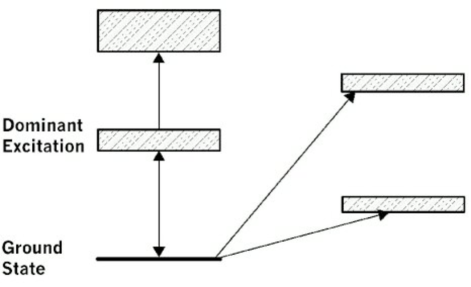
Figure 30: Schematic representation of Coulomb excitation of a dominant resonant state and of other states weakly-coupled to the ground state.

Let us assume for simplicity that the dominant resonant state has spin and parity $J^{P}=1^{-}$ . However, the following results can be easily generalized to all spin-parity types. The following coupled-channels equations are obtained [Ca96]:

$$i\hbar\frac{d{a}_{0}}{dt}(t) = \sum_{\mu}\int d\epsilon\left<\phi(\epsilon)|\mathcal{D}_{1\mu}^{(1)}\right>\left<\mathcal{D}_{1\mu}^{(1)}|V_{E1,\mu}(t)|0\right>$$ (230)

$$\times \exp\left\{-{\frac{i}{\hbar}}(E_{1}+\epsilon)t\right\}a_{\epsilon,1\mu}^{(1)}(t)$$

$$= \sum_{\mu}\int d\epsilon\ \alpha^{(1)}(\epsilon)\ V_{\mu}^{(01)}(t)\$$

$$\times \exp\left\{-{\frac{i}{\hbar}}(E+\epsilon)t\right\}\ a_{\epsilon,1\mu}^{(1)}(t),$$

and

$$i\hbar\ \frac{d{a}_{\epsilon,1\mu}^{(1)}}{dt}(t) = \left[(\alpha^{(1)}(\epsilon)\ V_{\mu}^{(01)}(t)\right]^{\ast}$$ (231)

$$\times \exp\left\{{i\over\hbar}(E_{1}+\epsilon)t\right\}\ a_{0}(t).$$

Above, $(n=1)$  stands for the dominant resonance, $a_{0}$denotes the occupation amplitude of the ground state and $a_{\epsilon,1\mu}^{(1)}$  the occupation amplitude of a state located at an energy $\epsilon$  away from the centroid of the resonance, and with magnetic quantum number $\mu$  ($\mu=-1,0,1$ ). We used the short hand notation $V_{\mu}^{(01)}(t)=\left<D_{1\mu}^{(1)}|V_{E1,\mu}(t)|0\right>$.

Integrating Eq. (231) and inserting the result in Eq. (230), we get the integro-differential equation for the ground state occupation amplitude

$$\frac{d^{2}{a}_{0}}{dt^{2}}(t)=-\frac{1}{\hbar^{2}}\sum_{\mu}\ V_{\mu}^{(01)}(t)\int d\epsilon|\alpha^{(1)}(\epsilon)|^{2}$$

$$\times \int_{-\infty}^{t}dt^{\prime}\left[V_{\mu}^{(01)}(t^{\prime})\right]^{\ast}\exp\left\{-{i\over\hbar}(E_{1}+\epsilon)(t-t^{\prime})\right\}a_{0}(t^{\prime}),$$

where we used that $a_{\epsilon,1\mu}^{(1)}(t=-\infty)=0$. To carry out the integration over $\epsilon$ , we should use an appropriate parametrization for the doorway amplitude $\alpha^{(1)}(\epsilon)$ . A convenient choice is the Breit-Wigner (BW) form which yields the square amplitude

$$|\alpha^{(1)}(\epsilon)|^{2}={\frac{1}{2\pi}}\ \left[{\frac{\Gamma_{1}}{\epsilon^{2}+\Gamma_{1}^{2}/4}}\right],$$ (233)

where $\Gamma_{1}$  is chosen to fit the experimental width. In this case, this integral will be the simple exponential

$$\int d\epsilon\ |\alpha^{(1)}(\epsilon)|^{2}\ \exp\left\{-i{\frac{(E_{1}+\epsilon)t}{\hbar}}\right\}$$ (234)

$$= \exp\left\{-i{\frac{(E_{1}-i\Gamma_{1}/2)t}{\hbar}}\right\}.$$

A better agreement with the experimental line shapes of the giant resonances is obtained by using a Lorentzian (L) parametrization for $|\alpha^{(1)}(\epsilon)|^{2}$ , i.e.,

$$|\alpha^{(1)}(\epsilon)|^{2}={\frac{2}{\pi}}\ \left[{\frac{\Gamma_{1}E_{x}^{2}}{(E_{x}^{2}-E_{1}^{2})^{2}+\Gamma_{1}^{2}E_{x}^{2}}}\right],$$ (235)

where $E_{x}=E_{1}+\epsilon$. The energy integral can still be performed exactly, but now it leads to the more complicated result

$$\int d\epsilon\ |\alpha^{(1)}(\epsilon)|^{2}\ \exp\left\{-i{\frac{(E_{1}+\epsilon)t}{\hbar}}\right\}$$ (236)

$$= \left(1-i{\frac{\Gamma_{1}}{2E_{1}}}\right)\ \exp\left\{-i{\frac{(E_{1}-i\Gamma_{1}/2)t}{\hbar}}\right\}\$$

$$+ \ \Delta C(t)\ ,$$

where $\Delta C(t)$  is a non-exponential correction to the decay. This correction can be shown numerically to be negligible. It will therefore be ignored. After integration over $\epsilon$ , Eq. (LABEL:da01) reduces to

$$\frac{d^{2}{a}_{0}}{dt^{2}}(t) = -\mathcal{S}_{1}\sum_{\mu}V_{\mu}^{(01)}(t)\int_{-\infty}^{t}dt^{\prime}\left[V_{\mu}^{(01)}(t^{\prime})\right]^{\ast}$$

$$\times \exp\left\{-i{\frac{(E_{1}-i\Gamma_{1}/2)(t-t^{\prime})}{\hbar}}\right\}a_{0}(t^{\prime})$$

where the factor $S_{1}$  is $S_{1}=1$  for BW-shape and $S_{1}=1-i\Gamma_{1}/2E_{1}$  for L-shape.

We can take advantage of the exponential time-dependence in the integral of the above equation, to reduce it to a set of second order differential equations. Introducing the auxiliary amplitudes $A_{\mu}(t)$, given by the relation

$$a_{0}(t)=1\ +\ \sum_{\mu}A_{\mu}(t),$$ (238)

with initial conditions $A_{\mu}(t=-\infty)=0$ , and taking the derivative of Eq. (238), one obtains

$${\ddot{A}}_{\mu}(t)-\left[{\frac{{\dot{V}}_{\mu}^{(01)}(t)}{V_{\mu}^{(01)}(t)}}\ -\ {\frac{i}{\hbar}}\left(E_{1}-i{\frac{\Gamma_{1}}{2}}\right)\right]{\dot{A}}_{\mu}(t)\$$ (239)

$$+ \ \mathcal{S}_{1}\ {\frac{|V_{\mu}^{(01)}(t)|^{2}}{\hbar^{2}}}\left[1+\sum_{\mu^{\prime}}A_{\mu^{\prime}}(t)\right]=0.$$

Solving the above equation, we get $a_{0}(t)$. Using this amplitude and integrating Eq. (231), one can evaluate $a_{\epsilon,1\mu}^{(1)}(t)$ . The probability density for the population of a dominant continuum state with energy $E_{x}$  in a collision with impact parameter $b$, $P_{1}(b,E_{x})$ , is obtained trough the summation over the asymptotic ($t\rightarrow\infty$ ) contribution from each magnetic substate. This yields

$$P_{1}(b,\ E_{x}) = |\alpha^{(1)}(E_{x}-E_{1})|^{2}\ \sum_{\mu}\Bigg{|}\int_{-\infty}^{\infty}dt^{\prime}$$ (240)

$$\times \exp\left\{iE_{x}t^{\prime}\right\}\ \left[V_{\mu}^{(01)}(t^{\prime})\right]^{\ast}\ a_{0}(t^{\prime})\Bigg{|}^{2},$$

where $|\alpha^{(1)}(E_{x}-E_{1})|^{2}$  is given by Eq. (233) or by Eq. (235), depending on the choice of the resonance shape.

To first order, the contribution to the excitation of another resonance (the one on the top of Fig. (30)) from the dominant one is given by

$$P_{2}(b,E_{x}) = |\alpha^{(2)}(E_{x}-E_{2})|^{2}\,\mathcal{S}_{1}$$

$$\times \sum_{\nu}\Bigg{|}\int_{-\infty}^{\infty}dt^{\prime}\exp\big{\{}iE_{x}t^{\prime}\big{\}}\ \sum_{\mu}\ \Big{[}V_{\nu\mu}^{(12)}(t^{\prime})\Big{]}^{\ast}$$

$$\times\int_{-\infty}^{t^{\prime}}dt^{\prime\prime}V_{\mu}^{(01)}(t^{\prime\prime})$$

$$\times \exp\Bigg{\{}-i{\frac{(E_{1}-i\Gamma_{1}/2)(t-t^{\prime})}{\hbar}}\Bigg{\}}\ a_{0}(t^{\prime\prime})\Bigg{|}^{2}.$$

We should point out that Eq. (LABEL:P2) is not equivalent to second-order perturbation theory. This would be true only in the limit $a_{0}(t)\longrightarrow 1$ . In this approach, $a_{0}(t)\neq 1$, since it is modified by the time-dependent coupling to the dominant state. This coupling is treated exactly by means of the coupled-channels equations. This approach is justified due to the (assumed) small excitation amplitude for the transition $1\longrightarrow 2$ , since $a_{1}(t)\ll a_{0}(t)$.

Equations similar to (240) can also be used to calculate the excitation probabilities directly from the ground-state, with the proper choice of energies, widths, and transition potentials. The above formalism has been used to study the excitation of giant resonances multiphonon resonances [Ca96]. It can be easily applied to description of pigmy resonances in nuclei far from the stability.

IX.2 Cluster-like light nuclei

In first-order perturbation theory, the photo-nuclear cross sections are related to the reduced matrix elements, for the excitation energy $E_{x}$ through the relation

$$\frac{d\sigma_{C}}{dE_{\gamma}}\left(E_{\gamma}\right)=\frac{(2\pi)^{3}(L+1)}{L\left[(2L+1)!!\right]^{2}}\left(\frac{E_{\gamma}}{\hbar c}\right)^{2L-1}\frac{dB}{dE_{x}}\left(\pi L,E_{\gamma}\right)$$ (242)

where $dB/dE_{x}$, are the reduced matrix elements, or Coulomb response functions.

The response function for electric transitions, $dB\left(EL\right)/dE_{\gamma},$ in Eq. (242) is given by

$$\frac{dB\left(EL\right)}{dE_{\gamma}}=\frac{\left|\left\langle J_{f}\left\|Y_{L}\left(\widehat{\mathbf{r}}\right)\right\|J_{i}\right\rangle\right|^{2}}{2J_{i}+1}$$ (243)

$$\times \left[\int_{0}^{\infty}dr\ r^{2+L}\ \ \delta\rho_{if}^{\left(EL\right)}\left(r\right)\right]^{2}w\left(E_{\gamma}\right),$$

where $w\left(E_{\gamma}\right)$ is the density of final states (for nuclear excitations into the continuum) with energy $E_{\gamma}=E_{f}-E_{i}$.

The transition density $\delta\rho_{if}^{\left(EL\right)}\left(r\right)$ will depend upon the nuclear model adopted. We will discuss here very simple models to calculate this response. To get a better reproduction of experimental data, more microscopic calculations such as the Random Phase Approximation (RPA) are often necessary.

IX.2.1 Cluster response function

Due to the small binding energy of nuclear halo systems composed of two clusters ($a=b+c$), the most important part of the wavefunction is beyond the range of the nuclear potential. The external part of the wavefunction is well described by an Yukawa of the form

$$\psi_{bc}(\mathbf{r})=N_{0}\sqrt{\frac{\eta}{2\pi}}\frac{e^{-\eta r}}{r}$$ (244)

where $\eta=\sqrt{2\mu_{bc}S/\hbar},$ $\mu_{bc}$ is the reduced mass of ($b+c$), $S$ is the separation energy, and $N_{0}=e^{\eta r_{0}}/\sqrt{1+\eta r_{0}}$ is a normalization factor which corrects the wavefunction to account for the finite range, $r_{0}$, of the ($b+c$) potential. There is no resonance structure in the $b+c$ continuum. This is clearly a good assumption for the deuteron and also for other neutron halo systems.

If we further assume that the final state is a plane-wave state (i.e., we neglect final state interactions) $\psi_{f}\equiv\left\langle\mathbf{q}|\mathbf{r}\right\rangle=e^{i\mathbf{q.r}}.$ The response functions for electric multipole transitions

$$\frac{dB}{dE_{x}}(E\lambda,E_{x})=SF\sum_{\mu}\Big{|}\left\langle\mathbf{q}\left|{\cal M}(ELM)\right|\psi_{bc}(\mathbf{r})\right\rangle\Big{|}^{2}\frac{d^{3}q}{(2\pi)^{3}}$$ (245)

where $SF$ is a spectroscopic factor (i.e., probability to find the system in the state ($b+c$)). ${\cal M}(ELM)$ is the electric multipole operator corrected to exclude c.m. motion, i.e.,

$${\cal M}(EL\mu) = e\sum\limits_{i=p}\left[\left(1-\frac{1}{A}\right)^{L}+(-1)^{L}\frac{\left(Z-1\right)}{A^{L}}\right]r_{i}^{L}Y_{L\mu}$$ (246)

$$+ \;e\sum_{i=n}\;Z\left(-\frac{1}{A^{L}}\right)r_{i}^{L}Y_{LM}$$

where the sum runs over all protons (p) and neutrons (n) in the nucleus.

For a cluster-system the sum runs over the (effective) charges of the clusters. For example,

$${\cal M}(E1M) = e\left(\frac{Z_{b}A_{c}-Z_{c}A_{b}}{A_{a}}\right)r_{bc}Y_{1M}(\widehat{\mathbf{r}}_{bc})$$

$${\cal M}(E2M) = e\left(\frac{Z_{b}A_{c}^{2}+Z_{c}A_{b}^{2}}{A_{a}^{2}}\right)r_{bc}Y_{2M}(\widehat{\mathbf{r}}_{bc})$$ (247)

where $\widehat{\mathbf{r}}_{bc}\;$is the relative position of b-c.

Using $d^{3}q=q^{2}dqd\Omega_{q}=\sqrt{2E_{x}}(\mu_{bc}/\hbar^{2})^{3/2}dEd\Omega_{q}$ in Eq. (245) and integrating over $\Omega,$ one finds [BS92]

$$\frac{dB(EL;E_{\gamma})}{dE_{\gamma}} = \frac{2^{L-1}}{\pi^{2}}(L!)^{2}(2L+1)(SF)N_{0}^{2}\left[O(L)\right]^{2}$$ (248)

$$\times \left(\frac{\hbar^{2}}{\mu_{bc}}\right)^{L}\frac{\sqrt{S}(E_{\gamma}-S)^{L+1/2}}{E_{\gamma}^{2L+2}}$$

where

$$O(L)=\frac{Z_{b}A_{c}^{L}-(-1)^{L}Z_{c}A_{b}^{L}}{A_{a}^{L}}\;e.$$ (249)

The maximum of this function occurs at

$$E_{0}^{EL}=\frac{L+1/2}{L+3/2}\;S.$$ (250)

In Figure 31 we show the photonuclear cross sections obtained by using Eq. (248) in the definition (242). The $E2$ and $E3$ photonuclear cross sections are smaller than the $E1$ by factors of order of 10⁵ and $10^{9}$, respectively. The spectroscopic factor and the normalization constant ($S$, and $N_{o}$, in Eq. (248) were set to unity, for simplicity. The have a longer tail than the $E1$ photonuclear cross section due to the factor $E_{x}^{2L-1}$ in Eq. (242). Thus, we conclude that a cluster-like correlation is not as effective in producing an enhancement of the low energy part of the photonuclear cross sections for higher multipolarities, as in the dipole case.

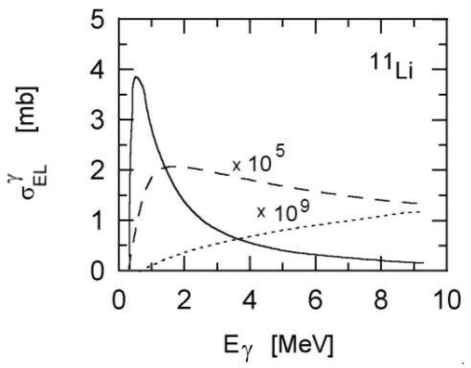
Figure 31: Photo absorption cross section of ¹¹Li in the cluster model. The solid (dashed) [dotted] curve corresponds to dipole (quadrupole) [octupole] multipolarity. The quadrupole (octupole) values were multiplied by a factor of $10^{5}$ (10⁹) [BS92].

IX.2.2 One-neutron halo

We will now discuss the effect of final state interactions. We start by considering a one-neutron halo nucleus. The initial wavefunction can be written as $\Psi_{JM}=r^{-1}u_{ljJ}(r)\mathcal{Y}_{lJM}$, where $R_{ljJ}(r)$ is the radial wavefunction and $\mathcal{Y}_{lJM}$ is a spin-angle function [BD04].

As before, we use a simple Yukawa form for an s-wave initial wavefunction, $u_{0}(r)=N_{0}\exp(-\eta r)$, and a p-wave final wavefunction, $\ u_{1}(r)=j_{1}(kr)\cos\delta_{1}-\ n_{1}(kr)\sin\delta_{1}$. In these equations $\eta$ is related to the neutron separation energy $S_{n}=\hbar^{2}\eta^{2}/2\mu$, $\mu$ is the reduced mass of the neutron + core system, and $\hbar k=\sqrt{2\mu E_{r}}$, with $E_{r}$ being the final energy of relative motion between the neutron and the core nucleus. $N_{0}$ is the normalization constant of the initial wavefunction.

The transition density is given by $r^{2}\delta\rho_{if}\left(r\right)=e_{eff}A_{i}u_{i}(r)u_{f}(r)$, where $i$ and $f$ indices include angular momentum dependence and $e_{eff}=-eZ_{c}/A$ is the effective charge of a neutron+core nucleus with charge $Z_{c}$. The $E1$ transition integral $\mathcal{I}_{l_{i}l_{f}}=\int_{0}^{\infty}dr\ r^{3}\ \ \delta\rho_{if}\left(r\right)$ for the wavefunctions described above yields

$$\mathcal{I}_{s\rightarrow p} =e_{eff}\frac{2k^{2}}{\left(\eta^{2}+k^{2}\right)^{2}}\left[\cos\delta_{1}+\sin\delta_{1}\frac{\eta\left(\eta^{2}+3k^{2}\right)}{2k^{3}}\right]$$

$$\simeq\frac{e_{eff}\hbar^{2}}{2\mu}\frac{2E_{r}}{\left(S_{n}+E_{r}\right)^{2}}\Bigg{[}1+$$

$$\left(\frac{\mu}{2\hbar^{2}}\right)^{3/2}\frac{\sqrt{S_{n}}\left(S_{n}+3E_{r}\right)}{-1/a_{1}+\mu r_{1}E_{r}/\hbar^{2}}\Biggr{]},$$ (251)

where the effective range expansion of the phase shift, $k^{2l+1}\cot\delta\simeq-1/a_{l}+r_{l}k^{2}/2,$ was used in the second line of the above equation. For $l=1$, $a_{1}$ is the “scattering volume” (units of length³) and $r_{1}$ is the “effective momentum” (units of 1/length). Their interpretation is not as simple as the $l=0$ effective range parameters. Typical values are, e.g. $a_{1}=-13.82$ fm^-3 and $r_{1}=-0.419$ fm^-1 for n+⁴He $p_{1/2}$-wave scattering and $a_{1}=-62.95$ fm^-3 and $r_{1}=-0.882$ fm^-1 for n+⁴He $p_{3/2}$-wave scattering [Arn73].

The energy dependence of Eq. (251) has some unique features. As shown in the previous section, the matrix elements for electromagnetic response of weakly-bound nuclei present a small peak at low energies, due to the proximity of the bound state to the continuum. This peak is manifest in the response function as

$$\frac{dB(EL)}{dE}\propto\left|\mathcal{I}_{s\rightarrow p}\right|^{2}\propto\frac{E_{r}^{L+1/2}}{\left(S_{n}+E_{r}\right)^{2L+2}}.$$ (252)

It appears centered at the energy [BS92] $E_{0}^{(EL)}\simeq\frac{L+1/2}{L+3/2}S_{n}$ for a generic electric response of multipolarity $L$. For $E1$ excitations, the peak occurs at $E_{0}\simeq 3S_{n}/5$.

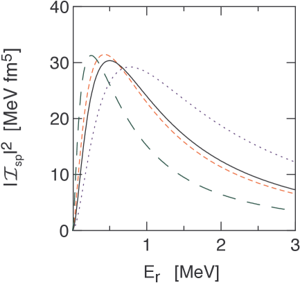
Figure 32: $\left|\mathcal{I}_{s\rightarrow p}\right|^{2}$  calculated using Eq. (251), assuming $e_{eff}=e$, $A=11$ and $S_{n}=0.5$ MeV, as a function of $E_{r}$, the relative energy of the fragments. The long dashed curve corresponds to  $a_{1}=-10$ fm^-3 and $r_{1}=-0.5$ fm^-1, the dashed curve corresponds to  $a_{1}=-50$ fm^-3 and $r_{1}=1$ fm${}^{-1},$ the solid curve corresponds to $a_{1}=$ $r_{1}=0$, and finally, the dotted curve corresponds to $a_{1}=-10$ fm^-3 and $r_{1}=0.5$ fm^-1.

The second term inside brackets in Eq. (251) is a modification due to final state interactions. This modification may become important, as shown in figure 32, where $\left|\mathcal{I}_{s\rightarrow p}\right|^{2}$ calculated with Eq. (251) is plotted as a function of $E_{r}$. Here, for simplicity, we have assumed the values $e_{eff}=e$, $A=11$ and $S_{n}=0.5$ MeV. This does not correspond to any known nucleus and is used to assess the effect of the scattering length and effective range in the transition matrix element. The long dashed curve corresponds to  $a_{1}=-10$ fm^-3 and $r_{1}=-0.5$ fm^-1, the dashed curve corresponds to  $a_{1}=-50$ fm^-3 and $r_{1}=1$ fm${}^{-1},$ the solid curve corresponds to $a_{1}=$ $r_{1}=0$, and finally, the dotted curve corresponds to $a_{1}=-10$ fm^-3 and $r_{1}=0.5$ fm${}^{-1}.$ Although the effective range expansion is only valid for small values of $E_{r}$, it is evident from the figure that the matrix element is very sensitive to the effective range expansion parameters.

The strong dependence of the response function on the effective range expansion parameters makes it an ideal tool to study the scattering properties of light nuclei which are of interest for nuclear astrophysics. It is important to notice that the one-halo has been studied in many experiments, e.g. for the case of ¹¹Be for which there are many data available. In the literature one can find a detailed analysis of how the nuclear shell-model can explain the experimental data, by fitting the spectroscopic factors for several single-particle configurations.

IX.2.3 Two-neutron halo

Weakly-bound nuclei, such ⁶He or ¹¹Li, require a three–body treatment in order to reproduce the electromagnetic response more accurately. In a popular three-body model, the bound–state wavefunction in the center of mass system is written as an expansion over hyperspherical harmonics (HH), see e.g. [Zhu93],

$$\Psi\left(\mathbf{x},\mathbf{y}\right)=\frac{1}{\rho^{5/2}}\sum_{KLSl_{x}l_{y}}\Phi_{KLS}^{l_{x}l_{y}}\left(\rho\right)\left[\mathcal{J}_{KL}^{l_{x}l_{y}}\left(\Omega_{5}\right)\otimes\chi_{S}\right]_{JM}.$$ (253)

Here $\mathbf{x}$ and $\mathbf{y}$ are Jacobi vectors where (see figure 33) $\mathbf{x}=\frac{1}{\sqrt{2}}\left(\mathbf{r}_{1}-\mathbf{r}_{2}\right)$ and $y=\sqrt{\frac{2\left(A-2\right)}{A}}\left(\frac{\mathbf{r}_{1}+\mathbf{r}_{2}}{2}-\mathbf{r}_{c}\right)$, where A is the nuclear mass, $\mathbf{r}_{1}$ and $\mathbf{r}_{2}$ are the position of the nucleons, and $\mathbf{r}_{c}$ is the position of the core. The hyperradius  $\rho$ determines the size of a three-body state: $\rho^{2}=x^{2}+y^{2}$. The five angles $\left\{\Omega_{5}\right\}$ include usual angles $(\theta_{x},\phi_{x})$, $(\theta_{y},\phi_{y})$ which parametrize the direction of the unit vectors $\widehat{\mathbf{x}}$ and $\widehat{\mathbf{y}}$ and the hyperangle $\theta$, related by $x=\rho\sin\theta$ and $y=\rho\cos\theta$, where $0\leq\theta\leq\pi/2$.

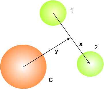
Figure 33: Jacobian coordinates (x and y) for a three-body system consisting of a core (c) and two nucleons (1 and 2).

The insertion of the three-body wavefunction, Eq. (253), into the Schrödinger equation yields a set of coupled differential equations for the hyperradial wavefunction $\Phi_{KLS}^{l_{x}l_{y}}\left(\rho\right)$. Assuming that the nuclear potentials between the three particles are known, this procedure yields the bound-state wavefunction for a three-body system with angular momentum $J$.

In order to calculate the electric response we need the scattering wavefunctions in the three-body model to calculate the integrals in Eq. (243). One would have to use final wavefunctions with given momenta, including their angular information. When the final state interaction is disregarded these wavefunctions are three-body plane waves [Pus96]. To carry out the calculations, the plane waves can be expanded in products of hyperspherical harmonics in coordinate and momentum spaces. However, since we are only interested in the energy dependence of the response function, we do not need directions of the momenta. Thus, instead of using plane waves, we will use a set of final states which just include the coordinate space and energy dependence.

For weakly-bound systems having no bound subsystems the hyperradial functions entering the expansion (253) behave asymptotically as [Mer74] $\Phi_{a}\left(\rho\right)\longrightarrow\text{constant}\times\ \exp\left(-\eta\rho\right)$ as $\rho\longrightarrow\infty$, where the two-nucleon separation energy is related to $\eta$ by $S_{2n}=\hbar^{2}\eta^{2}/\left(2m_{N}\right)$. This wavefunction has similarities with the two-body case, when $\rho$ is interpreted as the distance $r$ between the core and the two nucleons, treated as one single particle. But notice that the mass $m_{N}$ would have to be replaced by $2m_{N}$ if a simple two-body (the dineutron-model [BB88]) were used for ¹¹Li or ⁶He.

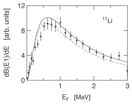
Figure 34: Comparison between the calculation of the response function (in arbitrary units) with eqs. (254) and (255), using $\delta_{nn}=0$ and $\delta_{nc}=0$, (dashed line), or including the effects of final state interactions (continuous line). The experimental data are from Ref. [Shi95].

Since only the core carries charge, in a three-body model the $E1$ transition operator is given by $M\sim yY_{1M}\left(\widehat{\mathbf{y}}\right)$ for the final state. The $E1$ transition matrix element is obtained by a sandwich of this operator between $\Phi_{a}\left(\rho\right)/\rho^{5/2}$ and scattering wavefunctions. In Ref. [Pus96] the scattering states were taken as plane waves. We will use distorted scattering states, leading to the expression

$$\mathcal{I}\left(E1\right)=\int dxdy\frac{\Phi_{a}\left(\rho\right)}{\rho^{5/2}}\ y^{2}xu_{p}\left(y\right)u_{q}\left(x\right),$$ (254)

where $u_{p}\left(y\right)=j_{1}\left(py\right)\cos\delta_{nc}-n_{1}\left(py\right)\sin\delta_{nc}$ is the core-neutron asymptotic continuum wavefunction, assumed to be a $p$-wave, and $u_{q}\left(x\right)=j_{0}\left(qx\right)\cos\delta_{nn}-n_{0}\left(qx\right)\sin\delta_{nn}$ is the neutron-neutron asymptotic continuum wavefunction, assumed to be an $s$-wave. The relative momenta are given by $\mathbf{q}=\frac{1}{\sqrt{2}}\left(\mathbf{q}_{1}-\mathbf{q}_{2}\right)$, and $\mathbf{p}=\sqrt{\frac{2\left(A-2\right)}{A}}\left(\frac{\mathbf{k}_{1}+\mathbf{k}_{2}}{2}-\mathbf{k}_{c}\right)$.

The $E1$ strength function is proportional to the square of the matrix element in Eq. (254) integrated over all momentum variables, except for the total continuum energy $E_{r}=\hbar^{2}\left(q^{2}+p^{2}\right)/2m_{N}$. This procedure gives

$$\frac{dB\left(E1\right)}{dE_{r}} = \text{constant }\cdot\int\left|\mathcal{I}\left(E1\right)\right|^{2}E_{r}^{2}\cos^{2}\Theta$$ (255)

$$\times \sin^{2}\Theta d\Theta d\Omega_{q}d\Omega_{p},$$

where $\Theta=\tan^{-1}\left(q/p\right)$.

The ¹S₀ phase shift in neutron-neutron scattering is remarkably well reproduced up to center of mass energy of order of 5 MeV by the first two terms in the effective-range expansion $k\cot\delta_{nn}\simeq-1/a_{nn}+r_{nn}k^{2}/2.$ Experimentally these parameters are determined to be $a_{nn}=-23.7$ fm and $r_{nn}=2.7$ fm. The extremely large (negative) value of the scattering length implies that there is a virtual bound state in this channel very near zero energy. The p-wave scattering in the n-⁹Li (¹⁰Li) system appears to have resonances at low energies [Thoe99]. We assume that this phase-shift can be described by the resonance relation$\sin\delta_{nc}=({\Gamma/2})/{\sqrt{\left(E_{r}-E_{R}\right)^{2}+\Gamma^{2}/4}}$, with $E_{R}=0.53$ MeV and $\Gamma=0.5$ MeV [Thoe99].

Most integrals in eqs. (254) and (255) can be done analytically, leaving two remaining integrals which can only be performed numerically. The result of the calculation is shown in figure (34). The dashed line was obtained using $\delta_{nn}=0$ and $\delta_{nc}=0$, that is, by neglecting final state interactions. The continuous curve includes the effects of final state interactions, with $\delta_{nn}$ and $\delta_{nc}$ parametrized as described above. The experimental data are from Ref. [Shi95]. The data and theoretical curves are given in arbitrary units. Although the experimental data is not perfectly described by either one of the results, it is clear that final state interactions are of extreme relevance.

As pointed out in Ref. [Pus96], the $E1$ three-body response function of ¹¹Li can still be described by an expression similar to Eq. (252), but with different powers. Explicitly, ${dB\left(E1\right)}/{dE_{r}}\propto{E_{r}^{3}}/{\left(S_{2n}^{eff}+E_{r}\right)^{11/2}}$. Instead of $S_{2n}$, one has to use an effective $S_{2n}^{eff}=aS_{2n}$, with $a\simeq 1.5$. With this approximation, the peak of the strength function in the three-body case is situated at about three times higher energy than for the two-body case, Eq. (252). In the three-body model, the maximum is thus predicted at $E_{0}^{(E1)}\simeq 1.8S_{2n}$, which fits the experimentally determined peak position for the ¹¹Li $E1$ strength function very well [Pus96]. It is thus apparent that the effect of three-body configurations is to widen and to shift the strength function $dB\left(E1\right)/dE$ to higher energies.

It is worthwhile mentioning that the data presented in figure 34, and of other experiments, is different in form and magnitude of the more recent experiment of Ref. [Nak06]. The reason for the discrepancy is attributed to an enhanced sensitivity in the experiment of Ref. [Nak06] to low relative energies below $E_{rel}=0.5$ MeV compared to previous experiments. Also, this recent experiment agrees very well with the nn-correlated model of Ref. [EB92]. This theoretical model is different than the model presented in this section in many aspects. In principle, the three-body models should be superior, as they include the interactions between the three-particles without any approximation. For example, Ref. [EB92] use a simplified interaction between the two-neutrons. On the other hand, they include the many-body effects, e.g. the Pauli blocking of the occupied states in the core. It is not well known the reason why the data of Ref. [Nak06] is better described with the model of Ref. [EB92] than traditional 3-body models.

IX.3 Pigmy resonances

We have seen that the energy position where the soft dipole response peaks depends upon the few body model adopted. Except for a two-body resonance in ¹⁰Li, there was no reference to a resonance in the continuum. The peak in the response function can be simply explained by the fact that it has to grow from zero at low energies and return to zero at large energies. In few-body, or cluster, models, the form of the bound-state wavefunctions and the phase space in the continuum determine the position of the peak in the response function. Few-body resonances will lead to more peaks.

Now we shall consider the case in which a collective resonance is present. As with giant dipole resonances (GDR) in stable nuclei, one believes that pygmy resonances at energies close to the threshold are present in halo, or neutron-rich, nuclei (in English, pigmy = pygmy). This was proposed in Ref. [SIS90] using the hydrodynamical model for collective vibrations. The possibility to explain the soft dipole modes (figure 34) in terms of direct breakup, has made it very difficult to clearly identify the signature of pygmy resonances in light exotic nuclei.

The hydrodynamical model needs adjustments to explain collective response in light, neutron-rich, nuclei. Because clusterization in light nuclei exists, not all neutrons and protons can be treated equally. The necessary modifications are straight-forward and discussed next.

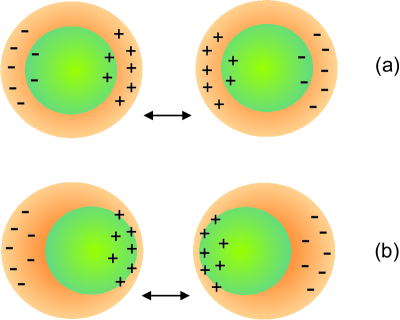
Figure 35: Hydrodynamical model for collective nuclear vibrations in halo nuclei. The (a) Steinwedel-Jensen (SJ) mode and the (b) Goldhaber-Teller (GT) mode are shown separately.

When a collective vibration of protons against neutrons is present in a nucleus with charge (neutron) number $Z$ ($N$), the neutron and proton fluids are displaced with respect to each other by $d_{1}=\alpha_{1}R$ and each of the fluids are displaced from the origin (center of mass of the system) by $d_{p}=Nd_{1}/A$ and $d_{n}=-Zd_{1}/A$. This leaves the center of mass fixed and one gets for the dipole moment $D_{1}=Zed_{p}=\alpha_{1}NZeR/A$. The GT (Goldhaber-Teller) model [Gt48] assumes that the restoring force is due to the increase of the nuclear surface which leads to an extra energy proportional to $A^{2/3}$. In this model, the inertia is proportional to $A$ and the excitation energy is consequently given by $E_{x}\propto\sqrt{A^{2/3}/A}=A^{-1/6}$.

For light, weakly-bound nuclei, it is more appropriate to assume that the neutrons inside the core ($A_{c},Z_{c}$) vibrate in phase with the protons. The neutrons and protons in the core are tightly bound. An overall displacement among them requires energies of the order of 10-20 MeV, well above that of the soft dipole modes. The dipole moment becomes $\mathbf{D}_{1}=e\mathbf{d}_{1}{\left(Z_{c}A-ZA_{c}\right)}/{A}=Z_{eff}^{(1)}e\mathbf{d}_{1}$, where $\mathbf{d}_{1}$ is a vector connecting the center of mass of the two fluids (core and excess neutrons). We see that the dipole moment is now smaller than before because the effective charge changes from $NZ/A$ in the case of the GDR to $Z_{eff}^{(1)}=$ $\left(Z_{c}A-ZA_{c}\right)/A$. This effective charge is zero if $Z_{c}A=ZA_{c}$ and no pigmy resonance is possible in this model, only the usual GDR.

Figure 35 shows a schematic representation of the hydrodynamical model for collective nuclear vibrations in a halo nucleus, as considered here. Part (a) of the figure shows the Steinwedel-Jensen (SJ) mode [SJ50] in which the total matter density of both the core and the halo nucleons do not change locally. Only the local ratio of the neutrons and protons changes. Part (b) of the figure shows a particular case of the Goldhaber-Teller (GT) mode, in which the core as a whole moves with respect to the halo nucleons.

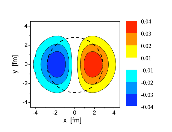
Figure 36: Contour plot of the nuclear transition density in the hydrodynamical model consisting of a mixture of GT and SJ vibrations. The darker areas represent the larger values of the transition density in a nucleus which has an average radius represented by the dashed circle. The legend on the right displays the values of the transition density within each contour limit.

For spherically symmetric densities, the transition density in the GT mode can be calculated from $\delta\rho_{p}=\rho_{p}\left(\left|\mathbf{r}-\mathbf{d}_{p}\right|\right)-\rho_{p}\left(\mathbf{r}\right)$, where $\rho_{p}$ is the charge density. Using $d_{1}\ll R$, it is straight-forward to show that $\delta\rho_{p}^{(1)}\left(\mathbf{r}\right)=\delta\rho_{p}^{(1)}\left(r\right)Y_{10}\left(\widehat{\mathbf{r}}\right)$ , where

$$\delta\rho_{p}^{(1)}\left(r\right)=\sqrt{\frac{4\pi}{3}}Z_{eff}\alpha_{1}R\frac{d\rho_{0}}{dr},$$ (256)

and $\rho_{0}$ is the ground state matter density.

In the Steinwedel-Jensen (SJ) mode, the local variation of the density of protons is found to be $\delta\rho_{p}^{(2)}\left(\mathbf{r}\right)=\delta\rho_{p}^{(2)}\left(r\right)Y_{10}\left(\widehat{\mathbf{r}}\right)$, where

$$\delta\rho_{p}^{(2)}\left(r\right)=\sqrt{\frac{4\pi}{3}}Z_{eff}^{(2)}\alpha_{2}Kj_{1}\left(kr\right)\rho_{0}\left(r\right),$$ (257)

where $K=9.93$. If the proton and neutron content of the core does not change [SIS90], the effective charge number in the SJ mode is given by $Z_{eff}^{(2)}=Z^{2}(N-N_{c})/A(Z+N_{c})$.

The transition density at a point $\mathbf{r}$ from the center-of-mass of the nucleus is a combination of the SJ and GT distributions and is given by $\delta\rho_{p}\left(\mathbf{r}\right)=\delta\rho_{p}\left(r\right)Y_{10}\left(\widehat{\mathbf{r}}\right)$, where

$$\delta\rho_{p}\left(r\right)=\sqrt{\frac{4\pi}{3}}R\left\{Z_{eff}^{(1)}\alpha_{1}\frac{d}{dr}+Z_{eff}^{(2)}\alpha_{2}\frac{K}{R}j_{1}\left(kr\right)\right\}\rho_{0}(r).$$ (258)

Changes can be accommodated in these expressions to account for the different radii of the proton and neutron densities.

Figure 36 shows the contour plot, in arbitrary units, of the nuclear transition density in the hydrodynamical model, consisting of a mixture of GT and SJ vibrations. The darker areas represent the larger values of the transition density in a nucleus which has an average radius represented by the dashed circle. In this particular case, a Hartree-Fock density calculation for ¹¹Li, and a radius $R=3.1$ fm, was used. The parameters $\alpha_{1}$ and $\alpha_{2}$ were chosen so that $Z_{eff}^{(1)}\alpha_{1}=Z_{eff}^{(2)}\alpha_{2}$, i.e. a symmetric mixture of the SJ and GT modes.

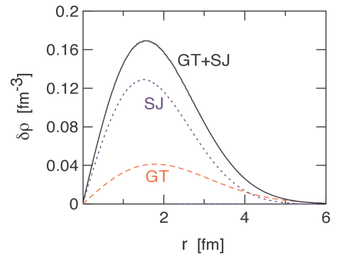
Figure 37: Hydrodynamical transition densities for ¹¹Li and three different assumptions for the SJ+GT admixtures, according to Eq. (258). The dashed curve is for a GT oscillation mode, with the core vibrating against the halo neutrons, with effective charge number $Z_{eff}^{(1)}=6/11$, radius $R=3.1$ fm, and $\alpha_{1}=1$. The dotted curve is for an SJ oscillation mode, with effective charge number $Z_{eff}^{(2)}=2/11$, and $\alpha_{2}=1$. The solid curve is their sum.

Figure 37 shows the transition densities for ¹¹Li for three different assumptions of the SJ+GT admixtures, according to Eq. (258). The dashed curve is for a GT oscillation mode, with the core vibrating against the halo neutrons, with effective charge number $Z_{eff}^{(1)}=6/11$, radius $R=3.1$ fm, and $\alpha_{1}=1$. The dotted curve is for an SJ oscillation mode, with effective charge number $Z_{eff}^{(2)}=2/11$, and $\alpha_{2}=1$. The solid curve is their sum. Notice that the transition densities are peaked at the surface, but at a radius smaller than the adopted “rms” radius $R=3.1$ fm.

The liquid drop model predicts an equal admixture of SJ+GT oscillation modes for large nuclei [Mye77]. The contribution of the SJ oscillation mode decreases with decreasing mass number, i.e. $\alpha_{2}\longrightarrow 0$ as $A\longrightarrow 0$. This is even more probable in the case of halo nuclei, where a special type of GT mode (oscillations of the core against the halo nucleons) is likely to be dominant. For this special collective motion an approach different than that used in Ref. [SIS90] has to be considered. The resonance energy formula derived by Goldhaber and Teller [GT48] changes to

$$E_{PR}=\left(\frac{3\varphi\hbar^{2}}{2aRm_{N}A_{r}}\right)^{1/2},$$ (259)

where $A_{r}=A_{c}\left(A-A_{c}\right)/A$ and $a$ is the length within which the interaction between a neutron and a nucleus changes from a zero-value outside the nucleus to a high value inside, i.e. $a$ is the size of the nuclear surface. $\varphi$ is the energy needed to extract one neutron from the proton environment.

Goldhaber and Teller [GT48] argued that in a heavy stable nucleus $\varphi$ is not the binding energy of the nucleus, but the part of the potential energy due to the neutron-proton interaction. It is proportional to the asymmetry energy. In the case of weakly-bound nuclei this picture changes and it is more reasonable to associate $\varphi$ to the separation energy of the valence neutrons, $S$. I will use $\varphi=\beta S$, with a parameter $\beta$ which is expected to be of order of one. Since for halo nuclei the product $aR$  is proportional to $S^{-1},$ we obtain the proportionality $E_{PR}\propto S$. Using Eq. (259) for ¹¹Li , with  $a=1$ fm, $R=3$ fm and $\varphi=S_{2n}=0.3$ MeV, we get $E_{PR}=1.3$ MeV. Considering that the pygmy resonance will most probably decay by particle emission, one gets $E_{r}\simeq 1$ MeV for the kinetic energy of the fragments, which is within the right ballpark (see figure 34).

Both the direct dissociation model and the hydrodynamical model yield a bump in the response function proportional to $S$, the valence nucleon(s) separation energy. In the direct dissociation model the width of the response function obviously depends on the separation energy. But it also depends on the nature of the model, i.e. if it is a two-body model, like the model often adopted for ¹¹Be or ⁸B, or a three-body model, appropriate for ¹¹Li and ⁶He. In the two-body model the phase-space depends on energy as $\rho\left(E\right)\propto d^{3}p/dE\propto\sqrt{E}$, while in the three-body model $\rho\left(E\right)\sim E^{2}$. This explains why the peak of figure 34 is pushed toward higher energy values, as compared to the prediction of Eq. (252). It also explains the larger width of $dB/dE$ obtained in three-body models. In the case of the pigmy resonance model, this question is completely open.

The hydrodynamical model predicts [Mye77] for the width of the collective mode $\Gamma=\hbar\overline{\mathrm{v}}/R$, where $\overline{\mathrm{v}}$  is the average velocity of the nucleons inside the nucleus. This relation can be derived by assuming that the collective vibration is damped by the incoherent collisions of the nucleons with the walls of the nuclear potential well during the vibration cycles (piston model). Using $\overline{\mathrm{v}}=3\mathrm{v}_{F}/4$, where $\mathrm{v}_{F}=\sqrt{2E_{F}/m_{N}}$ is the Fermi velocity, with $E_{F}=35$ MeV and $R=6$ fm, one gets $\Gamma\simeq 6$ MeV. This is the typical energy width a giant dipole resonance state in a heavy nucleus. In the case of neutron-rich light nuclei $\overline{\mathrm{v}}$ is not well defined. There are two average velocities: one for the nucleons in the core, $\overline{\mathrm{v}}_{c}$, and another for the nucleons in the skin, or halo, of the nucleus, $\overline{\mathrm{v}}_{h}$. One is thus tempted to use a substitution in the form $\overline{\mathrm{v}}=\sqrt{\overline{\mathrm{v}}_{c}\overline{\mathrm{v}}_{h}}.$ Following Ref. [BM93], the width of momentum distributions of core fragments in knockout reactions, $\sigma_{c}$, is related to the Fermi velocity of halo nucleons by $\mathrm{v}_{F}=\sqrt{5\sigma_{c}^{2}}/m_{N}$. Using this expression with $\sigma_{c}\simeq 20$ MeV/c, we get $\Gamma=5$  MeV (with $R=3$ fm). This value is also not in discordance with experiments (see figure 34).

Better microscopic models, e.g. those based on random phase approximation (RPA) calculations are necessary to study pigmy resonances. The halo nucleons have to be treated in an special way to get the response at the right energy position, and with approximately the right width.

IX.4 Comparison between cluster breakup and pigmy resonance excitation

One might argue that the total breakup cross section would be a good signature for discerning direct dissociation versus the dissociation through the excitation of a pigmy collective vibration. The trouble is that the energy weighted sum rule for both cases are approximately of the same magnitude. This can be shown by using the electric dipole strength function in the cluster breakup model, namely

$$\frac{dB(E1)}{dE}=\mathcal{C}\frac{3\hbar e^{2}Z_{eff}^{2}}{\pi^{2}\mu}\frac{\sqrt{S_{n}}\left(E-S_{n}\right)^{3/2}}{E^{4}},$$ (260)

where $E=E_{r}+S_{n}$ is the total excitation energy. $\mathcal{C}$ is a constant of the order of one, accounting for the corrections to the wavefunction.

The sum rule for dipole excitations, $S_{1}\left(E1\right)=\int_{S_{n}}^{\infty}dE\ E\ \frac{dB\left(E1\right)}{dE}$, is

$$S_{1}\left(E1\right)=\mathcal{C}\left(\frac{9}{8\pi}\right)\frac{\hbar^{2}e^{2}}{\mu}Z_{eff}^{2},$$ (261)

with $Z_{eff}^{2}=\left(Z_{c}A-ZA_{c}\right)^{2}/[AA_{c}\left(A-A_{c}\right)]$. This is the same (with $\mathcal{C}=1$) as Eq. 1 of Ref. [AGB82], which is often quoted as the standard value to which models for the nuclear response in the region of pigmy resonance should be compared to. The response function in Eq. (260), with $\mathcal{C}=1$, therefore exhausts 100% of the so-called cluster sum rule [AGB82]. The total cross section for electron breakup of weakly-bound systems is roughly proportional to $S_{1}$. This assertion can be easily verified by using eqs. (353) and (260), assuming that the logarithmic dependence of the virtual photon numbers on the energy $E\equiv E_{\gamma}$ can be factored out of the integral in Eq. (353).

The dipole strength of the pigmy dipole resonance is given by the same equation (261). The constant $\mathcal{C}$ is still of the order of unity, but not necessarily the same as in Eq. (260) and the effective charges are also different. For the Goldhaber-Teller pigmy dipole model the effective charge is given by $Z_{eff}^{(1)}=$ $\left(Z_{c}A-ZA_{c}\right)/A$, whereas for the Steinwedel-Jensen it is $Z_{eff}^{(2)}=(Z^{2}/A)(N-N_{c})/(Z+N_{c})$. Assuming that the Goldhaber-Teller mode prevails, one gets the simple prediction for the ratio between the cross sections for direct breakup versus excitation of a pigmy collective mode:

$$\frac{\sigma^{direct}}{\sigma^{pigmy}}=\mathcal{C}\frac{A}{A_{c}\left(A-A_{c}\right)}.$$ (262)

For ¹¹Li this ratio is 11$\mathcal{C}$/18 while for ¹¹Be it is 11$\mathcal{C}$/10. One thus concludes that it is very difficult to identify if the nuclear response at low energies is due to collective excitations of pigmy resonances, or a trivial phase-space effect due to the cluster dissociation, which is a basic manifestation of the low binding energy. Other observables are necessary to make firm conclusions, such as correlations of emitted fragments.

IX.5 Higher-order effects

Breakup processes in nucleus-nucleus collisions are complicated, in whatever way they are treated. They constitute at least a three-body problem, which is further complicated due to the long range Coulomb force. Exact treatments (such as the Fadeev-approach) are therefore prohibitively cumbersome. On the other hand, many approximate schemes have been developed and these approaches have been used with considerable success.

Higher-order effects in Coulomb breakup were first observed in Ref. [Ie93]. In Fig. 38 we see that the velocity of ⁹Li fragments are faster, in average, than those of the two detached neutrons in a Coulomb break-up of 28 MeV/nucleon ¹¹Li incident on lead targets.

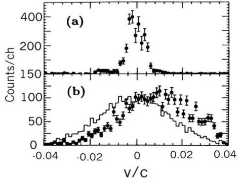
Figure 38: Spectrum of the longitudinal component of the center-of-mass velocity of ⁹Li and two neutrons in the frame of the incident ¹¹Li. (b) Spectrum of the longitudinal component of the relative velocity V₉ - V${}_{2n}.$ The histogram shows the result of a Monte Carlo simulation assuming no Coulomb acceleration effects.

This effect can be understood qualitatively as follows. The ¹¹Li is deccelerated up to a point where it dissociates. This occurs around the distance of closest approach. Afterwards the ⁹Li fragments is accelerated, whereas the neutrons are not. Since ⁹Li is lighter than ¹¹Li its final velocity is greater than the incoming beam velocity. The neutrons are consequently slower.

One should expect that perturbation theory fails in describing the breakup process when the cross sections attain very high values. In fact, the Coulomb break-up probability for weakly-bound nuclei calculated with first-order perturbation theory is close to unity. This can be understood with use of simple arguments. The energy transferred by the Coulomb field to the excitation of a projectile nucleus, with $N$ neutrons and $Z$ protons, incident with velocity $v$ on a target nucleus with charge $eZ_{T}$ at an impact parameter $b$ is approximately given by

$$E^{\ast}={2(NZ/A)(Z_{T}e^{2})^{2}\over m_{N}b^{2}v^{2}}$$ (263)

where $m_{N}$ is the nucleon mass. For ¹¹Be projectiles ($N=7,\;Z=4$) incident on lead at $b=15\;$fm and $v\approx 0.5c$, one gets $E^{\ast}\approx 1\;$MeV. This energy is more than sufficient to break ¹¹Be apart, since the separation energy a neutron from this nucleus is about $0.5\;$MeV. This means that, at small impact parameters the break-up probability is of order of unity and a non-perturbative treatment of the break-up process should be carried out.

A higher-order treatment of Coulomb dissociation is therefore desirable. However, one faces the difficulty that the final states are in the continuum and the coupling matrix elements present divergency problems, caused by the non-localized behavior of the continuum wavefunctions. This difficulty is avoided by a discretization of the continuum along the lines discussed below, introduced in Ref. [BC92]. The method is a useful starting point to understand the main features of a coupled-channels calculation with states in the continuum. What I will describe next is a simple example of what is commonly known as the Continuum-Discretized Coupled-Channels (CDCC) method, which can include several levels of sophistication.

IX.5.1 Discretization of the continuum

Our basis of time-dependent discrete states are defined as ($B$ s the binding energy)

$$\left|\phi_{0}\right\rangle=e^{-iE_{0}t/\hbar}\left|0\right\rangle,\;\;\;\mathrm{with}\;\;E_{0}=-B$$

$$\mathrm{and}\;\;\left|\phi_{j\ell m}\right\rangle=e^{-iE_{j}t/\hbar}\int\Gamma_{j}(E)\;\left|E,\ell m\right\rangle$$ (264)

where $|E,\ell m>$ are continuum wavefunctions of the projectile fragments (without the interaction with the target), with good energy and angular momentum quantum numbers $E,\,\ell,\,m$. The functions $\Gamma_{j}(E)$ are assumed to be strongly peaked around an energy $E_{j}$ in the continuum. Therefore, the discrete character of the states $|\phi_{j\ell m}>$ (together with $|\phi_{0}>$) allows an easy implementation of the coupled-states calculations.

We assume that the projectile has no bound excited states. This assumption is often the rule for very loosely-bound systems. The orthogonality of the discrete states (264) is guaranteed if

$$\int dE\;\Gamma_{i}(E)\;\Gamma_{j}(E)=\delta_{ij}.$$ (265)

For the continuum set $|E\ell m>$ we use, for the sake of simplicity, the plane wave basis

$$<\mathbf{r}|E\ell m> = u_{\ell,\,E}(r)\,Y_{\ell m}(\mathbf{r})$$ (266)

$$= \left({\frac{2\mu}{\hbar^{2}}}\right)^{3/4}\;{\frac{E^{1/4}}{\sqrt{\pi}}}\;j_{\ell}(qr)\;Y_{\ell m}(\mathbf{\hat{r}})$$

which obey the normalization condition ($E=\hbar^{2}q^{2}/2\mu$)

$$<E\ell m|E^{\prime}\ell^{\prime}m^{\prime}>=\delta_{\ell\ell^{\prime}}\delta_{mm^{\prime}}\delta(E-E^{\prime}).$$ (267)

These states arise from the partial wave expansion of the plane wave $\exp(i\mathbf{q.r})$. Writing the time-dependent Schrödinger equation for $\Psi(t)=\sum_{j\ell m}a_{j\ell m}\,\phi_{j\ell m}$, taking the scalar product with the basis states and using orthonormality relations, we get the equations (see Appendix B)

$$i\hbar{\frac{da_{j\ell m}}{dt}}=\sum_{j^{\prime}\ell^{\prime}m^{\prime}}V_{j\ell m;j^{\prime}\ell^{\prime}m^{\prime}}\;a_{j^{\prime}\ell^{\prime}m^{\prime}}\;e^{-i(E_{j}^{\prime}-E_{j})t/\hbar}.$$ (268)

We use the index $j=0$ for the ground state $|0>$ and $j=1,2,\dots$for the discrete continuum states. $V_{j\ell m;j^{\prime}\ell^{\prime}m^{\prime}}$ are the matrix elements $<\phi_{j\ell m}|V|\phi_{j^{\prime}\ell^{\prime}m^{\prime}}>$.

For $\Gamma_{j}(E)$ we consider two different sets of functions. Firstly the set $\Gamma_{1}(E),\dots$ $,\Gamma_{N}(E);$

$$\Gamma_{j}(E) = {\frac{1}{\sqrt{\sigma}}}\,,\;\;\;\;\mathrm{for}\;\;(j-1)\sigma<E<j\sigma,$$

$$\Gamma_{j}(E) = 0\,,\qquad\mathrm{otherwise.}$$ (269)

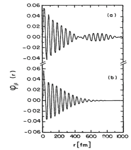
Figure 39: Radial wave functions for the discretized continuum using the histogram set (a) and the continuous set (b). From [BC92].

This set corresponds to histograms of constant height $1/\sqrt{\sigma}$ and width $\sigma$. The states $\Gamma_{j}(E)$ trivially satisfy the orthonormalization condition of Eq. (265). They present the advantage of leading to simple analytical expressions for the coupling matrix elements. On the other hand they have discontinuities at the edges, which lead to numerical difficulties. The second set consists of the functions

$$\chi_{j}(E)=N_{n_{j}}\;\left({\frac{E}{\sigma}}\right)^{n_{j}^{2}}\;e^{-n_{j}(E/\sigma)}.$$ (270)

The normalization constant

$$N_{n_{j}}={\frac{1}{\sqrt{\sigma}}}\;\left[{\frac{(2n_{j})^{2n_{j}^{2}+1}}{(2n_{j}^{2})!}}\right]^{1/2},$$ (271)

guarantees that $\int\chi_{j}(E)\,\chi_{j}(E)\,dE=1$. The functions $\chi_{j}$ are peaked at $E=n_{j}\,\sigma$ and have width $\approx\sigma$. The integer $n_{j}=K.j$ is proportional to the index-j and the proportionality constant, a small integer $K$, is a parameter of the set which determines the overlap of two consecutive functions $\chi_{j}$ and $\chi_{j+1}$. However, this set fails to satisfy the orthogonality condition of Eq. (268). This shortcoming can be fixed by the definition of a new set $\Gamma_{j}(E)$ of linear combinations

$$\Gamma_{j}(E)=\sum_{k=1}^{N}\,C_{jk}\,\chi_{k}(E),$$ (272)

with the coefficients $C_{ij}$ determined so that the resulting combinations be orthogonal. These coefficients can be found by means of an orthogonalization procedure as, e.g., the Gram-Schmidt method. The set of Eq. (272) has the advantages of being continuously derivable and of leading to reasonably simple coupling matrix elements.

A comparison between basis states $\phi_{j\ell m}(r)$ generated with each of these sets [through Eq. (264)] is made in Fig. 39. One observes that the discrete wavefunctions $\phi_{j\ell m}$ decrease rapidly enough with $r$, so that the matrix elements $<\phi_{j\ell m}|rY_{1\mu}|\phi_{j^{\prime}\ell^{\prime}m^{\prime}}>$ are finite. The use of the histograms (269) for $\Gamma_{j}(E)$ leads to beats in $\phi_{j\ell m}$ as displayed in Fig. 39(a). These beats are the result of the discontinuous nature of $\Gamma_{j}(E)$ and arise from the interference from the borders of the histograms. Due to this behavior, the numerical evaluation of $<\phi_{j\ell m}|rY_{1\mu}|\phi_{j^{\prime}\ell^{\prime}m^{\prime}}>$ is more involved than with the second set of $\Gamma_{j}$-functions, (272). Indeed, as we see from Fig. 39(b) the beats disappear with the use of the basis set (272). Although the use of plane-wave basis allows the derivation of simple results with both sets, this fact is of relevance for improved coupled-channels calculations in the continuum.

Using Eq. (264) and the properties of the spherical harmonics one finds

$$V_{j\ell m;j^{\prime}\ell^{\prime}m^{\prime}} = {\frac{(-1)^{m}}{\sqrt{2}}}\gamma Z_{T}e^{2}\left(Z_{c}\,{\frac{m_{b}}{m_{a}}}-Z_{b}\,{\frac{m_{c}}{m_{a}}}\right)$$ (273)

$$\times {\frac{\sqrt{(2\ell+1)(2\ell^{\prime}+1)}}{(b^{2}+\gamma^{2}v^{2}t^{2})^{3/2}}}\left({{\ell}\atop{0}}{{1}\atop{0}}{{\ell^{\prime}}\atop{0}}\right)$$

$$\times \Big{\{}ib\Big{[}\left({{\ell}\atop{-m}}{{1}\atop{1}}{{\ell^{\prime}}\atop{m^{\prime}}}\right)+\left({{\ell}\atop{-m}}{{1}\atop{-1}}{{\ell^{\prime}}\atop{m^{\prime}}}\right)\Big{]}$$

$$+ \sqrt{2}\,\gamma vt\left({{\ell}\atop{-m}}{{1}\atop{0}}{{\ell^{\prime}}\atop{m^{\prime}}}\right)\Big{\}}I_{j\ell;j\prime\ell\prime}$$

where

$$I_{j\ell;j^{\prime}\ell^{\prime}} = \int r^{3}dr\int dE\;\Gamma_{j}(E)\int dE^{\prime}\;\Gamma_{j^{\prime}}(E^{\prime})$$ (274)

$$\times u_{\ell,\,E}^{\ast}(r)u_{\ell^{\prime},\,E^{\prime}}(r).$$

From (273) one deduces that the interaction potential is different from zero only if $|\ell-\ell^{\prime}|=1$, as expected.

The use of the plane wave basis is especially useful because, exploiting the recursion and closure relations of the spherical Bessel functions, one obtains the general result

$$I_{j\ell;j^{\prime}\ell^{\prime}}={\frac{\hbar^{2}}{\mu}}\left\{{\frac{\ell+\ell^{\prime}+2}{2}}F_{jj^{\prime}}+\delta_{\ell,\ell^{\prime}+1}G_{j,j^{\prime}}+\delta_{\ell+1,\ell^{\prime}}G_{j^{\prime}j}\right\},$$ (275)

where

$$F_{jj^{\prime}} = \int dq\;\Gamma_{j}(E)\;\Gamma_{j^{\prime}}(E)$$

$$G_{jj^{\prime}} = \int dq\;q\;\Gamma_{j}(E)\;{\frac{d}{dq}}\Gamma_{j^{\prime}}(E)$$ (276)

with $E=\hbar^{2}q^{2}/2\mu$. Explicit forms can be found for each basis set:

(a) Histogram - Applying this relation to the histogram set (269), one can show that for $j,\;j^{\prime}\neq 0$

$$I_{j\ell;j^{\prime}\ell^{\prime}}=\hbar\sqrt{\frac{2}{\mu\sigma}}\left\{\begin{array}[]{l}{\frac{\ell+\ell^{\prime}+1}{2}}\;\left[\sqrt{j}-\sqrt{j-1}\right]\;\;\mathrm{if\;}\;j=j^{\prime}\\ -(-1)^{(j+\ell-j^{\prime}-\ell^{\prime})\over 2}\sqrt{\frac{j+j^{\prime}-1}{2}}\;\mathrm{if}\;|j-j^{\prime}|=1\\ 0\;\;\;\;\mathrm{otherwise.}\end{array}\right.\;$$ (277)

For $j=0$ or $j^{\prime}=0$, only the integral with $\ell$, or $\ell^{\prime}=1$ is necessary, and the result is

$$I_{00;\;j1}=I_{j1;\;00}={\frac{\sqrt{2\eta\sigma}}{\pi}}\;{\frac{E_{j}^{3/4}}{(E_{0}+E_{j})^{2}}}\;\left({\frac{\hbar^{2}}{2\mu}}\right)^{3/4}$$ (278)

where $E_{j}=(j-1/2)\,\sigma$.

(b) Continuous basis - For the set of continuous energy functions (272) one finds, for $j,\,j^{\prime}\neq 0$

$$\left\{\begin{array}[]{c}F_{jj^{\prime}}\\ G_{jj^{\prime}}\end{array}\right\} = \sqrt{\frac{\mu\sigma}{2\hbar^{2}}}\sum_{n,n^{\prime}}C_{jn}\,C_{j^{\prime}n^{\prime}}N_{n}\,N_{n^{\prime}}{\frac{\Gamma(n^{2}+n^{\prime}{}^{2}+1/2)}{(n+n^{\prime})^{n^{2}+n^{\prime}{}^{2}+1/2}}}$$ (281)

$$\times \left\{\begin{array}[]{c}1\\ 2n^{\prime}{}^{2}-\frac{n^{\prime}(2n^{2}+2n^{\prime}{}^{2}+1)}{n+n^{\prime}}\end{array}\right\}$$ (284)

where $\Gamma(z)$ is the gamma-function and we simplified the notation using $n\equiv n_{j}$. For $j=0$, or $j^{\prime}=0$, one finds

$$I_{00;\;j1} = I_{j1;\;00}={\frac{\sqrt{2\eta\sigma}}{\pi}}\;{\frac{E_{j}^{3/4}}{(E_{0}+E_{j})^{2}}}\;\left({\frac{\hbar^{2}}{2\mu}}\right)^{3/4}$$ (285)

$$\times \sum_{n}\,{\frac{n^{2}!}{n^{n^{2}+1}}}\;\sqrt{\frac{(2n)^{2n^{2}+1}}{(2n^{2})!}}\;C_{jn}\,.$$

Figure 40: (a) Radial matrix elements, Eqs. (273) and (274) for the transition $j\rightarrow j+1$ (dashed-line), and for the $j\rightarrow j$ one (solid line). We used $\ell=0$ and $\ell^{\prime}=1$. (b) Radial matrix elements for the transition $j\rightarrow j^{\prime}$, keeping $E_{j}=const.$ and varying $E_{j^{\prime}}$ [BC92].

As we have seen above, the use of the plane wave basis (266) results in the elegant derivation of $I_{j\ell;\;j^{\prime}\ell^{\prime}}$ presented by Eqs. (275) and (276). Nonetheless, the s-wave ($\ell=0$) state of Eq. (266) is not orthogonal to the bound-state wave function. To restore orthogonality one has to add an extra piece to this function. One expects however that this approximation does not affect the results appreciably since to access this state one needs at least two transitions: the $0\rightarrow j1$ followed by the $j^{\prime}1\rightarrow j^{\prime}0$ one. But the later transition competes with the transition to the ground state, $j1\rightarrow 00$, which is the dominant one. A more severe restriction is the use of plane waves to describe the continuum. A realistic calculation would have to use outgoing waves for $u_{\ell,\,E}^{(+)}(r)$ which would carry information about the final state interactions of the ($b+c$)-system.

The break-up probability per unit energy interval, $P_{(E)}^{BU}$, is given by

$$P_{(E)}^{BU}=\sum_{ij}\Gamma_{i}(E)\;\Gamma_{j}(E)\;Q_{ij}$$ (286)

where

$$Q_{ij}=\mathcal{R}e\;\left[\sum_{\ell m}a_{i\ell m}^{\ast}\,a_{j\ell m}\right]\,.$$ (287)

The validity of the dipole approximation for the interaction potential (273) to calculate the continuum-continuum coupling can only be justified for $qr\ll 1$. But, as shown in Fig. (39), the discretized wavefunctions extend up to $400\;$fm. Thus, unless the matrix elements for the continuum-continuum coupling, Eq. (274), have its main contribution from $r\ll 20$fm, the dipole approximation is not valid. The $jj$-coupling do satisfy this requirement. In this case the wave functions have equal energies, but different angular momenta. This causes an asymptotically ($r\gg 1/q$) constant phase difference between the wave functions entering in $I_{jl;jl^{\prime}}$. This leads to cancellations in the integrand of Eq. (274) for large $r$. The situation is different for the ($j,j^{\prime}\neq j$)-coupling. In this case the integrand has contributions from larger values of $r$ and these contributions increase with the energy. With a correct treatment of the multipole expansion of the interaction potential the integrals $I_{j\ell;j^{\prime}\neq j,\ell^{\prime}}$ would decrease with $E$. We expect that the transitions between $00\rightarrow j^{\prime},\ell=1$ and $j^{\prime},\ell=1\rightarrow 00$ dominate the excitation process, so that the matrix elements between states with $j\neq j^{\prime}\neq 0$ do not play an important role. Also, to minimize the consequence of the breaking down the dipole approximation in the continuum-continuum coupling at $j\neq j^{\prime}$, one can use a large parameter $K$ (e.g., here $K=4$ was used). This leads to small $I_{j\neq j^{\prime}}$.

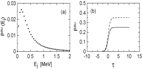
Figure 41: (a) Coulomb break-up probability, per unit energy interval (MeV^-1), of ¹¹Li projectiles incident on lead at 100 MeV/nucleon and $b=15\;$fm, as a function of the final total kinetic energy of the fragments. (b) Breakup probability as a function of the time, $\tau=vt/c$ [BC92].

In Figure 41(a) we show the break-up probability per unit energy interval for the reaction ${}^{11}\mathrm{Li}+\mathrm{Pb}$ at $100$ MeV/nucleon and $b=15\;$fm, calculated from Eq. (286) by solving the coupled-differential Eqs. (268) for $a_{i\ell m}$. We see that the energy distribution of the fragments is peaked at $E\sim 0.3\;$MeV. Therefore, the most relevant momentum transfer to the ¹¹Li nucleus occurs at $q=\sqrt{2\mu_{bc}B}/\hbar\sim 20\;$fm^-1.

In Figure 41(b) the solid line represents $P^{BU}$, the total breakup probability [Eq. (286) integrated over energy], as a function of the adimensional parameter $\tau=vt/b$, for $b=15\;$fm. This is obtained by solving the coupled-channels Eqs. (268) for a time $t$ and calculating the sum $P^{BU}(t)=\sum_{j\ell m}|a_{j\ell m}|^{2}$. The dashed-line corresponds to the neglect of all transitions, except for the $0\rightarrow j\ell$ ones. The solid-line includes all possible transitions. The break-up probability occurs in a time scale of $\Delta t\sim b/v$. As $t\rightarrow\infty$ the break-up probability is $40\%$ smaller than that calculated by first order perturbation theory.

IX.5.2 Dynamical model in space-time lattice

Another method for the treatment of higher-order effects in Coulomb breakup is the solution of the Schrödinger equation in a discretized space-time lattice [BB93,BB94,EBB95]. This should yield the same results as the CDCC model described in the previous section, if the model space is large enough. By that we mean that the wavefunction expansion in the CDCC method, and the lattice discretization in the present model, are robust, convergent, and accurate. With present computer power, this can only be achieved with rather simplified structure models.

One assumes a potential model for a cluster-like ($c+x$) halo nucleus. For example, a Woods-Saxon potential may be used for the nuclear interaction. To this potential a time-dependent non-relativistic Coulomb interaction is added,

$$V_{coul}=Z_{\tau}e^{2}[\frac{Z_{c}}{\mid\mathbf{r}_{c}-\mathbf{R}(t)\mid}+\frac{Z_{x}}{\mid\mathbf{r}_{x}-\mathbf{R}(t)\mid}-\frac{Z_{a}}{R(t)}]$$ (288)

where $\;a=c+x$  is the projectile, $\mathbf{r}_{c}=-\mathbf{r}A_{x}/A_{a}$, and $\mathbf{r}_{c}=\mathbf{r}(1-A_{x}/A_{a}).$

The potential above can be expanded into multipoles. Normally, the dipole part of the expansion is the most relevant one. The time dependent wavefunction for the relative motion of $c+x$ is given by

$$\Psi(\mathbf{r},t)=\frac{1}{r}\sum_{\ell m}u_{\ell m}(r,t)Y_{\ell m}(\widehat{\mathbf{r}}).$$ ((3.9) )

Inserting this expansion in the Schrödinger equation and retaining only the dipole expansion of the potential (288) we get

$$\left[\frac{d^{2}}{dr^{2}}-\frac{\ell(\ell+1)}{r^{2}}-\frac{2\mu_{cx}}{\hbar}V_{N}(r)\right]\;u_{\ell m}(r,t)$$ (289)

$$+ \sum\limits_{\ell^{\prime}m^{\prime}}S_{\ell^{\prime}m^{\prime}}^{(\ell m)}u_{\ell^{\prime}m^{\prime}}(r,t)=-\frac{2\mu_{cx}}{\hbar}\frac{\partial u_{\ell m}}{\partial t}$$

where

$$S_{\ell^{\prime}m^{\prime}}^{(\ell m)} = -\frac{2\mu_{cx}}{\hbar}\frac{(-1)^{m}}{\sqrt{2}}\left[b^{2}+v^{2}t^{2}\right]^{-3/2}$$ (292)

$$\times \sqrt{(2\ell+1)(2\ell^{\prime}+1)}\left(\begin{array}[]{lll}\ell&1&\ell^{\prime}\\ 0&0&0\end{array}\right)$$

$$\times \Bigg{\{}ib\left[\left(\begin{array}[]{lll}\ell&1&\ell^{\prime}\\ -m&1&-m^{\prime}\end{array}\right)+\left(\begin{array}[]{lll}\ell&1&\ell^{\prime}\\ -m&-1&-m^{\prime}\end{array}\right)\right]$$ (297)

$$+ \sqrt{2}vt\left(\begin{array}[]{lll}\ell&1&\ell^{\prime}\\ -m&0&-m^{\prime}\end{array}\right)\Bigg{\}}r.$$ (300)

This equation can be solved by a finite difference method. A truncation on the $\ell,m$ values is needed. Only a few angular momentum states are needed. Denoting $\alpha\equiv(\ell,m),$ the wave function $u_{\alpha}$ at time $t+\Delta t$ is obtained from the wave function at time $t$, according to the algorithm [BB93]

$$u_{\alpha}(t+\Delta t) = \left[\frac{1}{i\tau}-\Delta^{\left(2\right)}+\frac{\Delta t}{2\hbar\tau}V_{\alpha}\right]^{-1}$$

$$\times \left[\frac{1}{i\tau}+\Delta^{(2)}-\frac{\Delta t}{2\hbar\tau}V_{\alpha}+\frac{\Delta t}{\hbar\tau}\;\widehat{S}\right]u_{\alpha}(t).$$

In this equation $\tau=\hbar\Delta t/4\mu_{bx}(\Delta r)^{2}$ and $\widehat{S}u_{\alpha}(t)=\sum\limits_{\alpha^{\prime}}S_{\alpha^{\prime}}^{(\alpha)}u_{\alpha^{\prime}}(t).$ Also,

$$V_{\alpha}(r)=V_{N}(r)+\frac{\hbar^{2}\ell(\ell+1)}{2\mu_{bc}r^{2}}.$$ (303)

The wave functions $u_{\alpha}(r,t)$ are discretized in a mesh in space, with a mesh-size $\Delta r$. The second difference operator $\Delta^{(2)}$ is defined as

$$\Delta^{(2)}u_{\alpha}^{(j)}=u_{\alpha}^{(j+1)}(t)+u_{\alpha}^{(j-1)}(t)-2u_{\alpha}^{(j)}(t),$$

$$\text{with\ \ }u_{\alpha}^{(j)}\equiv u_{\alpha}(r_{j},t).$$ (304)

The 1^st operation on the right side of Eq. (LABEL:(3.12)) is trivial. The second one needs special attention (see Appendix H).

The wave function calculated numerically at a very large time will not be influenced by the Coulomb field. The numerical integration can be stopped there. The continuum part of the wave function is extracted by means of the relation (and normalized to unity)

$$\Psi_{c}(\mathbf{r},t) = \left[\Psi-\Psi_{gs}<\Psi_{gs}\mid\Psi>\right]$$ (305)

$$\times \left[1-\mid<\Psi_{gs}\mid\Psi>\mid^{2}\right]^{-1/2}$$

where $\Psi_{gs}$ is the initial wave function.

This wave function can be projected onto continuum eigenstates of the potential $V_{N}(r)$ in order to obtain the excitation probability of that state. For illustration lets us use the simplifying assumption that the final states are plane waves. A projection onto these states is equivalent to a Fourier transform of the time dependent wave function. One gets

$$\Psi_{c}(\mathbf{p)}=\sum\limits_{\ell m}C_{\ell m}(p)Y_{\ell m}(\widehat{\mathbf{p}})$$ (306)

where

$$C_{\ell m}(p)=\sqrt{\frac{2}{\pi}}\;i^{\ell}\;\int dr\;r\;j_{\ell}(pr)u_{\ell m}^{(c)}(r,t)$$ (307)

where $j_{\ell}$ is the spherical Bessel function. The probability density for an excitation to a final state with energy $E$ is

$$P(b,E,\Omega)=\frac{1}{2}\left(\frac{2\mu bx}{\hbar^{2}}\right)^{3/2}\sqrt{E}\mid\Psi_{c}(\widehat{\mathbf{p}})\mid^{2}.$$ (308)

Integrating over $\Omega$ :

$$P(b,E)=\frac{1}{2}\left(\frac{2\mu_{bx}}{\hbar^{2}}\right)^{3/2}\sqrt{E}\sum\limits_{\ell m}\mid C_{\ell m}(p)\mid^{2}.$$ (309)

In first-order perturbation theory this spectrum would be given by

$$P^{(1)}(b,E) = \frac{4\pi}{9}\left(\frac{2Z_{T}e^{2}}{\hbar v}\right)^{2}\left(\frac{E}{\hbar v}\right)^{2}\;\;\frac{dB(E1)}{dE}$$ (310)

$$\times \left[K_{0}^{2}(x)+K_{1}^{2}(x)\right]$$

where the $K^{\prime}s$ are the modified Bessel functions and $\;x=Eb/\hbar v.$ In this case $dB(E1)/dE$ is calculated by using the ground state and continuum states of the same potential for $c+x$.

As shown in figure 42, the first-order perturbation theory does not work well for the break-up of ¹¹Li at 28 MeV/nucleon.

Figure 42: (a) Energy spectrum for the breakup of ¹¹Li at 28 MeV/nucleon. Data points are from [Iek93]. Solid (dashed) line includes (does not include) the reacceleration effect [EBB95]. (b) Longitudinal relative momentum of the neutrons and the ⁹Li fragments in the breakup of ¹¹Li projectiles at 28 MeV/nucleon. Data are from Ref. [Iek93]. Solid curve is a calculation from Ref. [EBB95].

The reacceleration effect is very important in this case due to the very large break-up probabilities at small impact parameters. This induces higher order dynamical continuum-continuum interactions which distort the spectrum appreciably. One also observes that although the dynamical corrections modify the spectrum in the right direction the discrepancy with the experiment is appreciable. This might be a deficiency of the cluster model and has to be studied more carefully. Also, the spectrum of the relative longitudinal momentum of the fragments is not in a good agreement with the dynamical calculations of Ref. [EBB95], at least for the higher part of the spectrum. This is shown in the figure 42(b).

Higher-order effects are manifest in published theoretical calculations, and seem to have some experimental support. However, in most cases the effect is not relevant. There are also some theoretical results which does not show post-acceleration effects.

X Radiative capture in stars

If you have read to this point, you are now convinced that there must be numerous situations where Coulomb excitation and dissociation can be used for accessing precious information on nuclear structure. Obviously, any nucleus is part of a process in stars (perhaps the superheavies are not). Nuclear physics is therefore ultimately linked to astrophysics. We also expect that Coulomb dissociation plays a role in stars. In fact, it also plays a role in Cosmology. The Greisen-Zatsepin-Kuzmin (GZK) effect, for example, is nothing more that Coulomb excitation by (3 K) real photons remnant from the Big Bang and by virtual photons in intergalactic magnetic fields [GZK66].

As we have seen before, Coulomb excitation probes the same matrix elements as real photons. It is thus natural that many astrophysical reactions in stars involving photons in the initial or final channels can be studied on earth via Coulomb excitation. In particular, Coulomb dissociation is directly related to radiative capture in stars. In the next sections we discuss the Coulomb dissociation method, its experimental applications to some astrophysical problems and some of the newest theoretical developments and difficulties associated to it.

X.1 The Coulomb dissociation method

Coulomb dissociation is a process analogous to what happened to the comet Shoemaker-Levy as it disintegrated during its approximation to Jupiter in 1994 (see Figure 43). Approximately 1.5 to 2.2 hours after closest approach, the comet (which was presumably a single body at the time) was broken apart by tidal forces into at least 21 pieces. The pieces continued to orbit Jupiter with a period of approximately 2 years. Due to gravitational forces from the Sun, which changed the orbits slightly on the next approach to Jupiter, the pieces impacted the planet. Much stronger tidal forces occur when nuclei come close to each other due to their mutual electromagnetic field. This leads to their dissociation, especially for weakly-bound nuclei.

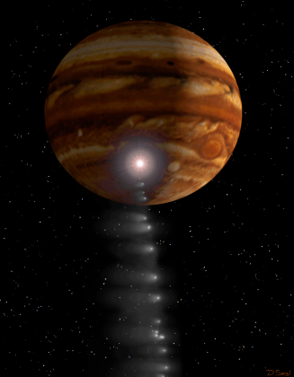
Figure 43: Jupiter and comet Shoemaker-Levy 9, as imaged by the Hubble Space Telescope (HST), on May 18, 1994, when the giant planet was at a distance of 420 million miles (670 million km) from Earth. The gravitational interaction of Jupiter with the comet has broken it up into many pieces (picture from NASA). Much stronger tidal forces occur when nuclei come close to each other due to their mutual electromagnetic fields.

The idea behind the Coulomb dissociation method is relatively simple. The (differential, or angle-integrated) Coulomb breakup cross section for $a+A\rightarrow b+c+A$ follows from

$${d\sigma_{C}^{\pi L}(E_{\gamma})\over d\Omega}=N^{\pi L}(E_{\gamma};\theta;\phi)\ .\ \sigma_{\gamma+a\ \rightarrow\ b+c}^{\pi L}(E_{\gamma}),$$ (311)

where $E_{\gamma}$ is the energy transferred from the relative motion to the breakup, and $\sigma_{\gamma+a\ \rightarrow\ b+c}^{\pi L}(E_{\gamma})$ is the photo-dissociation cross section for the multipolarity ${\pi L}$ and photon energy $E_{\gamma}$. Time reversal allows one to deduce the radiative capture cross section $b+c\rightarrow a+\gamma$ from $\sigma_{\gamma+a\ \rightarrow\ b+c}^{\pi L}(E_{\gamma})$, i.e.,

$$\sigma_{b+c\rightarrow\ \gamma+a}={2(2j_{a}+1)\over(2j_{b}+1)(2j_{c}+1)}{k_{\gamma}^{2}\over k^{2}}\sigma_{\gamma+a\ \rightarrow\ b+c},$$ (312)

where $k_{\gamma}=E_{\gamma}/\hbar c$ is the photon wavenumber, and $k=\sqrt{2\mu(E_{\gamma}-B)}/\hbar$ is the wavenumber for the relative motion of b+c. Except for the extreme case very close to the threshold ($k\rightarrow 0$), we have $k_{\gamma}\ll k$, so that the phase space favors the photodisintegration cross section as compared to the radiative capture. Direct measurements of the photodisintegration near the break-up threshold do hardly provide experimental advantages and seem presently impracticable. On the other hand the copious source of virtual photons acting on a fast charged nuclear projectile when passing the Coulomb field of a (large Z) nucleus offers a more promising way to study the photodisintegration process as Coulomb dissociation.

This method was introduced in Ref. [BBR86] and has been tested successfully in a number of reactions of interest to astrophysics. The most celebrated case is the reaction ⁷Be$(p,\gamma)^{8}$B, first studied in Ref. [Mot94], followed by numerous experiments in the last decade. This reaction is important because it produces ⁸B in the core of our sun. These nuclei decay by emitting a high energy neutrinos which are one of the best probes of the sun’s interior. The measurement of such neutrinos is very useful to test our theoretical solar models.

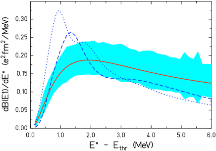
Figure 44: Electric dipole response function for ⁶He. The shaded area represents the experimental results from a Coulomb dissociation experiment [Aum99]. The dashed and dotted lines correspond to results from three-body decay models from Refs. [Da98,Cob97]. (Courtesy of T. Aumann).

Another example is the two-neutron capture on ⁴He could perhaps play a role in the post-collapse phase in type-II supernovae. The bottleneck in this nucleosynthesis scenario is the formation of nuclei with $A\geq 9$ from nucleons and $\alpha$-particles. In principle, the reaction ⁴He$(2n,\gamma)^{6}$He could be relevant in bridging the instability gap at $A=5$, although it is believed that this reaction cannot compete with the ($\alpha n,\gamma$) process in a type-II supernova scenario. Experiments with Coulomb dissociation have been used to study this question, as shown in the example presented in Figure 44. The figure displays the electric dipole response function for ⁶He. The shaded areas represent the experimental results from a Coulomb dissociation experiment [Aum99]. The dashed and dotted lines correspond to results from three-body decay models from Refs. [Dan98,Cob97].

In figure 45 we show the measurement of two-body correlations in the three-body decay of ⁶He. The lower panels display the ratio between the measured $\alpha$-n and $n$-$n$ relative-energy spectra (upper panels) and the spectra simulated (histograms) according to standard phasespace distributions [Aum99]. From the analysis of this experiment it was found that 10% of the dissociation cross section proceeds via the formation of ⁵He. A rough estimate yields 1.6 mb MeV for the photoabsorption cross section for ⁶He$(\gamma,n)^{5}$He, which agrees with theoretical calculations [Efr96]. From this experiment one concludes that the cross sections for formation of ⁵He and ⁶He via one (two) neutron capture by ⁴He are not large enough to compete with the ($\alpha$n, $\gamma$) capture process (for more details, see Ref. [Aum06]). Nonetheless, this and the previously mentioned examples, show the relevance of the Coulomb dissociation method to assess some of the basic questions of relevance for nuclear astrophysics.

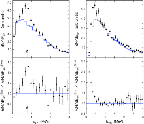
Figure 45: Measurement of two-body correlations in the three-body decay of ⁶He. The lower panels show the ratio between the measured $\alpha-n$ and $n$-$n$ relative-energy spectra (upper panels) and the spectra simulated (histograms) according to standard phasespace distributions [Aum99]. (Courtesy of T. Aumann).

X.2 Higher-order corrections

The Coulomb dissociation method is specially useful if first-order perturbation theory is valid. If not, one can still extract the electromagnetic matrix elements involved in radiative capture reactions. But a much more careful analysis of the high-order effects need to be done (see figure 46. We will discuss briefly a continuum-discretized coupled-channels calculation, appropriate for relativistic collision energies.

Coupled-channels calculations are a complication that we could live better without. It helps some people to get jobs, but they do not make life easier, as they have very often unphysical (or better said, unpredictable) results. The reason for the uncertain behavior is that, in each interaction step, plus and minus signs of matrix elements accumulate in one or the other direction (like a brownian motion). In seminars you might ask why a coupled-channels calculation reduced, or increased, the cross section. The plain answer is invariably: “it is a coupled-channels effect”. Well, who said that life is easy?

X.2.1 Continuum-Discretized Coupled-Channels

The continuum-discretized coupled-channels method (CDCC) [Kam87] is one of the most accurate models to describe the breakup of halo nuclei taking account of higher-order couplings explicitly. The eikonal CDCC method (E-CDCC) [Oga03,Oga06], is a derivation of CDCC that enables one to efficiently treat the nuclear and Coulomb breakup reactions at $E_{lab}\geq 50$ MeV/nucleon. An essential prescription described in Refs.  [Oga03,Oga06] is the construction of hybrid (quantum and eikonal) scattering amplitudes, with which one can make quantum-mechanical (QM) corrections to the pure eikonal wavefunctions with a minimum task. These corrections are, however, expected to become less important as the incident energy increases.

First I will describe a simplified CDCC method presented in Ref. Ber05] where the inclusion of relativistic continuum-continuum effects in CDCC calculations were introduced. Let us consider the Klein-Gordon (KG) equation with a potential $V_{0}$ which transforms as the time-like component of a four-vector [AC79]. For a system with total energy $E$ (including the rest mass $M$), the KG equation can be cast into the form of a Schrödinger equation (with $\hbar=c=1$),

$$\left(\nabla^{2}+k^{2}-U\right)\Psi=0,$$ (313)

where $k^{2}=\left(E^{2}-M^{2}\right)$ and $U=2V_{0}(2E-V_{0})$. When $V_{0}\ll M$, and $E\simeq M$, one gets $U=2MV_{0}$, as in the non-relativistic case. The condition $V_{0}\ll M$ is met in peripheral collisions between nuclei at all collision energies. Thus, one can always write $U=2EV_{0}$. A further simplification is to assume that the center of mass motion of the incoming projectile and outgoing fragments is only weakly modulated by the potential $V_{0}$.

To get the dynamical equations, one discretizes the wavefunction in terms of the longitudinal center-of-mass momentum $k_{z}$, using the ansatz

$$\Psi=\sum_{\alpha}\mathcal{S}_{\alpha}\left(z,\mathbf{b}\right)\ \exp\left(ik_{\alpha}z\right)\ \phi_{k_{\alpha}}\left(\mathbf{\mbox{\boldmath$\xi$}}\right).$$ (314)

In this equation, $\left(z,\mathbf{b}\right)$ is the projectile’s center-of-mass coordinate, with b equal to the impact parameter. $\ \phi\left(\mathbf{\mbox{\boldmath$\xi$}}\right)$ is the projectile intrinsic wavefunction and $\left(k,\mathbf{K}\right)$ is the projectile’s center-of mass momentum with longitudinal momentum $k$ and transverse momentum $\mathbf{K}$. There are hidden, uncomfortable, assumptions in Eq. (314). The center of mass of a relativistic system of interacting particles is not a well defined quantity. Also, the separation between the center of mass and intrinsic coordinates is not permissible under strict relativistic treatments. For high energy collisions we can at best justify Eq. (314) for the scattering of light projectiles on heavy targets. Eq. (314) is only reasonable if the projectile and target closely maintain their integrity during the collision, as in the case of very peripheral collisions.

Figure 46: Schematic description of a multi-step excitation, with excursions in the continuum.

Neglecting the internal structure means $\phi_{k_{\alpha}}\left(\mathbf{\mbox{\boldmath$\xi$}}\right)=1$ and the sum in Eq. (314) reduces to a single term with $\alpha=0$, the projectile remaining in its ground-state. It is straightforward to show that inserting Eq. (314) in the KG equation

$$\left(\nabla^{2}+k^{2}-2EV_{0}\right)\Psi=0,$$ (315)

and neglecting $\nabla^{2}\mathcal{S}_{0}\left(z,\mathbf{b}\right)$ relative to $ik\partial_{Z}\mathcal{S}_{0}\left(z,\mathbf{b}\right)$ one gets $ik\partial_{Z}\mathcal{S}_{0}\left(z,\mathbf{b}\right)=EV_{0}\mathcal{S}_{0}\left(z,\mathbf{b}\right)$, which leads to the center of mass scattering solution

$$\mathcal{S}_{0}\left(z,\mathbf{b}\right)=\exp\left[-iv^{-1}\int_{-\infty}^{z}dz^{\prime}\ V_{0}\left(z^{\prime},\mathbf{b}\right)\right],$$ (316)

with $v=k/E$. Using this result in the Lippmann-Schwinger equation, one gets the familiar result for the eikonal elastic scattering amplitude, i.e.

$$f_{0}=-i{k\over 2\pi}\int d\mathbf{b}\ \exp\left(i\mathbf{Q\cdot b}\right)\ \left\{\exp\left[i\chi(\mathbf{b})\right]-1\right\},$$

where the eikonal phase is given by $\chi(\mathbf{b})=\mathcal{S}_{0}\left(\infty,\mathbf{b}\right)$, and $\mathbf{Q}=\mathbf{K}^{\prime}-\mathbf{K}$ is the transverse momentum transfer.  Therefore, the elastic scattering amplitude in the eikonal approximation has the same form as that derived from the Schrödinger equation in the non-relativistic case.

For inelastic collisions we insert Eq. (314) in the KG equation and use the orthogonality of the intrinsic wavefunctions $\phi_{k_{\alpha}}\left(\mathbf{\mbox{\boldmath$\xi$}}\right)$. This leads to a set of coupled-channels equations for $\mathcal{S}_{\alpha}$:

$$\left(\nabla^{2}+k^{2}\right)\mathcal{S}_{\alpha}\mathrm{e}^{ik_{\alpha}z}=\sum_{\alpha}\left\langle\alpha\left|U\right|\alpha^{\prime}\right\rangle\ \mathcal{S}_{\alpha^{\prime}}\ \mathrm{e}^{ik_{\alpha^{\prime}}z},$$ (317)

with the notation $\left|\alpha\right\rangle=\left|\phi_{k_{\alpha}}\right\rangle$. Neglecting terms of the form $\nabla^{2}\mathcal{S}_{\alpha}\left(z,\mathbf{b}\right)$ relative to $ik\partial_{Z}\mathcal{S}_{\alpha}\left(z,\mathbf{b}\right)$, Eq. (317) reduces to

$$iv\frac{\partial\mathcal{S}_{\alpha}\left(z,\mathbf{b}\right)}{\partial z}=\sum_{\alpha^{\prime}}\left\langle\alpha\left|V_{0}\right|\alpha^{\prime}\right\rangle\ \mathcal{S}_{\alpha^{\prime}}\left(z,\mathbf{b}\right)\ \mathrm{e}^{i\left(k_{\alpha^{\prime}}-k_{\alpha}\right)z}.$$ (318)

The scattering amplitude for the transition $0\rightarrow\alpha$ is given by

$$f_{\alpha}\left(\mathbf{Q}\right)=-\frac{ik}{2\pi}\int d\mathbf{b}\ \ \exp\left(i\mathbf{Q\cdot b}\right)\ \left[S_{\alpha}\left(\mathbf{b}\right)-\delta_{\alpha,0}\right],$$ (319)

with $S_{\alpha}\left(\mathbf{b}\right)=\mathcal{S}_{\alpha}\left(z=\infty,\mathbf{b}\right)$. The set of equations (318) and (319) are the eikonal-CDCC equations (E-CDCC). They are much simpler to solve than the low-energy CDCC equations because the $z$ and $b$ coordinates decouple and only the evolution on the $z$ coordinate needs to be treated non-perturbatively.

The E-CDCC equations can be used to study the dissociation of ⁸B projectiles at high energies. The energies transferred to the projectile are small, so that the wavefunctions can be treated non-relativistically in the projectile frame of reference. In this frame the wavefunctions will be described in spherical coordinates, i.e. $\left|\alpha\right\rangle=\left|jlJM\right\rangle,$ where $j$, $l$, $J$ and $M$ denote the angular momentum numbers characterizing the projectile state. It is important to notice that the matrix element $\left\langle\alpha\left|V_{S}\right|\alpha^{\prime}\right\rangle$ is Lorentz invariant. Boosting a volume element from the projectile to the laboratory frame means $d^{3}\xi\rightarrow d^{3}\xi/\gamma$, where $\gamma=\left(1-v^{2}\right)^{-1/2}$ is the Lorentz contraction factor. The intrinsic projectile wavefunction is a scalar and transforms according to $\phi_{\alpha}\left(\xi_{x},\xi_{y},\xi_{z}\right)\rightarrow\phi_{\alpha}\left(\xi_{x},\xi_{y},\gamma\xi_{z}\right)$, while $V_{0}$, being the time-like component of a four-vector, transforms as $V_{0}\left(b,z;\xi_{x},\xi_{y},\xi_{z}\right)\rightarrow\gamma V_{0}\left(b,z;\xi_{x},\xi_{y},\gamma\xi_{z}\right)$. Thus, redefining the integration variable $z$ in the laboratory as $\mathbf{\xi}_{z}^{\prime}=\gamma\mathbf{\xi}_{z}$ leads to the afore mentioned invariance. We can therefore calculate $\left\langle\alpha\left|V_{0}\right|\alpha^{\prime}\right\rangle$ in the projectile frame.

The longitudinal wavenumber $k_{\alpha}\simeq(E^{2}-M^{2})^{1/2}$ also defines how much energy is gone into projectile excitation, since for small energy and momentum transfers $k_{\alpha}^{\prime}-k_{\alpha}=\left(E_{\alpha}^{\prime}-E_{\alpha}\right)/v$. In this limit, eqs. (318) and (319) reduce to semiclassical coupled-channels equations, if one uses $z=vt$ for a projectile moving along a straight-line classical trajectory, and changing to the notation $\mathcal{S}_{\alpha}\left(z,b\right)=a_{\alpha}(t,b)$, where $a_{\alpha}(t,b)$ is the time-dependent excitation amplitude for a collision wit impact parameter $b$. With these changes, equation (319) also agrees with the equivalent semiclassical equation for the inelastic scattering amplitude. Therefore, for non-relativistic collisions and small momentum and energy transfers, the above derivation reduces to previous methods used in the literature.

If the state $\left|\alpha\right\rangle$ is in the continuum (positive proton+⁷Be energy) the wavefunction is discretized according to

$$\left|\alpha;E_{\alpha}\right\rangle=\int dE_{\alpha}^{\prime}\ \Gamma(E_{\alpha}^{\prime})\ \left|\alpha;E_{\alpha}^{\prime}\right\rangle,$$ (320)

where the functions $\Gamma(E_{\alpha})$ are assumed to be strongly peaked around the energy $E_{\alpha}$ with width $\Delta E$. For convenience the histogram set is chosen. The inelastic cross section is obtained by solving the E-CDCC equations and using

$${d\sigma\over d\Omega dE_{\alpha}}=\left|f_{\alpha}\left(\mathbf{Q}\right)\right|^{2}\ \Gamma^{2}(E_{\alpha}).$$ (321)

The potential $V_{0}$ contains contributions from the nuclear and the Coulomb interaction. The nuclear potentials are constructed along traditional lines of non-relativistic theory. The potentials are also expanded into multipolarities. These potentials are then transformed as the time-like component of a four-vector, as described above. The multipole expansion of the Coulomb interaction in the projectile frame including retardation. The first term (monopole) of the expansion is the retarded Lienard-Wiechert potential which does not contribute to the excitation, but to the center of mass scattering. Due to its long range, it is hopeless to solve Eq. (318) with the Coulomb monopole potential, as $\mathcal{S}_{\alpha}\left(z,\mathbf{b}\right)$ will always diverge. This can be rectified by using the regularization scheme

$$S_{\alpha}\left(\mathbf{b}\right)\rightarrow\exp\left[i\left(2\eta\ln\left(kb\right)+\chi_{a}\left(b\right)\right)\right]\ S_{\alpha}\left(\mathbf{b}\right),$$ (322)

where $\eta=Z_{P}Z_{T}/\hbar v$ and the $S_{\alpha}\left(\mathbf{b}\right)$ on the right-hand side is now calculated without inclusion of the Coulomb monopole potential in Eq. (318). The purely imaginary absorption phase, $\chi_{a}\left(b\right)$, was introduced to account for absorption at small impact parameters.

The multipole-expansion of the relativistic Coulomb potential between the target nucleus (T) with the atomic number $Z_{\rm T}$ and the projectile (P), consisting of C and v clusters, are given in Ref. [Ber05]:

$$V_{{\rm E1}\mu}=\sqrt{\frac{2\pi}{3}}\xi Y_{1\mu}\left(\mathbf{\hat{\mbox{\boldmath$\xi$}}}\right)\frac{\gamma Z_{\rm T}ee_{\rm E1}}{\left(b^{2}+\gamma^{2}z^{2}\right)^{3/2}}\left\{\begin{array}[c]{c}\mp b\ \ (\mathrm{if}\ \ \ \mu=\pm 1)\\ \sqrt{2}z\ \ (\mathrm{if}\ \ \ \mu=0)\end{array}\right.$$ (323)

for the E1 (electric dipole) field and

$$V_{{\rm E2}\mu}= \sqrt{\frac{3\pi}{10}}\xi^{2}Y_{2\mu}\left(\mathbf{\hat{\mbox{\boldmath$\xi$}}}\right)\frac{\gamma Z_{\rm T}ee_{\rm E2}}{\left(b^{2}+\gamma^{2}z^{2}\right)^{5/2}}$$

$$\times\left\{\begin{array}[c]{c}b^{2}\ \ \ \ (\mathrm{if}\ \ \ \mu=\pm 2)\\ \mp 2\gamma^{2}bz\ \ \ \ (\mathrm{if}\ \ \ \mu=\pm 1)\\ \sqrt{2/3}\left(2\gamma^{2}z^{2}-b^{2}\right)\ \ \ \ (\mathrm{if}\ \ \ \mu=0)\end{array}\right.$$ (327)

for the E2 (electric quadrupole) field. In Eqs. (323)–(327), $e_{{\rm E}\lambda}=[Z_{\rm v}(A_{\rm C}/A_{\rm P})^{\lambda}+Z_{\rm C}(-A_{\rm v}/A_{\rm P})^{\lambda}]e$ are effective charges for $\lambda=1$ and 2 multipolarities for the breakup of ${\rm P}\rightarrow{\rm C}+{\rm v}$. The intrinsic coordinate of v with respect to C is denoted by $\xi$ and $b$ is the impact parameter (or transverse coordinate) in the collision of P and T, which is defined by $b=\sqrt{x^{2}+y^{2}}$ with ${\bf R}=(x,y,z)$, the relative coordinate of P from T in the Cartesian representation. Note that these relations are obtained with so-called far-field approximation [EB05], i.e. $R$ is assumed to be always larger than $\xi$. The Coulomb coupling potentials in E-CDCC are obtained with Eqs. (323)–(327) as shown below.

The full E-CDCC equations, including relativistic effects and recoil corrections for the three-body reaction are given by [OB09]:

$$\dfrac{i\hbar^{2}}{E_{c}}K_{c}^{(b)}(z)\dfrac{d}{dz}\psi_{c}^{(b)}(z) = \sum_{c^{\prime}}{\mathfrak{F}}^{(b)}_{cc^{\prime}}(z)\;{\cal R}^{(b)}_{cc^{\prime}}(z)$$ (328)

$$\times \psi_{c^{\prime}}^{(b)}(z)\ e^{i\left(K_{c^{\prime}}-K_{c}\right)z},$$

where $c$ denotes the channel indices {$i$, $\ell$, $m$}; $i>0$ ($i=0$) stands for the $i$th discretized-continuum (ground) state and $\ell$ and $m$ are respectively the orbital angular momentum between the constituents (C and v) of the projectile and its projection on the $z$-axis taken to be parallel to the incident beam. Note that we neglect the internal spins of C and v for simplicity. The impact parameter $b$ is relegated to a superscript since it is not a dynamical variable. The total energy and the asymptotic wave number of P are denoted by $E_{c}$ and $K_{c}$, respectively, and

$${\cal R}_{cc^{\prime}}^{(b)}(z)={(K_{c^{\prime}}R-K_{c^{\prime}}z)^{i\eta_{c^{\prime}}}\over(K_{c}R-K_{c}z)^{i\eta_{c}}}$$ (329)

with $\eta_{c}$ the Sommerfeld parameter. The local wave number $K_{c}^{(b)}(z)$ of P is defined by energy conservation as

$$E_{c}=\sqrt{(m_{\rm P}c^{2})^{2}+\left\{\hbar cK_{c}^{(b)}(z)\right\}^{2}}+\dfrac{Z_{\rm P}Z_{\rm T}e^{2}}{R},$$ (330)

where $m_{\rm P}$ is the mass of P and $Z_{\rm P}e$ ($Z_{\rm T}e$) is the charge of P (T). The reduced coupling-potential ${\mathfrak{F}}^{(b)}_{cc^{\prime}}(z)$ is given by

$${\mathfrak{F}}^{(b)}_{cc^{\prime}}(z)={\cal F}^{(b)}_{cc^{\prime}}(z)-\dfrac{Z_{\rm P}Z_{\rm T}e^{2}}{R}\delta_{cc^{\prime}},$$ (331)

where

$${\cal F}^{(b)}_{cc^{\prime}}(z)=\left\langle\Phi_{c}|U_{\rm CT}+U_{\rm vT}|\Phi_{c^{\prime}}\right\rangle_{\bf\xi}e^{-i(m^{\prime}-m)\phi_{R}}.$$ (332)

The $\Phi$ denotes the internal wave functions of P, $\phi_{R}$ is the azimuthal angle of ${\bf b}$ and $U_{\rm CT}$ ($U_{\rm vT}$) is the potential between C (v) and T consisting of nuclear and Coulomb parts. In actual calculations we use the multipole expansion ${\cal F}^{(b)}_{cc^{\prime}}(z)=\sum_{\lambda}{\cal F}^{\lambda(b)}_{cc^{\prime}}(z)$, the explicit form of which is shown in Ref. [Oga06].

In order to include the dynamical relativistic effects described above, we make the replacement

$${\cal F}^{\lambda(b)}_{cc^{\prime}}(z)\rightarrow\gamma f_{\lambda,m-m^{\prime}}{\cal F}^{\lambda(b)}_{cc^{\prime}}(\gamma z).$$ (333)

The factor $f_{\lambda,\mu}$ is set to unity for nuclear couplings, while for Coulomb couplings we take

$$f_{\lambda,\mu}=\left\{\begin{array}[]{cl}1/\gamma&\quad(\lambda=1,\mu=0)\\ \gamma&\quad(\lambda=2,\mu=\pm 1)\\ 1&\quad({\rm otherwise})\\ \end{array}\right.$$ (334)

following Eqs. (323) and (327). Correspondingly, we use

$$\dfrac{Z_{\rm P}Z_{\rm T}e^{2}}{R}\delta_{cc^{\prime}}\rightarrow\gamma\dfrac{Z_{\rm P}Z_{\rm T}e^{2}}{\sqrt{b^{2}+(\gamma z)^{2}}}\delta_{cc^{\prime}}$$ (335)

in Eqs. (330) and (331). The Lorentz contraction factor $\gamma$ may have channel-dependence, i.e., $\gamma=E_{c}/(m_{\rm P}c^{2})$, which we approximate by the value in the incident channel, i.e., $E_{0}/(m_{\rm P}c^{2})$.

It should be remarked that we neglect the recoil motion of T in Eq. (328); this can be justified because we consider reactions in which T is significantly heavier than P and we only treat forward-angle scattering in the present study [Ber05], as shown below. Note also that in the high incident-energy limit ${\cal R}_{cc^{\prime}}^{(b)}(z)\to 1$ and $K_{c}^{(b)}(z)\to K_{c}$, unless the energy transfer is extremely large. Thus, in this limit Eq. (328) becomes Lorentz covariant, as desired.

Using Eqs. (328)–(335), the dissociation observables in reactions of loosely bound nuclei ⁸B and ¹¹Be on ²⁰⁸Pb targets was calculated [OB09].

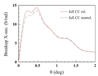
Figure 47: The total breakup cross section for ⁸B$+^{208}$Pb at 250 MeV/nucleon, as a function of the scattering angle of the c.m. of the projectile after breakup. The solid and dashed lines show the results of the full CC calculation with and without the dynamical relativistic effects, respectively.

Figure 47 shows the total breakup cross section of ⁸B by ²⁰⁸Pb at 250 MeV/nucleon, as a function of the scattering angle $\theta$ of the center-of-mass (c.m.) of the projectile after breakup. The solid and dashed lines represent the results of the E-CDCC calculation with and without the dynamical relativistic effects, respectively; in the latter we set $\gamma=1$ instead of the proper value 1.268 in Eqs. (333)–(335). Note that in all calculations shown in this work we use relativistic kinematics. One sees that the dynamical relativistic correction gives significantly larger breakup cross sections for $\theta<1.3$ degrees; the difference between the two around the peak is sizable, i.e. of the order of 10–15 %.

We show in Fig. 48 how the coupled-channel calculations affect the role of the dynamical relativistic correction. The left (right) panel corresponds to the calculation with both nuclear and Coulomb breakup (only Coulomb breakup).

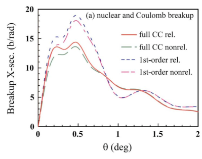
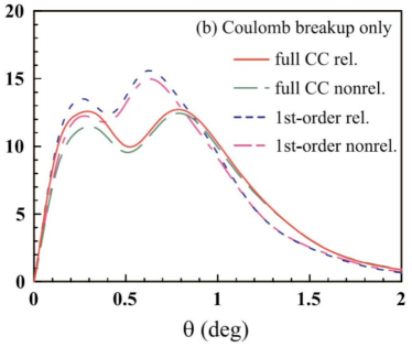
Figure 48: The total breakup cross sections for ⁸B$+^{208}$Pb at 250 MeV/nucleon with nuclear and Coulomb breakup (top panel) and only Coulomb breakup (bottom panel). The solid (dotted) and dashed (dash-dotted) lines show the results of the full CC (first-order perturbative) calculation with and without the relativistic correction, respectively.

In each panel the solid (dotted) and dashed (dash-dotted) lines show the results of the full CC (first-order perturbative) calculation with and without the dynamical relativistic correction, respectively. One sees from the left panel that relativistic corrections are slightly quenched when the first-order calculation is adopted. This is also the case when only Coulomb breakup is included, as shown in the right panel of Fig. 48. We stress here that due to continuum-continuum couplings relativistic effects are non-linear (and non-trivial to interpret). Thus, as shown in Fig. 48, one cannot infer the effect of relativistic corrections by simply carrying out first-order calculations. Moreover, it should be remarked that the full CC and first-order calculations give quite different breakup cross sections.

One concludes that the effects of relativistic corrections of the nuclear and Coulomb coupling potentials on the breakup cross sections of the weakly bound projectiles ⁸B and ¹¹Be by ²⁰⁸Pb targets at 250 and 100 MeV/nucleon. The relativistic corrections modify appreciably the breakup cross sections, at the level of 15 % (10%), in collisions at 250 (100) MeV/nucleon. This change is found to be due mainly to the modification of the Coulomb potential. We have also shown that relativistic corrections influence continuum-continuum transitions.

XI What you wanted to know, but were afraid to ask

XI.1 Close and far fields

So far, in all derivations of Coulomb excitation we restricted to distant collision, where the intrinsic radial coordinates are smaller than the minimum distance between the colliding nuclei. In calculations of the Coulomb dissociation of proton halo nuclei, it is of interest also to consider close collisions, since the density of the valence proton can extend to very large distances. Moreover, higher-order processes may also play a role, as suggested by the nonrelativistic calculations of the ⁸B breakup. This may be of relevance for the calculation of continuum-continuum matrix elements.

We derive a general expression for the multipole expansion of the electro-magnetic interaction from a fast charge particle, which can be employed in higher-order dynamical calculations of the Coulomb excitation of halo nuclei [EB05].

The relativistic expression for the electro-magnetic interaction from a fast charged particle, moving on a straight line trajectory in the z-direction and impact parameter b with respect to a target nucleus, i.e. ${\bf r}^{\prime}=(b,0,vt)$, and acting on a proton with coordinates ${\bf r}$ is

$$V_{\rm em}({\bf r},{\bf r}^{\prime})=Z_{T}e^{2}\Bigl{(}\phi-{{\bf v}\over 2mc^{2}}[\hat{\bf p}\phi+\phi\hat{\bf p}]\Bigr{)},$$ (336)

where $\phi$ is the Liénard-Wiechert potential

$$\phi={\gamma\over\sqrt{|{\bf b}-{\bf b}^{\prime}|^{2}+\gamma^{2}(z-z^{\prime})^{2}}},$$ (337)

and $\hat{\bf p}$ is the momentum operator associated with ${\bf r}$.

We start out with the Fourier representation of $\phi$ which can be written as (see appendix of Ref. [BB88])

$$\phi = {4\pi\over(2\pi)^{3}}\int d{\bf q}\ {e^{i{\bf q}\cdot({\bf r}-{\bf r}^{\prime})}\over q_{\perp}^{2}+q_{z}^{2}/\gamma^{2}}$$ (338)

$$= {4\pi\over(2\pi)^{3}}\int d{\bf q}\ {e^{i{\bf q}\cdot({\bf r}-{\bf r}^{\prime})}\over q^{2}}\ {1\over 1-\beta^{2}\ \cos^{2}(\theta_{q})}.$$

where $\beta=v/c$. Except for the last factor, this is just the ordinary Coulomb potential.

To proceed, we introduce the multipole expansion of the last term in Eq. (338) (see Eq. 8.825 of Ref. [GR80])

$${1\over 1-\beta^{2}\cos^{2}(\theta)}=\sum_{\lambda\ {\rm even}}(2\lambda+1)\ \beta^{-1}\ Q_{\lambda}(\beta^{-1})\ P_{\lambda}(\cos(\theta)),$$ (339)

and insert the plane wave expansion

$$e^{i{\bf q\cdot r}}=4\pi\sum_{LM}i^{L}\ j_{L}(qr)\ Y_{LM}^{*}({\hat{q}})Y_{LM}({\hat{r}})$$ (340)

for the two plane waves in Eq. (338). Thus we obtain

$$\phi=4\pi\sum_{LL^{\prime}}i^{L-L^{\prime}}\ R_{LL^{\prime}}(r,r^{\prime})\sum_{m}A_{lL^{\prime}M}(\beta)\ Y_{LM}({\hat{r}})\ Y_{L^{\prime}M}^{*}({\hat{r}}^{\prime}),$$ (341)

where

$$R_{LL^{\prime}}(r,r^{\prime}) = {2\over\pi}\int_{0}^{\infty}dq\ j_{L}(qr)\ j_{L^{\prime}}(qr^{\prime})$$

$$= {1\over\sqrt{rr^{\prime}}}\ \int_{0}^{\infty}{dq\over q}J_{L+1/2}(qr)\ J_{L^{\prime}+1/2}(qr^{\prime}),$$

and

$$A_{LL^{\prime}M}(\beta)=\langle Y_{LM}|{1\over 1-\beta^{2}\cos^{2}(\theta)}|Y_{L^{\prime}M}\rangle$$ (343)

$$=\sum_{\lambda\ {\rm even}}(2\lambda+1)\ \beta^{-1}Q_{\lambda}(\beta^{-1})\ \langle L^{\prime}M\lambda 0|LM\rangle\ \langle L0\lambda 0|L^{\prime}0\rangle.$$ (344)

The last two Clebsch-Gordan coefficients is the matrix element $\langle Y_{LM}|P_{\lambda}(\cos(\theta))|Y_{L^{\prime}M}\rangle.$

We note that different multipoles, $(LM)$ and $(L^{\prime}M)$, are mixed in the expansion (341). Let use therefore first take a look at the contribution from diagonal terms with $L^{\prime}=L$. Here the integral (XI.1) is particularly simple

$$R_{LL}(r,r^{\prime})={1\over 2L+1}\ {r_{<}^{L}\over r_{>}^{L+1}}$$ (345)

where $r_{<}=\min(r,r^{\prime})$ and $r_{>}=\max(r,r^{\prime})$. Inserting this into Eq. (341) we obtain the diagonal contribution

$$\phi_{\rm diag}=\sum_{L}{4\pi\over 2L+1}\ {r_{<}^{L}\over r_{>}^{L+1}}\sum_{m}A_{LLM}(\beta)\ Y_{LM}({\hat{r}})\ Y_{LM}^{*}({\hat{r}}^{\prime}).$$ (346)

This has a structure similar to the non-relativistic expression, except for the factor $A_{LLM}(\beta)$. In fact, in the non-relativistic limit we have $A_{LL^{\prime}M}(\beta=0)=\delta_{LL^{\prime}}$ and the non-relativistic expression is recovered.

The off-diagonal (i. e. $L^{\prime}\neq L$) contributions to $\phi$ are more complicated. According to Eq. (344), and the symmetry in $L$ and $L^{\prime}$, we only need expressions for $L^{\prime}=L+\Lambda$, $\Lambda=2,4,..$. One finds that [EB05]

$$R_{L,L+\Lambda}(a,b)=R_{L+\Lambda,L}(b,a)$$ (347)

$$R_{L,L+\Lambda}(a,b)=0,\ \ \ {\rm for}\ \ a\geq b,\ \ \ {\rm and}\ \ \Lambda=2,4,...$$ (348)

The explicit, non-zero expression is [EB05]

$$R_{L,L+\Lambda}(a,b)={1\over 2L+1+\Lambda}\ {a^{L}\over b^{L+1}}\ P_{\Lambda/2}^{(L+1/2,-1)}(1-2(a/b)^{2}),$$ (349)

which is valid when $a<b$, and $\Lambda=0,2,4,...$.

It is convenient to exploit the properties (347-348) and write expressions for $\phi$ that are valid for distant and close collisions, i. e. $r<r^{\prime}$ and $r>r^{\prime}$, respectively. The expression one obtains for distant collisions is

$$\phi_{\rm dist} = \sum_{LM}4\pi Y_{LM}({\hat{r}})\sum_{\Lambda=0,2,.}i^{\Lambda}\ R_{L,L+\Lambda}(r,r^{\prime})$$ (350)

$$\times A_{L,L+\Lambda,M}\ Y_{L+\Lambda,M}^{*}({\hat{r}}^{\prime}),$$

whereas the contribution for close collisions is

$$\phi_{\rm close} = \sum_{LM}4\pi Y_{LM}({\hat{r}})\sum_{\Lambda=0,2,.}i^{\Lambda}\ R_{L-\Lambda,L}(r^{\prime},r)$$ (351)

$$\times A_{L-\Lambda,L,m}\ Y_{L-\Lambda,L,m}^{*}({\hat{r}}^{\prime}).$$

The last sum over $\Lambda$ is finite since $L-\Lambda$ must be non-negative. The two expressions (350) and (351) reduce to Eq. (346) for $\Lambda=0$.

The above results have been recently used in Ref. [OB09b] to study the Coulomb breakup of ⁸B. It was concluded that the close field contributes very little to the breakup cross section. As there exists very few proton halo nuclei as loosely-bound as ⁸B, we conclude that the usual multipole expansion with distant fields describes Coulomb excitation satisfactorily.

XI.2 Comparison to electron scattering

In the plane wave Born approximation (PWBA) the cross section for inelastic electron scattering is given by [Ba62,EG88]

$$\frac{d\sigma}{d\Omega} =\frac{8\pi e^{2}}{\left(\hbar c\right)^{4}}\left(\frac{p^{\prime}}{p}\right)\sum_{L}\Bigg{\{}\frac{EE^{\prime}+c^{2}\mathbf{p\cdot p}^{\prime}+m^{2}c^{4}}{q^{4}}$$

$$\times\left|F_{ij}\left(q;CL\right)\right|^{2}$$

$$+\frac{EE^{\prime}-c^{2}\left(\mathbf{p\cdot q}\right)\left(\mathbf{p}^{\prime}\cdot\mathbf{q}\right)-m^{2}c^{4}}{c^{2}\left(q^{2}-q_{0}^{2}\right)^{2}}$$

$$\times\left[\left|F_{ij}\left(q;ML\right)\right|^{2}+\left|F_{ij}\left(q;EL\right)\right|^{2}\right]\Bigg{\}}$$ (352)

where $J_{i}$ $\left(J_{f}\right)$   is the initial (final) angular momentum of the nucleus, $\left(E,\mathbf{p}\right)$ and ($E^{\prime},\mathbf{p}^{\prime}$) are the initial and final energy and momentum of the electron, and $\left(q_{0},\mathbf{q}\right)=\left(\frac{(E-E^{\prime})}{\hbar c},\frac{\left(\mathbf{p-p}^{\prime}\right)}{\hbar}\right)$ is the energy and momentum transfer in the reaction. $F_{ij}\left(q;\Pi L\right)$ are form factors for momentum transfer $q$ and for Coulomb ($C$), electric ($E$) and magnetic ($M$) multipolarities, $\Pi=C,E,M$, respectively.

Here we will only treat electric multipole transitions. Moreover, we will treat low energy excitations such that $E,E^{\prime}\gg\hbar cq_{0}$, which is a good approximation for electron energies  $E\simeq 500$ MeV and small excitation energies $\Delta E=\hbar cq_{0}\simeq 1-10$ MeV. These are typical values involved in the dissociation of nuclei far from the stability line.

Using the Siegert’s theorem [Sie37,Sa51], one can show that the Coulomb and electric form factors in eq. (352) are proportional to each other. Moreover, for very forward scattering angles ($\theta\ll 1$) the PWBA cross section, eq. 352, can be rewritten as

$$\frac{d\sigma}{d\Omega dE_{\gamma}}=\sum_{L}\frac{dN_{e}^{(EL)}\left(E,E_{\gamma},\theta\right)}{d\Omega dE_{\gamma}}\ \sigma_{\gamma}^{(EL)}\left(E_{\gamma}\right),$$ (353)

where $\sigma_{\gamma}^{(EL)}\left(E_{\gamma}\right)$, with $E_{\gamma}=\hbar cq_{0}$, is the photo-nuclear cross section for the $EL$-multipolarity, given by eq. (105), which we rewrite as [BB88]

$$\sigma_{\gamma}^{(EL)}\left(E_{\gamma}\right)=\frac{\left(2\pi\right)^{3}\left(L+1\right)}{L\left[\left(2L+1\right)!!\right]^{2}}\left(\frac{E_{\gamma}}{\hbar c}\right)^{2L-1}\frac{dB\left(EL\right)}{dE_{\gamma}}.$$ (354)

In the long-wavelength approximation, the response function, $dB\left(EL\right)/dE_{\gamma},$ in eq. (354) is given by

$$\frac{dB\left(EL\right)}{dE_{\gamma}} = \frac{\left|\left\langle J_{f}\left\|Y_{L}\left(\widehat{\mathbf{r}}\right)\right\|J_{i}\right\rangle\right|^{2}}{2J_{i}+1}$$

$$\times \left[\int_{0}^{\infty}dr\ r^{2+L}\ \ \delta\rho_{if}^{\left(EL\right)}\left(r\right)\right]^{2}w\left(E_{\gamma}\right),$$

where $w\left(E_{\gamma}\right)$ is the density of final states (for nuclear excitations into the continuum) with energy $E_{\gamma}=E_{f}-E_{i}$. The the transition density $\delta\rho_{if}^{\left(EL\right)}\left(r\right)$ will depend upon the nuclear model adopted.

For $L\geq 1$ one obtains from Eq. (352) that

$$\frac{dN_{e}^{(EL)}\left(E,E_{\gamma},\theta\right)}{d\Omega dE_{\gamma}}=\frac{4L}{L+1}\frac{\alpha}{E}\left[\frac{2E}{E_{\gamma}}\sin\left(\frac{\theta}{2}\right)\right]^{2L-1}$$

$$\times\frac{\cos^{2}\left(\theta/2\right)\sin^{-3}\left(\theta/2\right)}{1+\left(2E/M_{A}c^{2}\right)\sin^{2}\left(\theta/2\right)}$$

$$\times\left[\frac{1}{2}+\left(\frac{2E}{E_{\gamma}}\right)^{2}\frac{L}{L+1}\sin^{2}\left(\frac{\theta}{2}\right)+\tan^{2}\left(\frac{\theta}{2}\right)\right].$$ (356)

One can also define a differential cross section integrated over angles. Since $\sigma_{\gamma}^{(EL)}$ does not depend on the scattering angle, this can be obtained from eq. (356) by integrating $dN_{e}^{(EL)}/d\Omega dE_{\gamma}$ over angles, from $\theta_{\min}=E_{\gamma}/E$ to a maximum value $\theta_{m}$, which depends upon the experimental setup.

Eqs. (353-356) show that under the conditions of the proposed electron-ion colliders, electron scattering will offer the same information as excitations induced by real photons. The reaction dynamics information is contained in the virtual photon spectrum of eq. (356), while the nuclear response dynamics information will be contained in Eq. (LABEL:photo3). This is akin to a method developed long time ago by Fermi [Fe24] and usually known as the Weizsaecker-Williams method [We34] (see section on historical note. The quantities $dN_{e}^{(EL)}/d\Omega dE_{\gamma}$ can be interpreted as the number of equivalent (real) photons incident on the nucleus per unit scattering angle $\Omega$ and per unit photon energy $E_{\gamma}.$ Note that $E0$ (monopole) transitions do not appear in this formalism. As immediately inferred from Eq. (LABEL:photo3), for $L=0$ the response function $dB\left(EL\right)/dE_{\gamma}$ vanishes because the volume integral of the transition density also vanishes in the long-wavelength approximation. But for larger scattering angles the Coulomb multipole matrix elements ($CL$) in Eq. (352) are in general larger than the electric ($EL$) multipoles, and monopole transitions become relevant [Sch54].

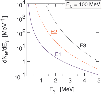
Figure 49: Virtual photon spectrum for the $E1$, $E2$ and $E3$ multipolarities in electron scattering off arbitrary nuclei at $E_{e}=100$ MeV and maximum scattering angle of 5 degrees.

In figure 49 we show the virtual photon spectrum for the $E1$, $E2$ and $E3$ multipolarities for electron scattering off arbitrary nuclei at $E_{e}=100$ MeV. These spectra have been obtained assuming a maximum scattering angle of 5 degrees. An evident feature deduced from this figure is that the spectrum increases rapidly with decreasing energies. Also, at excitation energies of 1 MeV, the spectrum yields the ratios $dN_{e}^{(E2)}/dN_{e}^{(E1)}\simeq 500$ and $dN_{e}^{(E3)}/dN_{e}^{(E2)}\simeq 100$. However, although $dN_{e}^{(EL)}/dE_{\gamma}$ increases with the multipolarity $L$, the nuclear response decreases rapidly with $L$, and $E1$ excitations tend to dominate the reaction. For larger electron energies the ratios $N^{(E2)}/N^{(E1)}$ and $N^{(E3)}/N^{(E1)}$ decrease rapidly.

In figure 50 we show a comparison between the $E1$ virtual photon spectrum, $dN_{e}/dE_{\gamma}$, of 1 GeV electrons with the spectrum generated by 1 GeV/nucleon heavy ion projectiles. In the case of Coulomb excitation, the virtual photon spectrum was calculated according to Eq. (LABEL:(A.6a)). For simplicity, we use for the strong interaction distance $R=10$ fm. The spectrum for the heavy ion case is much larger than that of the electron for large projectile charges. For ²⁰⁸Pb projectiles it can be of the order of 1000 times larger than that of an electron of the same energy. As a natural consequence, reaction rates for Coulomb excitation are larger than for electron excitation. But electrons have the advantage of being a cleaner electromagnetic probe, while Coulomb excitation at high energies needs a detailed theoretical analysis of the data due to contamination by nuclear excitation. As one observes in figure 50, the virtual spectrum for the electron contains more hard photons, i.e. the spectrum decreases slower with photon energy than the heavy ion photon spectrum. This is because, in both situations, the rate at which the spectrum decreases depends on the ratio of the projectile kinetic energy to its rest mass, $E/mc^{2},$ which is much larger for the electron ($m=m_{e}$) than for the heavy ion ($m=$ nuclear mass).

To obtain an effective luminosity per unit energy, the equivalent photon number is multiplied by the experimental luminosity, $L_{eA}$, i.e. $\frac{dL_{eff}}{dE_{\gamma}}=L_{eA}\frac{dN}{dE_{\gamma}}$. The number of events per unit time, $N_{\tau}$, is given by the integral $N_{\tau}=\int\sigma(E_{\gamma})dL_{eff}$, where $\sigma(E_{\gamma})$ is the photonuclear cross section. Assuming that the photonuclear cross section peaks at energy $E_{0}$ and using the Thomas-Reiche-Kuhn (TRK) sum rule, Eq. (206), we can approximate this integral by $N_{\tau}=\frac{dL_{eff}}{dE_{0}}\times 6\times 10^{-26}\frac{NZ}{A}$, where $dL_{eff}/dE$ is expressed in units of cm^-2s^-1MeV^-1. The giant resonances exhaust most part of the TRK sum rule and occur in nuclei at energies around $E_{0}=15$ MeV. For 1 GeV electrons $dN(E_{\gamma}=E_{0})/dE_{\gamma}\approx 6\times 10^{-3}$/MeV. With a luminosity of $L_{eA}=10^{25}$ cm^-2s^-1, one gets $\frac{dL_{eff}}{dE_{0}}\approx 6\times 10^{22}$ cm^-2MeV^-1s^-1 and a number of events $N_{\tau}\approx 4\times 10^{-3}NZ/A\approx 10^{-3}A$ s^-1. Thus, for medium mass nuclei, one expects thousands of events per day.

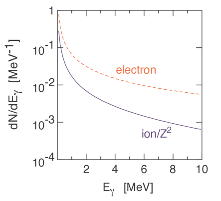
Figure 50: Comparison between the virtual photon spectrum of 1 GeV electrons (dashed line), and the spectrum generated by a 1 GeV/nucleon heavy ion projectile (solid line) for the $E1$ multipolarity, as a function of the photon energy. The virtual photon spectrum for the ion has been divided by the square of its charge number.

These estimates increase linearly with the accelerator luminosity, $L_{eA}$, and show that studies of giant resonances in neutron-rich nuclei is very promising at the proposed facilities [Haik05,Sud01]. Only a small fraction, of the order of 5%-10%, of the TRK sum-rule goes into the excitation of soft-dipole modes. However, these modes occur at a much lower energy, $E_{r}\approx 1$ MeV, where the number of equivalent photons (see figure 50) is at least one order of magnitude larger than for giant resonance energies. Therefore, inelastic processes leading to the excitation of soft dipole modes will be as abundant as those for excitation of giant resonances. However, one has to keep in mind that it is not clear if experiments with very short-lived nuclei will be feasible at the proposed electron-ion colliders.

XI.3 Non-inertial effects in Coulomb excitation

Extremely large accelerations occur when atomic nuclei collide. For instance, two lead nuclei in a head on collision with a center of mass kinetic energy of 500 MeV, reach a closest distance of 19.4 fm before they bounce back and move outward. At this distance each nucleus accelerates with an intriguing $\sim 10^{27}$ m/s². Very few other physical situations in the Universe involve nuclei undergoing such large accelerations, usually related to astrophysical objects, as in the vicinity of neutron stars and black holes, where huge gravitational fields exist. Here we will discuss the effects of large accelerations and large gravitational fields, and their possible influence on nuclear reactions in the laboratory and in astrophysical environments. Nuclear reactions are crucial for the formation of stellar structures and their rates could be affected by various factors.

There are two systems of reference which are often used to describe the effects of the collision: (a) the center-of-mass (cm) system of the two nuclei and (b) the system of reference of the excited nucleus. System (b) is appropriate to use when the intrinsic properties of the excited nucleus is described in some nuclear model. A typical example is the case of Coulomb excitation. One assumes that the nuclei scatter and their cm wave functions are described by Coulomb waves due to the Coulomb repulsion between the nuclei. Then one considers the residual effect of the Coulomb potential on the motion of the nucleons inside the nuclei. This is done by expanding the Coulomb potential in multipoles and using the high order terms (higher than first order) as a source of the excitation process. In this approach one illustrates the privileged role of the cm of the nuclear system: the net effect of the external forces is to (i) accelerate all the particles together, along with the cm of the system, and (ii) to change the intrinsic quantum state of the system through the spatial variation of the interaction within the system. Thus the theoretical treatment of accelerated many-body systems is well under control in non-relativistic dynamics.

In the non-relativistic case, the separation of variables into intrinsic motion and relative motion between the cm of each nucleus is a simple algebraic procedure. A problem arises when one wants to extend the method to describe intrinsic excitations of relativistic many-body systems. Very few works exist in the literature addressing this problem. The reason is that for nuclear reactions in the laboratory, the effect is expected to be very small, a common belief which must be tested. Another other reason is that in stellar environments where the gravitational fields are large, huge pressures develop, ”crushing” atoms, stripping them from their electrons, and ultimately making nuclei dissolve into their constituents. Effects of nuclear excitation are not relevant in the process.

Nuclei participating in nuclear reactions in a gaseous phase of a star follow inertial trajectories between collisions with other nuclei. Such trajectories are “free fall” trajectories in which all particles within the nucleus have the same acceleration. That is surely true in the non-relativistic case, but not in the relativistic one because retardation effects lead to corrections due to the nuclear sizes. The central problem here is the question regarding the definition of the center of mass of a relativistic many body system. We follow Refs. [LL89,Pry48,Few84], with few modifications, to show that a correction term proportional to the square of the acceleration appears in the frame of reference of the accelerated system. The results shown here are from Ref. [BHK09].

XI.3.1 Hamiltonian of an accelerated many-body system

Starting with a Lagrangian of a free particle in an inertial frame and introducing a coordinate transformation into an accelerated frame with acceleration $\mathcal{A}$, a “fictitious force” term appears in the Lagrangian when written in coordinates fixed to the accelerated frame. Thus, in an accelerated system the Lagrangian $L$ for a free particle can be augmented by a (non-relativistic) interaction term of the form $-m\mathcal{A}z$, that is

$$L=-mc^{2}+\frac{1}{2}mv^{2}-m\mathcal{A}z,$$ (357)

where $z$ is the particle’s coordinate along the direction of acceleration of the reference frame [LL89].

In the relativistic case, the first step to obtain the Lagrangian of a many body system in an accelerated frame is to setup an appropriate measure of space-time in the accelerated frame, i.e. one needs to find out the proper space-time metric. The free-particle action $S=-mc\int ds$ requires that $ds=(c-v^{2}/2c+{\cal A}z)dt$, which can be used to obtain $ds^{2}$. To lowest order in $1/c^{2}$ one gets

$$ds^{2}=c^{2}\left(1+\frac{\mathcal{A}z}{c^{2}}\right)^{2}dt^{2}-dx^{2}-dy^{2}-dz^{2}=g_{\mu\nu}d\xi^{\nu}d\xi^{\mu},$$ (358)

where ${\bf v}dt=d{\bf r}$ was used, with $d\xi^{\mu}=(cdt,dx,dy,dz)$ and $g_{\mu\nu}=\left(g_{00},-1,-1,-1\right)$, $g_{00}=\left(1+\mathcal{A}z/c^{2}\right)^{2}$. The indices $\mu$ run from $0$ to $3$. Eq. (358) gives a general form for the metric in an accelerated system. This approach can be found in standard textbooks (see, e.g. Ref. [LL89], $\S$ 87).

From the definition for the Hamiltonian, $H=\mathbf{p}\cdot\mathbf{v}-L$, with ${\bf p}=\partial L/\partial\mathbf{v}=m{\bf v}/\sqrt{g_{00}-v^{2}/c^{2}}$, and using the action with the metric of Eq. (358), after a straightforward algebra one finds

$$H=\frac{g_{00}mc^{2}}{\sqrt{g_{00}-\frac{v^{2}}{c^{2}}}}=c\sqrt{g_{00}\left(p^{2}+m^{2}c^{2}\right)}.$$ (359)

Expanding $H$ in powers of $1/c^{2}$, one obtains

$$H=\frac{p^{2}}{2m}\left(1-\frac{p^{2}}{4m^{2}c^{2}}\right)+m\mathcal{A}z\left(1+\frac{p^{2}}{2m^{2}c^{2}}\right)+\mathcal{O}\left({1\over c^{4}}\right).$$ (360)

This Hamiltonian can be applied to describe a system of particles with respect to a system of reference moving with acceleration $\mathcal{A}$, up to order $1/c^{2}$. For an accelerated nucleus the obvious choice is the cm system of the nucleus. But then the term carrying the acceleration correction averages out to zero in the center of mass, as one has ($\sum_{i}m_{i}\mathcal{A}z_{i}=0$). There is an additional small contribution of the acceleration due to the term proportional to $p^{2}$. Instead of exploring the physics of this term, one has to account for one more correction as explained below.

The above derivation of the Hamiltonian for particles in accelerated frames does not take into account that the definition of the cm of a collection of particles is also modified by relativity. This is not a simple task as might seem at first look. There is no consensus in the literature about the definition of the cm of a system of relativistic particles. The obvious reason is the role of simultaneity and retardation. Ref. [Pry48] examines several possibilities. For a system of particles it is found convenient to define the coordinates $q^{\mu}$ of the center of mass as the mean of coordinates of all particles weighted with their dynamical masses (energies). The relativistic (covariant) generalization of center of mass is such that the coordinates $q^{\mu}$ must satisfy the relation [Pry48]

$$P^{0}q^{\mu}={\displaystyle\sum\limits_{i}}p_{i}^{0}z_{i}^{\mu},$$ (361)

where the coordinates of the ith particle with respect to the center of mass are denoted by $z_{i}^{\mu}$ and the total momentum vector by $P^{\mu}={\displaystyle\sum\limits_{i}}p_{i}^{\mu}$. Ref. [Pry48] chooses eq. (361) as the one that is most qualified to represent the definition of cm of a relativistic system, which also reduces to the non-relativistic definition of the center of mass. We did not find a better discussion of this in the literature and we could also not find a better way to improve on this definition.

The above definition, Eq. (361), leads to the compact form, to order $1/c^{2}$,

$${\displaystyle\sum\limits_{i}}\frac{m_{i}\mathbf{r}_{i}}{\sqrt{g_{00}-\frac{v_{i}^{2}}{c^{2}}}} = {\displaystyle\sum\limits_{i}}m_{i}\mathbf{r}_{i}\left(1+\frac{v_{i}^{2}}{2c^{2}}-\frac{z_{i}\mathcal{A}}{c^{2}}+\mathcal{O}({1\over c^{4}})\right)$$ (362)

$$= 0,$$

where $\mathbf{r}_{i}=(x_{i},y_{i},z_{i})$ is the coordinate and $v_{i}$ is the velocity of the ith particle with respect to the cm.

For a system of non-interacting particles the condition in Eq. (362) implies that, along the direction of motion,

$${\displaystyle\sum\limits_{i}}\mathcal{A}m_{i}z_{i}=-{\displaystyle\sum\limits_{i}}\mathcal{A}m_{i}z_{i}\left(\frac{v_{i}^{2}}{2c^{2}}-\frac{z_{i}\mathcal{A}}{c^{2}}\right).$$ (363)

Hence, the Hamiltonian of Eq. (360) for a collection of particles becomes

$$H={\displaystyle\sum\limits_{i}}\frac{p_{i}^{2}}{2m_{i}}\left(1-\frac{p_{i}^{2}}{4m_{i}^{2}c^{2}}\right)+\frac{\mathcal{A}^{2}}{c^{2}}{\displaystyle\sum\limits_{i}}m_{i}z_{i}^{2}+U\left(r_{i}\right)+\mathcal{O}({1\over c^{4}}),$$ (364)

where we have added a scalar potential $U\left(r_{i}\right)$, which would represent a (central) potential within an atom, a nucleus, or any other many-body system.

Notice that the term proportional to $-m\mathcal{A}z$ completely disappears from the Hamiltonian after the relativistic treatment of the cm. This was also shown in Ref. [Few84]. It is important to realize that non-inertial effects will also carry modifications on the interaction between the particles. For example, if the particles are charged, there will be relativistic corrections (magnetic interactions) which need to be added to the scalar potential $U\left(r_{i}\right)=\sum_{j\neq i}Q_{i}Q_{j}/\left|\mathbf{r}_{i}-\mathbf{r}_{j}\right|$. As shown in Ref. [Few84], the full treatment of non-inertial effects together with relativistic corrections will introduce additional terms proportional to $\mathcal{A}$ and $\mathcal{A}^{2}$ in the Hamiltonian of Eq. (364), to order $1/c^{2}$. Thus, a more detailed account of non-inertial corrections of a many-body system requires the inclusion of $\mathcal{A}$-corrections in the interaction terms, too. We refer the reader to Ref. [Few84] where this is discussed in more details. Here we will only consider the consequences of the acceleration correction term in Eq. (364),

$$H_{nin}=\frac{\mathcal{A}^{2}}{c^{2}}{\displaystyle\sum\limits_{i}}m_{i}z_{i}^{2}.$$ (365)

XI.3.2 Reactions in the laboratory

For a nuclear fusion reaction, at the Coulomb radius (distance of closest approach, $R_{C}$) the nuclear acceleration is given by

$$\mathcal{A}_{C}={Z_{1}Z_{2}e^{2}\over R_{C}^{2}m_{0}},$$ (366)

where $m_{0}=m_{N}A_{1}A_{2}/\left(A_{1}+A_{2}\right)$ is the reduced mass of the system and $m_{N}$ is the nucleon mass. For typical values, $E=1$ MeV, $Z_{1}=Z_{2}=10$, and $A_{1}=A_{2}=20$, one obtains $R_{C}=Z_{1}Z_{2}e^{2}/E=144$ fm and $\mathcal{A}_{C}=6.2\times 10^{25}$ m/s². This is the acceleration that the cm of each nucleus would have with respect to the laboratory system.

The c.m. of the excited nucleus is the natural choice for the reference frame. This is because it is easier to adopt a description of atomic and nuclear properties in the cm frame of reference. Instead, one could also chose the cm of the colliding particles. This later (inertial) system makes it harder to access the acceleration effects, as one would have to boost the wave functions to an accelerated system, after calculating it in the inertial frame. This is a more difficult task. Therefore we adopt the cm reference frame of the excited nucleus, using the Hamiltonian of the previous section. This Hamiltonian was deduced for a constant acceleration. If the acceleration is time-dependent, the metric of Eq. (358) also changes. Thus, in the best case scenario, the Hamiltonian of Eq. (364) can be justified in an adiabatic situation in which the relative velocity between the many-body systems is much smaller than the velocity of their constituent particles with respect to their individual center of masses.

XI.3.3 Reactions involving halo nuclei

The nuclear wave-function of a (s-wave) loosely-bound, or “halo”, state can be conveniently parameterized by

$$\Psi\simeq\sqrt{\alpha\over 2\pi}\ {\exp\left(-\alpha r\right)\over r},$$ (367)

where the variable $\alpha$ is related to the nucleon separation energy through $S=\hbar^{2}\alpha^{2}/2m_{N}$. In first order perturbation theory the energy shift of a halo state will be given by

$$\Delta E_{nin}^{N}=\left\langle\Psi\left|H_{nin}\right|\Psi\right\rangle={1\over 8S}{\left(Z_{1}Z_{2}e^{2}\hbar\over R_{C}^{2}m_{0}c\right)^{2}}.$$ (368)

Assuming a small separation energy $S=100$ keV, and using the same numbers in the paragraph after Eq. (366), we get $\Delta E_{nin}^{N}=0.024$ eV, which is very small, except for states very close to the nuclear threshold, i.e. for $S\rightarrow 0$. But the effect increases with $Z^{2}$ for symmetric systems (i.e. $Z_{1}=Z_{2}=A_{1}/2$). It is thus of the order of $\Delta E_{nin}^{N}=1-10$ eV for larger nuclear systems.

There might exist situations where this effect could be present. For instance, the triple-alpha reaction which bridges the mass = 8 gap and forms carbon nuclei in stars relies on the lifetime of only 10^-17 s of ⁸Be nuclei. It is during this time that another alpha-particle meets ⁸Be nuclei in stars leading to the formation of carbon nuclei. This lifetime corresponds to an energy width of only $5.57\pm 0.25$ eV [Ti04]. As the third alpha particle approaches ⁸Be, the effects of linear acceleration will be felt in the reference frame of ⁸Be. This will likely broaden the width of the ⁸Be resonance (which peaks at $E_{R}=91.84\pm 0.04$ KeV) and consequently its lifetime. However, this line of thought could be wrong if one assumes that the third alpha particle interacts individually with each of the two alpha particles inside ⁸Be, and that the effects of acceleration internal to the ⁸Be nucleus arise from the different distances (and thus accelerations) between the third alpha and each of the first two. This effect has not been discussed elsewhere and deserves further investigation, if not for this particular reaction maybe for other reactions of astrophysical interest involving very shallow nuclear states.

XI.3.4 Nuclear transitions

Many reactions of astrophysical interest are deduced from experimental data on nucleus-nucleus scattering. Important information on the position and widths of resonances, spectroscopic factors, and numerous other quantities needed as an input for reaction network calculations in stellar modeling are obtained by the means of nuclear spectroscopy using nuclear collisions in the laboratory. During the collision the nuclei undergo huge acceleration, of the order of $\mathcal{A}\simeq 10^{28}$ m/s². Hence, non-inertial effects will be definitely important.

A simple proof of the statements above can be obtained by studying the Coulomb excitation. The simplest treatment that one can use in the problem is a semi-classical calculation. Following the same procedure leading to Eq. (58), we can calculate the contribution of the Hamiltonian of Eq. (365). In this case, ${\cal A}=Z_{1}Z_{2}e^{2}/m_{0}r^{2}$ and the pertubative potential $\phi=V_{nin}$ is given by

$$V_{nin}=\left({Z_{1}Z_{2}e^{2}\over m_{0}}\right)^{2}{Xm_{N}\over c^{2}r^{4}},$$ (369)

where we assume that $X$ nucleons participates in the transition. One then finds

$$a_{if}^{nin}=\left({Z_{1}Z_{2}e^{2}\over m_{0}}\right)^{2}{32Xm_{N}Q_{if}\over 15is^{3}\hbar v_{0}c^{2}}.$$ (370)

The ratio between the two transition probabilities (the above one and Eq. (58)) is

$$\left|{a_{if}^{nin}\over a_{if}}\right|^{2}=\left(8Xm_{N}Z_{1}Z_{2}^{2}e^{2}\over 5sm_{0}^{2}c^{2}\right)^{2}.$$ (371)

Applying Eq. (371) to the lead-lead collision at 500 MeV, we find $\left|{a_{if}^{nin}/a_{if}}\right|^{2}=(0.0093X)^{2}$. This yields very small results for the effect of non-inertial effects in single particle transitions ($X\simeq 1$), but can become appreciable for the excitation of collective states such as the giant resonances, for which $X\gg 1$.

XII Codes

GOSIA -

A non-relativistic semiclassical coupled-channel Coulomb excitation least-squares search code, GOSIA, has been developed to analyze the large sets of experimental data. Manual and code available from:

http://www.pas.rochester.edu/ cline/Gosia/

DWEIKO -

A relativistic coupled-channels code for Coulomb and nuclear excitations of E1, E2, E3,M1, and M2 multipolarities.

Manual: C.A. Bertulani, C.M. Campbell, T. Glasmacher, Computer Physics Communications 152 (2003) 317.

Code available from the Computer Physics Communications Program Library:

http://www.cpc.cs.qub.ac.uk/cpc/

COULINT -

A code which incorporates retardation corrections and recoil at intermediate energy collisions ($\sim 100$ MeV/nucleon), appropriate for Coulomb excitation at rare isotopes facilities, such as GANIL, GSI, NSCL and RIKEN. Under development. Preliminary versions already available [Ber04].

XIII Appendices

Here I discuss a few of the basic principles of quantum mechanics which are necessary to understand this review.

XIII.1 Decay rates

A quantum system, described by a wavefunction that is an Hamiltonian eigenfunction, is in a well defined energy state and, if it does not suffer external influences, it will remain indefinitely in that state. But this ideal situation does not prevail in excited nuclei, or in the ground state of an unstable nuclei. Interactions of several types can add a perturbation to the Hamiltonian and the pure energy eigenstates no more exist. In this situation a transition to a lower energy level of the same or of another nucleus can occur.

An unstable state normally lives a long time compared to the fastest nuclear processes, e. g., the time spent by a particle with velocity near that of the light to cross a nuclear diameter. In this way we can admit that a nuclear state is approximately stationary, and to write for its wave function:

$$\Psi(\mathbf{r},t)=\psi(\mathbf{r})e^{-iWt/\hbar}.$$ (372)

$|\Psi(\mathbf{r},t)|^{2}dV$ is the probability to find the nucleus in the volume $dV$ and, if the state described by $\Psi$ decays with a decay constant $\lambda$, it is reasonable to write

$$|\Psi(\mathbf{r},t)|^{2}=|\Psi(\mathbf{r},0)|^{2}e^{-\lambda t}.$$ (373)

To obey simultaneously (372) and (373), $W$ must be a complex quantity with imaginary part $-\lambda\hbar/2$. We can write:

$$W=E_{0}-{\frac{\hbar\lambda}{2}}i,$$ (374)

which shows that the wave function (372) does not represent a well defined stationary state since the exponential contains a real part $-\lambda t/2$. However, we can write the exponent of (372) as a superposition of values corresponding to well defined energies $E$ (for $t\geq 0$):

$$e^{-(iE_{0}/\hbar+\lambda/2)t}=\int_{-\infty}^{+\infty}A(E)e^{-iEt/\hbar}\,dE.$$ (375)

Functions connected by a Fourier transform relate to each other as

$$f(t) ={\frac{1}{\sqrt{2\pi}}}\int_{-\infty}^{+\infty}g(\omega)e^{-i\omega t}\,d\omega,$$ (376)

$$g(\omega) ={\frac{1}{\sqrt{2\pi}}}\int_{-\infty}^{+\infty}f(t)e^{i\omega t}\,dt.$$ (377)

This allows to establish the form of the amplitude $A(E)$:

$$A(E)={\frac{1}{2\pi\hbar}}\int_{0}^{+\infty}e^{[i(E-E_{0})/\hbar-\lambda/2]t}\,dt,$$ (378)

where the lower limit indicates that the stationary sate was created at the time $t=0$. The integral (378) is of easy solution, giving

$$A(E)={\frac{1}{h\lambda/2-2\pi i(E-E_{0})}}.$$ (379)

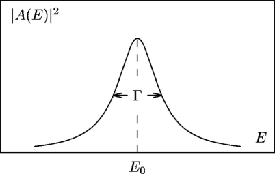
Figure 51: Form of the distribution (380).

The probability of finding a value between $E$ and $E+dE$ in an energy measurement is given by the product

$$A^{\ast}(E)A(E)={\frac{1}{h^{2}\lambda^{2}/4+4\pi^{2}(E-E_{0})^{2}}},$$ (380)

and this function of energy has the form of a Lorentzian, with the aspect shown in figure 51. Its width at half-maximum is $\Gamma=\hbar\lambda=\hbar/\tau$. The relationship

$$\tau\Gamma=\hbar$$ (381)

between the half-life and the width of a state is directly connected to the uncertainty principle and shows that the longer time a state survives the greater is the precision with which its energy can be determined. In particular, only to stable states one can attribute a single value for the energy.

The decay constant $\lambda$ was presented as the probability per unit time of occurrence of a transition between quantum states, and its values were supposed to be known experimental data. Now we will show that a formula to evaluate the decay constant can be obtained from the postulates of perturbation theory.

XIII.2 Coupled-channels

We can describe an unstable state by the addition of a perturbation to a stationary state. Formally we can write

$$H=H_{0}+V,$$ (382)

where $H$ is the Hamiltonian of the unstable state, composed by the non-perturbed Hamiltonian $H_{0}$ and a small perturbation $V$. The Hamiltonian $H_{0}$ satisfies an eigenvalue equation

$$H_{0}\psi_{n}=E_{n}\psi_{n},$$ (383)

whose eigenfunctions form a complete basis in which the total wavefunction $\Psi$, that obeys

$$H\Psi=i\hbar\frac{\partial\Psi}{\partial t},$$ (384)

can be expanded:

$$\Psi=\sum_{n}a_{n}(t)\psi_{n}e^{-iE_{n}t/\hbar}.$$ (385)

Using (382) and (385) in (384), and with the aid of (383), we obtain:

$$i\hbar\sum_{n}\dot{a}_{n}\psi_{n}e^{-iE_{n}t/\hbar}=\sum_{n}Va_{n}\psi_{n}e^{-iE_{n}t/\hbar},$$ (386)

with $\dot{a}_{n}\equiv\partial a_{n}(t)/\partial t$. Using the orthogonalization properties of the $\psi_{n}$, let us multiply (386) by $\psi_{k}^{\ast}$ and integrate it in the coordinate space. From this, results the coupled-channels equations

$$\dot{a}_{k}\left(t\right)=-\frac{i}{\hbar}\sum_{n}a_{n}\left(t\right)\ V_{kn}\left(t\right)\ e^{i{\frac{E_{k}-E_{n}}{\hbar}}t},$$ (387)

where we introduced the matrix element ($d\tau$ is the volume element)

$$V_{kn}=\int\psi_{k}^{\ast}V\psi_{n}\,d\tau.$$ (388)

XIII.3 Transition rates and cross sections

Let us make the following assumptions about the perturbation $V$: it begins to act at time $t=0$, when the unperturbed system is described by an eigenstate $\psi_{m}$. It stays at a very low value and after a short time interval becomes zero at $t=T$. These assumptions allow us to say that the conditions

$$a_{m}=1,\ \ \ \ \ \ \ \ \ \ \ \ \ \text{and}\ \ \ \ \ \ a_{m}=0\;\;\;\;\;\text{if}\;\;\;(m\neq n)$$ (389)

are rigorously verified for $t<0$ and also works approximately for $t>0$. Thus, (387) has only one term and the value of the amplitude is obtained from

$$a_{k}=-\frac{i}{\hbar}\int_{0}^{T}V_{km}e^{i\left(E_{k}-E_{m}\right)t/\hbar}\,dt,$$ (390)

whose value must be necessarily small by the assumption that followed (389). The above approach is also known as first order perturbation theory. The integral of (390) gives

$$a_{k}=\frac{V_{km}\left[1-\exp\left(i\frac{E_{k}-E_{m}}{\hbar}T\right)\right]}{E_{k}-E_{m}}.$$ (391)

We need now to interpret the meaning of the amplitude $a_{k}$. The quantity $a_{k}^{\ast}a_{k}$ measures the probability of finding the system in the state $k$. This characterizes a transition occurring from the initial state $m$ to the state $k$, and the value of $a_{k}^{\ast}a_{k}$ divided by the interval $T$ should be a measure of the decay constant $\lambda_{k}$ relative to the state $k$. The total decay constant is obtained by the sum over all states:

$$\lambda=\sum_{k\neq m}L_{k}=\frac{\sum|a_{k}|^{2}}{T}.$$ (392)

Let us now suppose that there is a large number of available states $k$. We can in this case replace the summation in (392) by an integral. Defining $\rho(E)$ as the density of available states around the energy $E_{k}$, we write

$$\lambda = \frac{1}{T}\int_{-\infty}^{+\infty}|a_{k}|^{2}\rho(E_{k})\,dE_{k}$$

$$= \frac{4}{T}\int_{-\infty}^{+\infty}|V_{km}|^{2}\frac{\sin^{2}[\left[\left({\frac{E_{k}-E_{m}}{2\hbar}}\right)T\right]}{(E_{k}-E_{m})^{2}}\rho(E_{k})\,dE_{k}.$$

The function sin${}^{2}x/x^{2}$ only has significant amplitude near the origin. In the case of (LABEL:5.49), if we suppose that $V_{km}$ and $\rho$ do not vary strongly in a small interval of the energy $E_{k}$ around $E_{m}$, both these quantities can be taken outside of the integral, and we obtain the final expression

$$\lambda=\frac{2\pi}{\hbar}|V_{km}|^{2}\rho(E_{k})\ .$$ (394)

Eq. (394) is known as the golden rule $n^{\underline{\circ}}\,2$ (also known as Fermi golden rule), and allows to determine the decay constant if we know the wavefunctions of the initial and final states.

We now describe how we can obtain a reaction cross section for the system A(a,b)B from Fermi’s Golden rule. For the application of (394) the entrance channel will be understood as an initial quantum state, constituted of particles of mass $m_{a}$ hitting a target $A$ of mass $m_{A}$. The final quantum state is the exit channel, where particles of mass $m_{b}$ move away from the nucleus $B$ of mass $m_{B}$. The essential hypothesis for the application of the golden rule is that the interaction responsible for the direct reaction can be understood as a perturbation among a group of interactions that describe the system as a whole.

If we designate as $\lambda$ the transition rate of the initial quantum state to the final quantum state, we can write a relationship between $\lambda$ and the total cross section:

$$\lambda=v_{a}\sigma=\sigma\frac{k_{a}\hbar}{m_{a}},$$ (395)

where $v_{a}$ is now the velocity of the particles of the incident beam. If $d\lambda$ is the part relative to the emission in the solid angle $d\Omega$, then

$$d\sigma=\frac{m_{a}}{k_{a}\hbar}d\lambda$$ (396)

and, using (394),

$$d\sigma=\frac{m_{a}}{k_{a}\hbar}\frac{2\pi}{\hbar}|V_{fi}|^{2}d\rho(E_{f}),$$ (397)

where the indexes $i$ and $f$ refer to the initial and final stages of the reaction.

The density of final states can be easily obtained by counting the available number of states for the projectile in a large box within an energy interval $dE$. For a box with volume $s^{3}$, one finds [BD04]

$$\rho=\frac{dN}{dE}=\frac{pm_{b}s^{3}}{2\pi^{2}\hbar^{3}}.$$ (398)

If we assume an isotropic distribution of momentum for the final states, the fraction $d\rho$ that corresponds to the solid angle $d\Omega$ is

$$d\rho=\frac{pm_{b}s^{3}}{2\pi^{2}\hbar^{3}}\frac{d\Omega}{4\pi}=\frac{k_{b}m_{b}s^{3}}{8\pi^{3}\hbar^{2}}d\Omega\ .$$ (399)

Using (399) in (397), we obtain an expression for the differential cross section:

$$\frac{d\sigma}{d\Omega}=\frac{m_{a}m_{b}k_{b}}{(2\pi\hbar^{2})^{2}k_{a}}|V_{fi}|^{2},$$ (400)

involving the matrix element

$$V_{fi}=\int\Psi_{b}^{\ast}\Psi_{B}^{\ast}\chi_{\beta}^{(-)\ast}(\mathbf{r}_{\beta})V\Psi_{a}\Psi_{A}\chi_{\alpha}^{(+)}(\mathbf{r}_{\alpha})d\tau.$$ (401)

$\Psi_{a},\Psi_{b},\Psi_{A},\Psi_{B}$ are the internal wavefunctions of the nuclei $a$, $b$, $A$ and $B$. $\chi_{\alpha}^{(+)},\chi_{\beta}^{(-)}$ are the scattering wavefunctions of the relative momentum in the entrance channel $\alpha$ and in the exit channel $\beta$. The volume $s^{3}$ was not written in (400) because it can be chosen as the unity, since the wavefunctions that appear in (401) are normalized to 1 particle per unit volume. $V$ is the perturbation potential that causes the “transition” from the entrance to the exit channel. It can be understood as an additional interaction to the average behavior of the potential and, in this sense, can be written as the difference between the total potential in the exit channel and the potential of the optical model in that same channel.

XIII.4 Electromagnetic potentials

The Lorentz equation, or the equation of motion of a charge in an electromagnetic field, is given by

$$\frac{d}{dt}\frac{m\mathbf{v}}{\sqrt{1-\mathrm{v}^{2}/c^{2}}}=q(\mathbf{E}+\frac{\mathbf{v}}{c}\;\times\mathbf{B}\text{\ }).$$ (402)

We now introduce the electromagnetic potentials ($\phi,{\bf A}$) by means of the relations

$$\mathbf{B}=\mathbf{\nabla}\;\times\text{ }\mathbf{A}\;;\;\;\;\;\;\;\;\;\;\;\;\mathbf{E}=-\mathbf{\nabla}\phi-\frac{1}{c}\frac{\partial\mathbf{A}}{\partial t}.$$ (403)

In terms of these potentials, we get

$$\frac{d}{dt}\frac{m\mathbf{v}}{\sqrt{1-\mathrm{v}^{2}/c^{2}}} =q\left[-\mathbf{\nabla}\phi-\frac{1}{c}\frac{\partial\mathbf{A}}{\partial t}+\frac{\mathbf{v}}{c}\cdot(\mathbf{\nabla}\;\times\;\mathbf{A})\right]$$

$$=\mathbf{\nabla}\left(-q\phi+q\frac{\mathbf{v}}{c}.\mathbf{A}\right)-\frac{q}{c}\left(\frac{\partial}{\partial t}+\mathbf{v}.\mathbf{\nabla}\right)\mathbf{A}$$

$$=\mathbf{\nabla}\left(-q\phi+q\frac{\mathbf{v}}{c}.\mathbf{A}\right)-\frac{q}{c}\frac{d\mathbf{A}}{dt}$$ (404)

where we have used the convective derivative

$$\frac{d\mathbf{A}\left[\mathbf{r}(t),t\right]}{dt}=\left(\frac{\partial}{\partial t}+\mathbf{v}.\mathbf{\nabla}\right)\mathbf{A}\left[\mathbf{r}(t),t\right].$$ (405)

We can rewrite ((404)) as

$$\frac{d}{dt}\left(\frac{m\mathbf{v}}{\sqrt{1-\mathrm{v}^{2}/c^{2}}}+\frac{q}{c}\;\mathbf{A}\right)+\mathbf{\nabla}\left(q\phi-\frac{q}{c}\;\mathbf{v}\cdot\mathbf{A}\right)=0.$$ (406)

This equation has the form of the Euler-Lagrange equation

$$\frac{d}{dt}\left(\mathbf{\nabla}_{\mathbf{r}}\mathcal{L}\right)-\mathbf{\nabla}_{\mathbf{r}}\mathcal{L}=0.$$

The suitable Lagrangian that reproduces Eq. (404) when replaced in Eq. (406) is given by

$$\mathcal{L}\left(\mathbf{r},\mathbf{v}\right){=}-\;mc^{2}\sqrt{1-\mathrm{v}^{2}/c^{2}}+\frac{q}{c}\;\mathbf{v}\cdot\mathbf{A}(r,t)-q\phi(r,t).$$ (407)

The canonical momentum is

$$\mathbf{p}=\mathbf{\nabla}_{\mathbf{v}}\mathcal{L}=\frac{m\mathbf{v}}{\sqrt{1-\mathrm{v}^{2}/c^{2}}}+\frac{q}{c}\;\mathbf{A}(\mathbf{r},t)=\mathbf{P}+\frac{q}{c}\;\mathbf{A}(\mathbf{r},t)$$ (408)

where

$$\mathbf{P}\;=m\mathbf{v}/\sqrt{1-\mathrm{v}^{2}/c^{2}}$$ (409)

is the kinetic momentum and $q\mathbf{A}/c$ is the momentum carried by the electromagnetic field.

The Hamiltonian is

$$\mathcal{H}=\mathbf{p}.\;\mathbf{v}-\mathcal{L}=\frac{mc^{2}}{\sqrt{1-\mathrm{v}^{2}/c^{2}}}+q\phi.$$ (410)

We can rewrite (410) as

$$\mathcal{H}{(\mathbf{r,p})=c}\left\{\left[\mathbf{p}-\frac{q}{c}\;\mathbf{A}(\mathbf{r},t)\right]^{2}+(mc)^{2}\right\}^{1/2}+q\phi(\mathbf{r},t).$$ (411)

For non-relativistic particles,

$$\mid\mathbf{P}\mid\;=\;\mid\mathbf{p}-\;\frac{q}{c}\;\mathbf{A}\mid\;<<\;mc$$ (412)

and

$${\cal H}\left(\mathbf{r},\mathbf{p}\right)=mc^{2}+\frac{(\mathbf{p}-\;q\mathbf{A/}c)^{2}}{2m}+q\phi.$$ (413)

The second term has as part of its contribution the quantity

$$\left(q\mathbf{A}\right)^{2}/\;2mc^{2}$$

which is relevant only in processes where two photons are involved and may be ignored. The remaining terms yield the Hamiltonian for the electromagnetic interaction,

$$\mathcal{H}_{int}=q\phi-\frac{q}{c}\;\mathbf{v}.\mathbf{A}$$ (414)

where the rest mass and kinetic energy of the particle was subtracted from Eq. (413).

For systems involving a charge density $\rho\left(\mathbf{r},t\right)$ and current density j(r,t), ${\cal H}_{int}$ can be generalized to

$$\mathcal{H}_{int}{=}\int\left[\rho\phi-\frac{1}{c}\;\mathbf{j}.\mathbf{A}\right]{d}^{3}{r.}$$ (415)

XIII.5 $\gamma$-ray emission following excitation

After the excitation, the nuclear state $\left|I_{f}\right\rangle$ can decay by gamma emission to another state $\left|I_{g}\right\rangle$. Complications arise from the fact that the nuclear levels are not only populated by Coulomb excitation, but also by conversion and $\gamma$-transitions cascading down from higher states (see figure 7(a)). To compute the angular distributions one must know the parameters $\Delta_{l}\left(i\longrightarrow j\right)$ and $\epsilon_{l}\left(i\longrightarrow j\right)$  for $l\geq 1$ [AW66],

$$\epsilon_{l}^{2}\left(i\longrightarrow j\right)=\alpha_{l}\left(i\longrightarrow j\right)\Delta_{l}^{2}\left(i\longrightarrow j\right),$$ (416)

where $\alpha_{l}$ is the total $l$-pole conversion coefficient, and

$$\Delta_{\pi l} = \left[\frac{8\pi\left(l+1\right)}{l\left[\left(2l+1\right)!!\right]^{2}}\frac{1}{\hbar}\left(\frac{\omega}{c}\right)^{2l+1}\right]^{1/2}$$ (417)

$$\times \left(2I_{j}+1\right)^{-1/2}\left\langle I_{j}\left\|i^{s(l)}\mathcal{M}(\pi l)\right\|I_{i}\right\rangle\ ,$$

with $s(l)=l$ for electric $\left(\pi=E\right)$ and $s(l)=l+1$ for magnetic $\left(\pi=M\right)$ transitions. The square of $\Delta_{\pi l}$ is the $l$-pole $\gamma$-transition rate (in $\sec^{-1}$).

The angular distributions of gamma rays following the excitation depend on the frame of reference used. In our notation, the z-axis corresponds to the beam axis, and the statistical tensors are given by (we use the notation of [WB65,AW66])

$$\alpha_{k\kappa}^{(0)}(f) =\frac{\left(2I_{f}+1\right)^{1/2}}{\left(2I_{1}+1\right)}\sum_{M_{f}=-(M_{f}^{{}^{\prime}}+\kappa),M_{f}^{{}^{\prime}}}\left(-1\right)^{I_{f}+M_{f}}$$

$$\times\left(\begin{tabular}[c]{lll}$I$${}_{f}$&$I$${}_{f}$&$k$\\ $-M$${}_{f}$&$M$${}_{f}^{{}^{\prime}}$&$\kappa$\end{tabular}\right)\sum_{M_{1}}a_{I_{f}M_{f}^{{}^{\prime}}}^{\ast}(M_{1})\;a_{I_{f}M_{f}}(M_{1})\;,$$ (420)

where $f$ is the state from which the gamma ray is emitted, and $1$ denotes the initial state of the nucleus, before the excitation. To calculate the angular distributions of the gamma rays one needs the statistical tensors for $k=0,2,4$ and $-k\leq\kappa\leq k$ (see [WB65,AW66]).

Instead of the diagram of figure 7(a), we will consider here the much simpler situation in which the $\gamma$-ray is emitted directly from the final excited state $f$ to a lower state $g$, which is observed experimentally (see figure 7(b)). The probability amplitude for this process is

$$a_{i\rightarrow f\rightarrow g}=\sum_{M_{f}}a_{i\rightarrow f}\;\left\langle I_{g}M_{g}\mathbf{k}\sigma\left|H_{\gamma}\right|I_{f}M_{f}\right\rangle,$$ (421)

where $\left\langle I_{g}M_{g}\mathbf{k}\sigma\left|H_{\gamma}\right|I_{f}M_{f}\right\rangle$ is the matrix element for the transition $f\rightarrow g$ due to the emission of a photon with momentum k and polarization $\sigma$. The operator $H_{\gamma}$ accounts for this transition. The angular dependence of the $\gamma$-rays is given explicitly by the spherical coordinates $\theta$ and $\phi$ of the vector k.

Since the angular emission probability will be normalized to unity, we can drop constant factors and write it as (an average over initial spins is included)

$$W\left(\theta\right) = \sum_{M_{i},\;M_{g},\sigma}\left|a_{i\rightarrow g}\right|^{2}$$

$$= \sum_{M_{i},\;M_{g},\sigma}\left|\sum_{M_{f}}a_{i\rightarrow f}\;\left\langle I_{g}M_{g}\mathbf{k}\sigma\left|H_{\gamma}\right|I_{f}M_{f}\right\rangle\right|^{2}.$$

The transition operator $H_{\gamma}$ can be written as

$$H_{\gamma}=\sum_{lm}H_{\gamma}^{\left(lm\right)}=\sum_{lm}\hat{\mathcal{O}}_{lm}^{(nuc)}\otimes\hat{\mathcal{O}}_{lm}^{\left(\gamma\right)},$$ (423)

where the first operator in the sum acts between nuclear states, whereas the second operator acts between photon states of well defined angular momentum, $l,m$.

Expanding the photon state $\left|\mathbf{k}\sigma\right\rangle$ in a complete set $\left|lm\right\rangle$ of the photon angular momentum, and using the Wigner-Eckart theorem (angular momentum notation of Ref. [Ed60], one gets

$$\left\langle I_{g}M_{g}\mathbf{k}\sigma\left|H_{\gamma}\right|I_{f}M_{f}\right\rangle =\sum_{l,m}\left\langle\mathbf{k}\sigma|lm\right\rangle\left\langle I_{g}M_{g}\left|H_{\gamma}^{\left(lm\right)}\right|I_{f}M_{f}\right\rangle$$

$$=\left(-1\right)^{I_{f}-M_{f}}\sum_{l,m}\left(\begin{array}[c]{ccc}I_{f}&l&I_{g}\\ -M_{f}&m&M_{g}\end{array}\right)$$ (426)

$$\times\left\langle\mathbf{k}\sigma|lm\right\rangle\left\langle I_{g}\left\|H_{\gamma}^{\left(l\right)}\right\|I_{f}\right\rangle.$$ (427)

One can rewrite $\left|\mathbf{k}\sigma\right\rangle$ in terms of $\left|\mathbf{z}\sigma\right\rangle$, i.e., in terms of a photon propagating in the z-direction. This is accomplished by rotating $\left|\mathbf{k}\sigma\right\rangle$ to the z-axis, using of the rotation matrix [BS94], $D_{mm^{\prime}}^{l}$, i.e.,

$$\left\langle\mathbf{k}\sigma|lm\right\rangle=\sum_{m^{\prime}}D_{mm^{\prime}}^{l}\left(\mathbf{z\longrightarrow k}\right)\left\langle\mathbf{z}\sigma|lm^{\prime}\right\rangle.$$ (428)

Expanding the photon field in terms of angular momentum eigenfunctions, one can show that [FS65,EG88]

$$\left\langle\mathbf{z}\sigma|lm\pi\right\rangle=\left\{\begin{array}[c]{c}\sqrt{\frac{2l+1}{2}}\delta_{\sigma m}\;\;\;\;\;\mathrm{for}\;\;\;\pi=E\\ \sqrt{\frac{2l+1}{2}}\sigma\delta_{\sigma m}\;\;\;\;\;\mathrm{for}\;\;\;\pi=M.\end{array}\right.$$ (429)

One has now to express the operator $\hat{\mathcal{O}}_{l^{\prime}m^{\prime}}^{\left(\gamma\right)}$ in Eq. (423) in terms of the electric and magnetic multipole parts of the photon field. This problem is tedious but straightforward [BR53]. Inserting eqs. (428) and (429) in Eq. (427), yields (neglecting constant factors)

$$\left\langle I_{g}M_{g}\mathbf{k}\sigma\left|H_{\gamma}\right|I_{f}M_{f}\right\rangle=\sum_{l,m}\left(-1\right)^{I_{g}-l+M_{f}}$$

$$\times\sqrt{\left(2l+1\right)\left(2I_{f}+1\right)}\left(\begin{array}[c]{ccc}I_{g}&l&I_{f}\\ M_{f}&m&-M_{f}\end{array}\right)$$ (432)

$$\times D_{m\sigma}^{l}\left(\mathbf{z\longrightarrow k}\right)\left[\Delta_{El}+\sigma\Delta_{Ml}\right],$$ (433)

where $\Delta_{\pi l}$ is given by Eq. (417).

Inserting Eq. (433) into Eq. (LABEL:gad2) one gets a series of sums over the intermediate values of the angular momenta

$$W\left(\theta\right)=\sum_{\overset{M_{i},M_{g},\sigma,M_{f},}{M_{f}^{\prime},l,m,l^{\prime},m^{\prime}}}a_{i\longrightarrow f}a_{i\longrightarrow f^{\prime}}^{\ast}$$

$$\times\sqrt{\left(2l+1\right)\left(2l^{\prime}+1\right)\left(2I_{f}+1\right)}\left(\begin{array}[c]{ccc}I_{g}&l&I_{f}\\ M_{g}&m&-M_{f}\end{array}\right)$$ (436)

$$\times\left(-1\right)^{M_{f}+M_{f}^{\prime}-l-l^{\prime}}\left(\begin{array}[c]{ccc}I_{g}&l^{\prime}&I_{f}\\ M_{g}&m^{\prime}&-M_{f}^{\prime}\end{array}\right)$$ (439)

$$\times D_{m\sigma}^{l}\left[D_{m^{\prime}\sigma}^{l^{\prime}}\right]^{\ast}\Delta_{l}\Delta^{*}_{l^{\prime}}\;,$$ (440)

where $\Delta_{l}=\Delta_{El}+l\Delta_{Ml}$. The product $\Delta_{l}\Delta^{*}_{l^{\prime}}$ is always real since $(-1)^{s(l)}=\Pi$ (the parity).

Assuming that the particles are detected symmetrically around the z-axis one can integrate over $\phi_{particle}$, what is equivalent to integrating, or averaging, over $\phi_{\gamma}$. This yields the following integral

$$\int d\phi D_{m\sigma}^{l}\left[D_{m^{\prime}\sigma}^{l^{\prime}}\right]^{\ast}=\delta_{mm^{\prime}}\left(-1\right)^{m-\sigma}$$

$$\times\sum_{j}\frac{2j+1}{\sqrt{4\pi}}\left(\begin{array}[c]{ccc}l&j&l^{\prime}\\ m&0&-m\end{array}\right)\left(\begin{array}[c]{ccc}l&j&l^{\prime}\\ \sigma&0&-\sigma\end{array}\right)P_{j}\left(\cos\theta\right).$$ (445)

To simplify further Eq. (440) we use (see Ref. [AW75], p. 441, Eq. II.A.61)

$$\sum_{M_{g}}\left(\begin{array}[c]{ccc}I_{g}&l&I_{f}\\ M_{g}&m&-M_{f}\end{array}\right)\left(\begin{array}[c]{ccc}I_{g}&l^{\prime}&I_{f}^{\prime}\\ M_{g}&m^{\prime}&-M_{f}^{\prime}\end{array}\right)$$ (450)

$$=\left(-1\right)^{2l^{\prime}-I_{g}}\sum_{k,\kappa}\left(-1\right)^{k+m-M_{f}^{\prime}}\left(2k+1\right)\left(\begin{array}[c]{ccc}l&l^{\prime}&k\\ m&-m^{\prime}&\kappa\end{array}\right)$$ (453)

$$\times\left(\begin{array}[c]{ccc}I_{f}&I_{f}^{\prime}&k\\ M_{f}&-M_{f}^{\prime}&\kappa\end{array}\right)\left\{\begin{array}[c]{ccc}l&l^{\prime}&k\\ I_{f}^{\prime}&I_{f}&I_{g}\end{array}\right\}$$ (458)

and

$$\sum_{\sigma=\left(-1,1\right)}\left(\begin{array}[c]{ccc}l&j&l^{\prime}\\ \sigma&0&-\sigma\end{array}\right)\Delta_{\pi l}\Delta^{*}_{\pi l^{\prime}}$$ (461)

$$=\left\{\begin{array}[c]{c}2\left(\begin{array}[c]{ccc}l&j&l^{\prime}\\ 1&0&-1\end{array}\right)\Delta_{\pi l}\Delta^{*}_{\pi l^{\prime}}\;,\;\;\;\;\;\mathrm{for}\;\;\;j=\mathrm{even}\\ 0\;,\;\;\;\;\;\;\;\;\;\mathrm{for}\;\;\;\;\;j=\mathrm{odd},\end{array}\right.$$ (466)

where use has been made of the parity selection rule

$$\Pi_{1}\Pi_{2}=\left\{\begin{array}[c]{c}\left(-1\right)^{l}\;,\;\;\;\mathrm{for}\;\;\;\mathrm{electric\;transitions}\\ \left(-1\right)^{l+1}\;,\;\;\;\mathrm{for}\;\;\;\mathrm{magnetic\;transitions\ .}\end{array}\right.$$

Eq. (440) becomes

$$W\left(\theta\right) =\sum_{\overset{M_{i},k,\kappa,M_{f},M_{f}^{\prime},}{l,l^{\prime},m,m^{\prime}}}\left(-1\right)^{2m^{\prime}+k+M_{f}}a_{i\longrightarrow f}a_{i\longrightarrow f^{\prime}}^{\ast}$$

$$\times\sqrt{\left(2l+1\right)\left(2l^{\prime}+1\right)\left(2I_{f}+1\right)}\left(2j+1\right)\left(2k+1\right)$$

$$\times\left(\begin{array}[c]{ccc}I_{f}&I_{f}&k\\ M_{f}&-M_{f}^{\prime}&\kappa\end{array}\right)\left(\begin{array}[c]{ccc}I_{f}&l^{\prime}&k\\ M_{f}&-m^{\prime}&\kappa\end{array}\right)$$ (471)

$$\times\left(\begin{array}[c]{ccc}l&j&l^{\prime}\\ 1&0&-1\end{array}\right)\left(\begin{array}[c]{ccc}l&j&l^{\prime}\\ m&0&-m^{\prime}\end{array}\right)\left\{\begin{array}[c]{ccc}l&l^{\prime}&k\\ I_{f}^{\prime}&I_{f}&I_{g}\end{array}\right\}$$ (478)

$$\times\Delta_{l}\Delta^{*}_{l^{\prime}}P_{j}\left(\cos\theta\right)\;.$$ (479)

Using

$$\sum_{m,m^{\prime}}\left(-1\right)^{2m^{\prime}}\left(\begin{array}[c]{ccc}l&j&l^{\prime}\\ m&0&-m^{\prime}\end{array}\right)\left(\begin{array}[c]{ccc}l&j&l^{\prime}\\ 1&0&-1\end{array}\right)$$ (484)

$$=\left(-1\right)^{l+l^{\prime}+k}\frac{1}{2k+1}\delta_{kj}\delta_{\kappa 0},$$ (485)

one gets

$$W\left(\theta\right) =\sum_{\overset{k=\mathrm{even},M_{i},}{M_{f},l,l^{\prime}}}\left(-1\right)^{l+l^{\prime}+k}\sqrt{\left(2l+1\right)\left(2l^{\prime}+1\right)\left(2I_{f}+1\right)}$$

$$\times\left(2k+1\right)\left|a_{i\longrightarrow f}\right|^{2}\left(\begin{array}[c]{ccc}I_{f}&I_{f}&k\\ M_{f}&-M_{f}&0\end{array}\right)$$

$$\times\left(\begin{array}[c]{ccc}l&j&l^{\prime}\\ 1&0&-1\end{array}\right)\left\{\begin{array}[c]{ccc}l&l^{\prime}&k\\ I_{f}^{\prime}&I_{f}&I_{g}\end{array}\right\}\Delta_{l}\Delta^{*}_{l^{\prime}}P_{j}\left(\cos\theta\right),$$

or in a more compact form

$$W\left(\theta\right) = \sum_{\overset{k=\mathrm{even},M_{i},M_{f},}{l,l^{\prime}}}\left(-1\right)^{M_{f}}\left|a_{i\longrightarrow f}\right|^{2}F_{k}\left(l,l^{\prime},I_{g},I_{f}\right)$$ (488)

$$\times \left(\begin{array}[c]{ccc}I_{f}&I_{f}&k\\ M_{f}&-M_{f}&0\end{array}\right)\sqrt{2k+1}P_{k}\left(\cos\theta\right)\Delta_{l}\Delta^{*}_{l^{\prime}}\;,$$

where

$$F_{k}\left(l,l^{\prime},I_{g},I_{f}\right) =\left(-1\right)^{I_{f}-I_{g}-1}$$

$$\times\sqrt{\left(2l+1\right)\left(2l^{\prime}+1\right)\left(2I_{f}+1\right)\left(2k+1\right)}$$

$$\times\left(\begin{array}[c]{ccc}l&l^{\prime}&k\\ 1&-1&0\end{array}\right)\left\{\begin{array}[c]{ccc}l&l^{\prime}&k\\ I_{f}&I_{f}&I_{g}\end{array}\right\}\ .$$ (494)

The angular distribution of $\gamma$-rays described above is in the reference frame of the excited nucleus. To obtain the distribution in the laboratory one has to perform the transformation

$$\theta_{L}=\arctan\left\{{\frac{\sin\theta}{\gamma\left[\cos\theta+\beta\right]}}\right\}\ ,$$ (495)

and

$$W(\theta_{L})=\gamma^{2}\left(1+\beta\cos\theta\right)^{2}W(\theta)\ ,$$ (496)

where $\gamma=(1-\beta^{2})^{-1/2}$ and $\beta=v/c$, where $v$ is the nucleus-nucleus relative velocity. The photon energy in the laboratory is $E^{ph}_{L}=\gamma E^{ph}_{cm}\left(1+\beta\cos\theta\right)$.

XIII.6 Second-order perturbation theory

To second-order, the amplitude for a two-step excitation to a state $|2>$ via intermediate states $|1>$ is given by

$$a_{20}^{2nd} = \sum_{1}\ {1\over(i\hbar)^{2}}\ \int_{-\infty}^{\infty}dt\ e^{i\omega_{21}t}\ V_{21}(t)\$$ (497)

$$\times \int_{-\infty}^{t}\ dt^{\prime}\ e^{i\omega_{10}t^{\prime}}V_{10}(t^{\prime})\,,$$

where $V_{21}(t)$ is a short notation for the interaction potential inside brackets of the integral of Eq. ((497)) for the transition $|1>\rightarrow|2>$.

Using the integral representation of the step function

$$\Theta(t-t^{\prime})=-\lim_{\delta\rightarrow 0^{+}}\ {1\over 2\pi i}\int_{-\infty}^{\infty}{e^{-iq(t-t^{\prime})}\over q+i\delta}dq=\ \left\{\begin{array}[]{ll}1,&\mbox{if $t>t^{\prime}$ \ , }\\ 0,&\mbox{if $t<t^{\prime}$},\end{array}\right.$$ (498)

one finds

$$a^{2nd}_{20} = {1\over 2}\ \sum_{1}a_{21}^{1st}(\omega_{21})\ a^{1st}_{10}(\omega_{10})$$

$$+ {i\over 2\pi}\ \sum_{1}{\cal P}\int_{-\infty}^{\infty}\ {dq\over q}\ a^{1st}_{21}(\omega_{21}-q)\ a_{10}^{1st}(\omega_{10}+q)$$

where ${\cal P}$ stands for the principal value of the integral. For numerical evaluation it is more appropriate to rewrite the principal value integral in Eq. (LABEL:j) as

$${\cal P}\int_{-\infty}^{\infty}\ {dq\over q}\ a^{1st}_{21}(\omega_{21}-q)\ a_{10}^{1st}(\omega_{10}+q)=$$ (500)

$$\int_{0}^{\infty}\ {dq\over q}\ \biggl{[}a^{1st}_{21}(\omega_{21}-q)\ a_{10}^{1st}(\omega_{10}+q)$$

$$- a^{1st}_{21}(\omega_{21}+q)\ a_{10}^{1st}(\omega_{10}-q)\biggr{]}\ .$$

To calculate $a^{1st}(\omega)$ for negative values of $\omega$, we note that the interaction potential can be written as a sum of an even and an odd part. This implies that $a^{1st}(-\omega)=-\Bigl{[}a^{1st}(\omega)\Bigr{]}^{*}$.

XIII.7 Coulomb excitation of a harmonic oscillator

Let us consider the Coulomb excitation of a linear harmonic oscillator. For dipole excitations the interaction Hamiltonian has the form

$$\mathcal{H}_{int}^{E1}(t)=xf(t)+zg(t)\;,$$ (501)

where $f(t)$ and $g(t)$  are time-dependent functions and $x\;$ and $z$  are the intrinsic nuclear coordinates perpendicular and parallel to the beam, respectively. This field induces independent oscillations in the perpendicular and parallel directions.

Introducing the occupation numbers $n_{x}=0,\;1,\;2,\;\cdots$  and $n_{z}=0,\;1,\;2,\;\cdots$  the total number of occupied states is

$$N=n_{x}+n_{z}.$$ (502)

Considering only the oscillations along one of the directions, e.g., along the x-direction,  the full Hamiltonian is

$$\mathcal{H=H}_{0}-xf(t)\;,$$ (503)

where the minus sign is arbitrary and is introduced to simplify the equations.

The solutions for the intrinsic Hamiltonian, $H_{0}=m\omega^{2}x^{2}/2,$  are obtained in terms of the Hermite polynomials (here, $n=n_{x}$ )

$${\psi(x)=}\left(\frac{m\omega}{\pi\hbar}\right)^{1/4}{1\over(2^{n}n!)^{1/2}}{H}_{n}\left(\sqrt{\frac{m\omega}{\hbar}}x\right)\exp\left(-\frac{m\omega x^{2}}{2\hbar}\right).$$ (504)

Since this forms a complete basis, the wavefunction at time $t$ can be written as

$$\psi(x,t)=\sum_{n=0}^{\infty}\exp\left[-i\omega\left(n+1/2\right)t\right]\;a_{n}(t)\;\psi_{n}(x)$$ (505)

with the condition $a_{n}(0)=\delta_{n,0}$ . Inserting this expansion into the time-dependent Schrödinger equation

$$i\hbar\frac{\partial}{\partial t}\psi(x,t)=\left[-\frac{\hbar^{2}}{2m}\frac{\partial^{2}}{\partial x^{2}}+\frac{1}{2}m\omega^{2}x^{2}+xf(t)\right]\psi(x,t)$$ (506)

and using the identity (which can be derived from $H_{n+1}(x)=2xH_{n}(x)-2nH_{n-1}(x)$ )

$$x\psi_{n}(x)=\left(\frac{\hbar}{2m\omega}\right)^{1/2}\left[\sqrt{n}\psi_{n-1}(x)+\sqrt{n+1}\psi_{n+1}(x)\right]$$ (507)

we get

$$i\hbar\sum_{n=0}^{\infty}\exp\left[-i\omega\left(n+1/2\right)t\right]\;\frac{da_{n}}{dt}(t)\;\psi_{n}(x)=$$

$$-\left(\frac{\hbar}{2m\omega}\right)^{1/2}f(t)\sum_{n=0}^{\infty}\exp\left[-i\omega\left(n+1/2\right)t\right]\;a_{n}(t)\;$$

$$\times\left[\sqrt{n}\psi_{n-1}(x)+\sqrt{n+1}\psi_{n+1}(x)\right].$$ (508)

Using the orthogonality conditions of $\psi_{n}$  one obtains

$$\frac{da_{n}}{dt}(t)=if_{0}(t)\left[\mathrm{e}^{-i\omega t}\sqrt{n+1}a_{n+1}(t)+\mathrm{e}^{-i\omega t}\sqrt{n}a_{n-1}(t)\right]\;,$$ (509)

where

$$f_{0}(t)=\left(2m\hbar\omega\right)^{-1/2}f(t).$$ (510)

The above equation allows to obtain $a_{n}(t)$  by iteration, starting with $n=0$. The solution is

$$a_{n}(t)=i^{n}\frac{\chi^{n}(t)}{\sqrt{n!}}\exp\left[-\int_{0}^{t}dt^{\prime}f_{0}(t^{\prime})\mathrm{e}^{-i\omega t^{\prime}}\chi(t^{\prime})\right]$$ (511)

where

$${\chi(t)=}\int_{0}^{t}{dt}^{\prime}{f}_{0}{(t}^{\prime}{)e}^{-i\omega t^{\prime}}{\chi(t}^{\prime}{)\;.}$$ (512)

But,

$$\int_{0}^{t}dt^{\prime}f_{0}(t^{\prime})\mathrm{e}^{-i\omega t^{\prime}}\chi(t^{\prime})=\int_{0}^{t}dt^{\prime}\frac{d\chi^{\ast}}{dt^{\prime}}(t^{\prime})\;\chi(t^{\prime})=\frac{1}{2}\left|\chi(t)\right|^{2}$$ (513)

and the probability to excite the $n$th state is

$${P}_{n}{(t)=}\frac{\left|\chi(t)\right|^{2n}}{n!}\exp\left[-\left|\chi(t)\right|^{2}\right].$$ (514)

For a nucleus, $n$ can also be considered as the number of phonons for the vibration along the x-direction. The probability to have $n_{z}$ vibrations along the z-direction and $n_{x}$ vibrations along the x-direction is

$${P}_{n_{z},n_{x}}{(t)=}\frac{\left|\chi_{z}(t)\right|^{2n_{z}}\left|\chi_{x}(t)\right|^{2n_{x}}}{n_{z}!n_{x}!}\exp\left[-\left|\chi_{z}(t)\right|^{2}-\left|\chi_{x}(t)\right|^{2}\right].$$ (515)

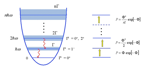
Figure 52: The harmonic oscillator model for the excitation of collective states in nuclei.

The probability that N-phonons will be excited is

$$P_{N} = \sum_{n_{z},\;n_{x}(N=n_{z}+n_{x})}P_{n_{z},n_{x}}=\sum_{n_{z}=0}^{N}P_{n_{z},N-n_{z}}$$ (516)

$$= \sum_{n_{z}=0}^{N}\frac{\left|\chi_{z}(t)\right|^{2n_{z}}\left|\chi_{1}(t)\right|^{2\left(N-n_{z}\right)}}{n_{z}!\left(N-n_{z}\right)!}$$

$$\times \exp\left[-\left|\chi_{z}(t)\right|^{2}-\left|\chi_{x}(t)\right|^{2}\right]$$

$$= \frac{1}{N!}\exp\left[-\left|\chi_{z}(t)\right|^{2}-\left|\chi_{x}(t)\right|^{2}\right]$$

$$\times \sum_{n_{z}=0}^{N}\frac{N!\left|\chi_{z}(t)\right|^{2n_{z}}\left|\chi_{x}(t)\right|^{2\left(N-n_{z}\right)}}{n_{z}!\left(N-n_{z}\right)!}\;.$$

The last sum yields $\left|\phi(t)\right|^{2N}$ , where

$$\left|\phi(t)\right|^{2}\equiv\left|\chi_{z}(t)\right|^{2}+\left|\chi_{x}(t)\right|^{2}.$$ (517)

Thus, one gets the Poisson formula

$$P_{N}=\frac{1}{N!}\;\left|\phi(t)\right|^{2N}\;\exp\left[-\left|\phi(t)\right|^{2}\right].$$ (518)

for dipole excitations of a harmonic oscillator. In Refs. [AW66,AW75] it was shown that the same result can be obtained for quadrupole excitations. Thus, the above result is very general (see Figure 52).

The Poisson equation is very useful. It shows that all one needs to obtain the probability to excite the nth state is to calculate the probability to excite the $N=1$  state with first-order perturbation, $P_{0\rightarrow 1}^{first}=\left|\phi(t)\right|^{2}$  , and use it in the Poisson formula. Although this only holds for a harmonic oscillator system, it has been largely used in many theoretical considerations of more complicated systems. The factor $\exp\left[-\left|\phi(t)\right|^{2}\right]$  accounts for the loss of occupation probability due to the excitation to all states from a given one. It also is responsible for conservation of unitarity, so that $\sum_{N=0}^{\infty}P_{N}=1$ .

XIII.8 Schrödinger equation in a space-time lattice

The operations $\left[{}\right]u_{\alpha}\;$ in the r.h.s. of Eq. (LABEL:(3.12)) is easy. The operation $\left[{}\right]^{-1}u_{\alpha}^{\prime}\;$ is more complicated. The problem is to find the vector $u\;$ in the equation

$$\mathbf{v}=\mathcal{A}^{-1}\;\mathbf{v,\;\;\;\;\;\;\;}\mathrm{where}\mathbf{\;\;\;\;\;v}=\mathcal{A}\;\mathbf{u}$$ (519)

$\mathbf{u}\;$ is a vector composed with the $u^{(j)}=u(r_{j},t)\;$ components of the wave-function $u(r,t)$ . In Eq. LABEL:(3.12) $\mathcal{A}\;$ is a tri-diagonal operator (matrix). In matrix notation

$$\left(\begin{array}[]{c}v_{1}\\ v_{2}\\ .\\ .\\ .\\ ,\\ .\\ v_{N}\end{array}\right){=}\left(\begin{array}[]{ccccccc}A_{1}&0&0&.&.&0&.\\ A_{2}^{-}&A_{2}&A_{2}^{+}&0&.&.&.\\ 0&A_{3}^{-}&A_{3}&A_{3}^{+}&0&.&.\\ .&&&&&&\\ .&&&&&&\\ 0&.&.&.&.&.&A_{\begin{subarray}{c}N\\ \end{subarray}}\end{array}\right)\left(\begin{array}[]{c}u_{1}\\ u_{2}\\ u_{3}\\ .\\ .\\ .\\ u_{N}\end{array}\right).$$ (520)

This involves the following relations

$${A}_{i}^{-}{u}_{i-1}{+A}_{i}{u}_{i}{+A}_{i}^{+}{u}_{i+1}{=v}_{i}.$$ (521)

Assuming a solution of the form

$$u_{i+1}=\alpha_{i}u_{i}+\beta_{i}$$ (522)

and inserting in (521) we find the recursion relations for $\alpha_{i}\;$ and $\beta_{i}:$

$${\alpha}_{i-1}{=\gamma}_{i}{\;A}_{i}^{-}\;,\;\;\;\;\beta_{i-1}=\gamma_{i}\left(A_{i}^{+}\beta_{i}-v_{i}\right)$$ (523)

where

$$\gamma_{i}=-\frac{1}{A_{i}+\alpha_{i}A_{i}^{+}}.$$ (524)

At the end of the lattice we assume $u_{N}=v_{N}\;$ . This implies that $\alpha_{N-1}=0\;$ and $\beta_{N-1}=v_{N}\;$ .

For the problem defined by Eq. (LABEL:(3.12)) we have

$$A_{k}=\frac{1}{i\tau}+2+\frac{\Delta t}{2\hbar\tau}v_{\alpha}^{\left(k\right)},\;\;\;\mathrm{and}\;\;\;\;\;\;\;A_{k}^{-}=A_{k}^{+}=-1.$$ (525)

We can now determine $\alpha_{i}$  and $\beta_{i}$  by running Eqs. (523) backwards from $i=N-2$  down to $i=1$ . Then we use Eq. (522) running forward from $i=2$  to $N$ , assuming that $u_{1}\;$ at the other extreme of the lattice is given by $u_{1}=v_{1}/A_{1}\;$ .

Another way to solve the problem (520) for $u\;$ is by a LU-decomposition, followed by a forward and backward substitution. This method does not need to involve the Dirichlet condition.

Let us assume that the $A$  matrix in (520) can be written as a product of $B\;$ and $U\;$ matrix, where

$${A=LU=}\left(\begin{array}[]{cccccc}b_{1}&c_{1}&0&0&.&.\\ a_{2}&b_{2}&c_{2}&0&.&.\\ 0&a_{3}&b_{3}&c_{3}&.&.\\ .&..&.&..&.&.\end{array}\right)$$ (526)

$$L=\left(\begin{array}[]{cccccc}1&0&0&0&.&.\\ \alpha_{2}&1&0&0&.&.\\ 0&\alpha_{3}&1&0&.&.\\ 0&0&\alpha_{4}&1&.&.\\ .&.&.&.&.&.\\ .&.&.&.&.&.\end{array}\right)\;\;\;U=\left(\begin{array}[]{cccccc}\beta_{1}&\alpha_{1}&0&0&.&.\\ 0&\beta_{2}&\gamma_{2}&0&.&.\\ 0&0&\beta_{3}&\gamma_{3}&.&.\\ .&.&.&.&&\\ .&.&.&.&&\end{array}\right).$$ (527)

Then, $AU=V\;\rightarrow L(Uu)=v$ , or $Ly=V$ .  The elements of  $y$   are

$$\left(\begin{array}[]{c}y_{1}\\ y_{2}\\ .\\ .\\ .\\ y_{N}\end{array}\right)=\left(\begin{array}[]{ccccccc}\beta_{1}&\gamma_{1}&0&0&.&.&.\\ 0&\beta_{2}&\gamma_{2}&0&.&.&.\\ 0&0&\beta_{2}&\gamma_{3}&.&.&.\\ 0&0&.&.&.&.&.\end{array}\right)\;\left(\begin{array}[]{c}u_{1}\\ u_{2}\\ u_{3}\\ .\\ .\\ .\\ u_{N}\end{array}\right).$$ (528)

This can be solved by backwards substitution

$$u_{N}=\frac{y_{N}}{\beta_{N}},\;\;\;\;\;\;\;\;\;\;\beta_{i}u_{i}+\gamma_{i}u_{i+1}=y_{i}\;,$$ (529)

or

$${u}_{i}=\left(y_{i}-\gamma_{1}u_{i}+1\right){\;/\;\beta}_{i}.$$ (530)

The other matrix equation

$$\left(\begin{array}[]{c}\begin{array}[]{cccccc}1&0&0&0&.&.\\ \alpha_{1}&1&0&0&.&.\\ 0&\alpha_{3}&1&0&.&.\\ 0&0&\alpha_{4}&1&0&.\\ .&.&.&.&&.\end{array}\end{array}\right)\;\;\left(\begin{array}[]{c}y_{1}\\ y_{2}\\ .\\ .\\ .\\ y_{N}\end{array}\right)=\begin{array}[]{c}\left(\begin{array}[]{c}v_{1}\\ v_{2}\\ .\\ .\\ .\\ v_{N}\end{array}\right)\end{array}$$ (531)

can be solved by forward substitution

$${y}_{1}{=v}_{1},\;\;\;\;\;\;\;\;\;\;\;\;\alpha_{i}y_{i-1}+y_{i}=v_{i}\;,$$ (532)

or

$${y}_{i}{=v}_{i}{-\alpha}_{i}{y}_{i-1.}$$ ((D.15))

Now, we need to find $\alpha_{i}\;$ and $\beta_{i}\;$ as a function of the original elements of $\mathcal{A}$

$$\left(\begin{array}[]{ccccccc}1&0&0&0&.&.&.\\ \alpha_{2}&1&0&0&.&.&\\ 0&\alpha_{3}&1&0&.&.&\\ .&.&&.&.&&\\ .&.&&.&&.&\\ .&.&&.&&&.\end{array}\right)\left(\begin{array}[]{ccccccc}\beta_{1}&\gamma_{1}&0&0&0&.&.\\ 0&\beta_{2}&\gamma_{2}&0&0&.&.\\ 0&0&\beta_{3}&\gamma_{3}&&.&.\\ .&.&&&.&&\\ .&.&&&&.&\\ .&.&&&&&\beta_{N}\end{array}\right)$$

$$=\left(\begin{array}[]{ccccccc}b_{1}&c_{1}&0&0&0&.&.\\ b_{2}&b_{2}&c_{2}&0&0&.&.\\ 0&a_{3}&b_{3}&c_{3}&0&.&.\\ &.&.&&.&.&\\ &.&.&&.&&.\end{array}\right)$$

which implies

$$b_{1}=\beta_{1},\;\;\;\;b_{2}=\alpha_{2}\gamma_{1}+\beta_{2},\;\;\cdots,\;\;b_{i}=\gamma_{i-1}\alpha_{i}+\beta_{i}.$$

or

$${\beta}_{i}{=b}_{i}{-\gamma}_{i-1}{\alpha}_{i}\;,\;\;\;\;\;\;\;\;\;\;c_{i}=\gamma_{i}.$$ (533)

Also,

$$a_{2}=\beta_{1}\alpha_{2},\;\;\;\;\;a_{3}=\beta_{2}\alpha_{3},\;\;\cdots,\;\;a_{i}=\beta_{i-1}\alpha_{i},$$

or

$$\alpha_{i}=\frac{a_{i}}{\beta_{i-1}}.$$ (534)

Thus, knowing $a_{i,}\;b_{i}$  and $c_{i}$ , one can go upwards with this set of equations to solve the problem.

In our particular case,

$$a_{i}=c_{i}=-1.$$ (535)

Thus, the above equations simplify to

$${\beta}_{1} = {b}_{1},\;\;\;\;\;\;\;\;\;\;\;\;{\beta}_{i}{=b}_{i}{-}\frac{1}{\beta_{i-1}}{\;,\;\;\;\;\;\;\;\;i=2,...,N}$$

$${y}_{1} = {v}_{1},\;\;\;\;\;\;\;\;\;\;\;{y}_{i}{=v}_{i}{+\;}\frac{y_{i-1}}{\beta_{i-1}}{\;\;,\;\;\;\;\;\;\;\;i=2,...,N}$$

$${u}_{N} = \frac{y_{N}}{\beta_{N}},\;\;\;\;\;\;\;\;\;\;\;\;\;{u}_{i}{=\;}\frac{\left(y_{i}+u_{i+1}\right)}{\beta_{i}}{\;\;,\;\;i=N-1,...,1.}$$

XIV Acknowledgments

This work was partially supported by the U.S. DOE grants DE-FG02-08ER41533 and DE-FC02-07ER41457 (UNEDF, SciDAC-2), the the Research Corporation under Award No. 2009-7123, and the JUSTIPEN/DOE grant DEFG02- 06ER41407.

XV References

AAB90

C.E. Aguiar, A.N.F. Aleixo and C.A. Bertulani, Phys. Rev. C 42 (1990) 2180.

AB89

A.N.F. Aleixo and C.A. Bertulani, Nucl. Phys. A 505 (1989) 448.

ABE98

T. Aumann, P.F. Bortignon, H. Emling, Annu. Rev. Nucl. Part. Sci. 48, 351 (1998).

ABS93

T. Aumann, CA. Bertulani and K. Sümmerer., Phys. Rev. C 47 (1993) 1728.

AC79

L.G. Arnold and B.C. Clark, Phys. Lett. B 84, 46 (1979).

AGB82

Y. Alhassid, M. Gai and G.F. Bertsch, Phys. Rev. Lett. 49 (1982) 1482.

Arn73

R.A. Arndt, D.L. Long, L.D. Roper, Nucl. Phys. A 209 (1973) 429.

Aum99

T. Aumann, et al., Phys. Rev. C 59 (1999) 1252.

Aum06

T. Aumann, Europ. Phys. Journ. A 26 (2006) 441.

Ax62

P. Axel, Phys. Rev. 126 (1962) 671.

AW79

A. Winther and K. Alder, Nucl. Phys. A 319 (1979) 518.

Ald56

K. Alder, A. Bohr, T.Huus, B.Mottelson and A.Winther, Rev. Mod. Phys. 28 (1956) 432.

AS64

M. Abramowitz and I.A. Stegun, “Handbook of Mathematical Functions”, (Washington, DC: National Bureau of Standards ), 1964

AW66

K. Alder and A. Winther, “Coulomb Excitation”, (New York: Academic Press), 1966.

AW75

K. Alder and A. Winther, “Electromagnetic Excitation” (Amsterdam: North-Holland), 1975.

Ba62

W.C. Barber, Ann. Rev. Nucl. Sci. 12, 1 (1962).

Bar88

J. Barrette et al., Phys. Lett. B 209 (1988) 182.

BB85

C.A. Bertulani and G. Baur, Nucl. Phys. A 442 (1985) 739.

BB86a

G. F. Bertsch and R. A. Broglia, Physics Today, August 1986, p. 44.

BB86

G. Baur and C.A. Bertulani, Phys. Lett. B 174 (1986) 23.

BB88

C.A. Bertulani and G. Baur, Phys. Rep. 163 (1988) 299.

BB90

F.E. Bertrand and J.R. Beene, Nucl. Phys. A 520 627c (1990).

BB93

G.F. Bertsch and C.A. Bertulani, Nucl. Phys. A 556 (1993) 136.

BB94

C.A. Bertulani and G.F. Bertsch, Phys. Rev. C 49 (1994) 2839.

BBR86

G. Baur, C.A. Bertulani and H. Rebel, Nucl. Phys. A458 (1986) 188.

BC92

C.A. Bertulani and L.F. Canto, Nucl. Phys. A 539 (1992) 163.

BP99

C.A. Bertulani and V. Ponomarev, Phys. Rep. 321, 139 (1999).

BD04

C.A. Bertulani and P. Danielewicz, “Introduction to Nuclear Reactions”, IOP, London, 2004.

Bee90

J. Beene et al., Phys. Rev. C 41, 920 (1990).

Ber04

COULINT: a numerical code for Coulomb excitation at all bombarding energies, C.A. Bertulani, unpublished.

Ber05

C. A. Bertulani, Phys. Rev. Lett. 94, 072701 (2005).

Ber07

C.A. Bertulani, “Nuclear Physics in a Nutshell”, Princeton Press, Princeton, 2007.

BHK09

C.A. Bertulani, Jun-Ting Huang and Plamen Krastev, Mod. Phys. Lett. A 24, 1109 (2009).

BM75

A. Bohr and B. Mottelson, “Nuclear Structure”, vols. I and II, Benjamin, New York, 1975.

BM93

C.A. Bertulani and K.W. McVoy, Phys. Rev. C 48 (1993) 2534.

BP99

C.A. Bertulani and V.Yu. Ponomarev, Phys. Rep. 321 139 (1999).

BR53

L.C. Biederharn and M.E. Rose, Rev. Mod. Phys. 25, 729 (1953).

BS92

C.A. Bertulani and A. Sustich, Phys. Rev. C46 (1992) 2340.

BS94

D. Brink and G.R. Satchler, “Angular Momentum”, Oxford University Press, Oxford, 1953.

Ca96

C.A. Bertulani, L.F. Canto, M.S. Hussein and A.F.R. de Toledo Piza, Phys. Rev. C 53 (1996) 334.

Cob97

A. Cobis, D. Fedorov, A. Jensen, Phys. Rev. Lett. 79, (1997) 2411 .

Dan98

B.V. Danilin, I.J. Thompson, J.S. Vaagen, M.V. Zhukov, Nucl. Phys. A 632 (1998) 383.

DB88

S. S. Dietrich and B. L. Berman, At. Data and Nucl. Data Tables, 38 (1988) 199.

EB92

H. Esbensen and G. F. Bertsch, Nucl. Phys. A 542, 310 (1992).

EBB95

H. Esbensen, G.F. Bertsch and C.A. Bertulani, Nucl. Phys. A 581 (1995) 107.

EB05

H. Esbensen and C.A. Bertulani, Phys. Rev. C 65, 024605 (2002).

Ed60

A.R. Edmonds, “Angular Momentum in Quantum Mechanics”, Princeton University Press, Princeton, New Jersey, 1960.

Efr96

V. Efros, W. Balogh, H. Herndl, R. Honger, H. Oberhummer, Z. Phys. A 355 (1996) 101.

EG88

J.M. Eisenberg and W. Greiner, “Excitation Mechanisms of the Nucleus”, (North-Holland, Amsterdam, 1988).

Fe24

E. Fermi, Z. Physik, 29, 315 (1924).

Fe25

E. Fermi, Nuovo Cimento 2 (1925) 143.

Few84

M.P. Fewell, Nucl. Phys. A 425 (1984) 373.

FS65

H. Frauenfelder and R.M. Steffen, “Alpha-, beta- and gamma-ray spectroscopy”, Vol. 2, ed. K. Siegbahn.

Gla01

T. Glasmacher, Nucl. Phys. A 693, 90 (2001).

Go02

H. Goldstein, C.P. Poole, C.P. Poole Jr. and J.L. Safko, “Classical Mechanics” (Prentice Hall, 3rd edition), 2002.

GR80

I.S. Gradshteyn and I.M. Ryzhik, “Table of Integrals, Series, and Products” (New York: Academic Press ), 1980.

GT48

M. Goldhaber and E. Teller, Phys. Rev. 74, 1046 (1948).

GZK66

K . Greisen, Phys. Rev. Lett. 16 (1966) 748; G .T. Zatsepin and V. A. Kuzmin, Zh. Eksp. Teor. Fiz. 4 (1966) 114, JETP Lett. 4 (1966) 78.

Haik05

H. Simon, Technical Proposal for the Design, Construction, Commissioning, and Operation of the ELISe setup, GSI Internal Report, Dec. 2005.

Iek93

K. Ieki et al., Phys. Rev. Lett. 70 (1993) 730.

Ja75

J.D. Jackson, “Classical Electrodynamics” (New York: Wiley), 1975.

Kam87

M. Kamimura et al., Prog. Theor. Phys. Suppl. 89, 1 (1986); N. Austern et al., Phys. Rep. 154, 125 (1987).

Le74

A. Leprêtre et al., Nucl. Phys. A 219 (1974) 39.

LL89

L.D. Landau and E.M. Lifshitz, The classical theory of fields, 4th ed. (Pergamon, Oxford, 1979).

Ma75

N. Marty, M. Morlet, A. Willis, V. Comparat and R. Frascaria, Nucl. Phys. A 238 (1975) 93.

Mer74

S.P. Merkuriev, Sov. J. Nucl. Phys. 19 (1974) 222.

Mo88

S. Mordechai et al., Phys. Rev. Lett. 61 (1988) 531.

Mot94

T. Motobayashi et al., Phys. Rev. Lett. 73 (1994) 2680.

Mye77

W.D. Myers, W.G. Swiatecki, T. Kodama, L.J. El-Jaick and E.R. Hilf, Phys. Rev. C 15, 2032 (1977).

Nak06

T. Nakamura et al., Phys. Rev. Lett. 96, 252502 (2006).

Oga03

K. Ogata, M. Yahiro, Y. Iseri, T. Matsumoto and M. Kamimura, Phys. Rev. C 68, 064609 (2003).

Oga06

K. Ogata, S. Hashimoto, Y. Iseri, M. Kamimura and M. Yahiro, Phys. Rev. C 73, 024605 (2006).

OB09

K. Ogata and C.A. Bertulani, Prog. Theor. Phys. (Letter) 121 (2009) 1399.

OB09b

K. Ogata and C.A. Bertulani, in preparation.

Pry48

M. H. L. Pryce, Proc. Roy. Soc. A195, 62 (1948).

Pus96

A Pushkin, B Jonson and M V Zhukov, J. Phys. G 22 (1996) L95.

PW71

R. Pitthan and Th. Walcher, Phys. Lett. 36 B (1971) 563.

Rit93

J. Ritman et al., Phys. Rev. Lett. 70 (1993) 533.

Sa51

R.G. Sachs and N. Austern, Phys. Rev. 81, 705 (1951).

Sch54

L.I. Schiff, Phys. Rev. 96, 765 (1954).

Sch93

R. Schmidt et al., Phys. Rev. Lett. 70 (1993) 1767.

She54

R. Sherr, C.W. Li and R.F. Christy, Phys. Rev. 96 (1954) 1258.

Shi95

S. Shimoura et al., Phys. Lett. B 348 (1995) 29.

Sie37

A.J.F. Siegert, Phys. Rev. 52, 787 (1937).

SIS90

Y. Suzuki, K. Ikeda, and H. Sato, Prog. Theor. Phys. 83, 180 (1990).

SJ50

H. Steinwedel and H. Jensen, Z. Naturforschung 5A, 413 (1950).

Sud01

T. Suda, K. Maruayama, “Proposal for the RIKEN beam factory”, RIKEN, 2001; M. Wakasugia, T. Suda, Y. Yano, Nucl. Inst. Meth. Phys. A 532, 216 (2004).

Tem55

G.M. Temmer and N.P. Heydenburg, Phys. Rev. 98, 1198 (1955).

Thoe99

M. Thoennessen et al., Phys. Rev. C 59, 111 (1999).

Ti04

D. R. Tilley et al., Nucl. Phys. A 745, 155 (2004).

Ve70

A. Veyssière, H. Beil, R. Bergère, P. Carlos and A. Leprêtre, Nucl. Phys. A 159 561 (1970).

VGB90

A.C. Vasconcellos-Gomes and C.A. Bertulani, Nucl. Phys. A 517, 639 (1990).

WB65

A. Winther and J. De Boer, “A Computer Program for Multiple Coulomb Excitation”, Caltech, Technical report, November 18, 1965. Reprinted in [AW75].

WW34

C.F. Weizsacker, Z. Physik, 612 (1934); E.J. Williams, Phys. Rev. 45, 729 (1934).

Zhu93

M.V. Zhukov, B.V. Danilin, D.V. Fedorov, J.M. Bang, I.J. Thompson and J.S. Vaagen, Phys. Rep. 231, 151 (1993).