Radial Distribution of X-ray Point Sources near the Galactic Center
Abstract
We present the log-log and spatial distributions of X-ray point sources in seven Galactic Bulge (GB) fields within 4∘ from the Galactic Center (GC). We compare the properties of 1159 X-ray point sources discovered in our deep (100 ks) Chandra observations of three low extinction Window fields near the GC with the X-ray sources in the other GB fields centered around Sgr B2, Sgr C, the Arches Cluster and Sgr A* using Chandra archival data. To reduce the systematic errors induced by the uncertain X-ray spectra of the sources coupled with field-and-distance dependent extinction, we classify the X-ray sources using quantile analysis and estimate their fluxes accordingly. The result indicates the GB X-ray population is highly concentrated at the center, more heavily than the stellar distribution models. It extends out to more than 1.4∘ from the GC, and the projected density follows an empirical radial relation inversely proportional to the offset from the GC. We also compare the total X-ray and infrared surface brightness using the Chandra and Spitzer observations of the regions. The radial distribution of the total infrared surface brightness from the 3.6 band m images appears to resemble the radial distribution of the X-ray point sources better than predicted by the stellar distribution models. Assuming a simple power law model for the X-ray spectra, the closer to the GC the intrinsically harder the X-ray spectra appear, but adding an iron emission line at 6.7 keV in the model allows the spectra of the GB X-ray sources to be largely consistent across the region. This implies that the majority of these GB X-ray sources can be of the same or similar type. Their X-ray luminosity and spectral properties support the idea that the most likely candidate is magnetic cataclysmic variables (CVs), primarily intermediate polars (IPs). Their observed number density is also consistent with the majority being IPs, provided the relative CV to star density in the GB is not smaller than the value in the local solar neighborhood.
Subject headings:
Galaxy: bulge — X-ray: binaries — X-ray: population1. Introduction
The Chandra X-ray Observatory has opened a new era in studies of the X-ray source population in the Galactic Bulge (GB). A series of shallow and deep Chandra observations in the Galactic Center (GC) region have revealed 1000 X-ray point sources in a 2∘ 0.8∘ region (Wang et al., 2002) and 2357 X-ray point sources in a region around the Sgr A* (Muno et al., 2003, hereafter M03). An additional 2000 sources found in the Bulge Latitude Survey (BLS, two 0.8∘ 1.5∘ regions) provide the initial results for the latitude distribution of the GB sources (Grindlay et al., 2009). The X-ray luminosities and relatively hard spectra ruled out that the majority of the GC X-ray point sources are normal stars, active binaries, young stellar objects, or quiescent low mass X-ray binaries (qLMXBs) (M03). From the lack of real matches between the bright infrared (IR, ) and X-ray sources in the Sgr A* field, Laycock et al. (2005, hereafter L05) concluded that high mass X-ray binaries (HMXBs) cannot account for more than 10% of the X-ray sources in this region. While the leading candidate that fits the properties of these X-ray sources is now magnetic cataclysmic variables (CVs) (Muno et al., 2004, L05), the relatively hard X-ray spectra of some of the most recently discovered qLMXBs imply qLMXBs could be misrecognized as CVs and be more common in the GB than thought in the past (Wijnands et al., 2005; Bogdanov et al., 2005). Infrared (IR) searches for the counterparts of these GB X-ray sources have been actively pursued (e.g. Muno et al. (2005)), but the exact nature of the majority of the sources is still elusive due to high obscuration by dust and source confusion by the high star density.
We have conducted a series of deep (100 ks) Chandra observations of three low extinction Window fields – Baade’s Window (BW), Stanek’s Window (SW; Stanek 1998) and the ”Limiting Window” (LW) – near the GC (§2). These Window fields allow us to observe the GB X-ray population and their Galactic radial distribution with minimal obscuration by dust. We have discovered 1159 X-ray point sources in these fields. We compare their distributions with X-ray sources in other GB fields – the Sgr B2, Sgr C, Arches Cluster and Sgr A* fields. We present a new approach using quantile analysis (§3) to minimize the systematic errors in flux estimation, to classify sources by their X-ray spectral types and investigate their radial distribution. We compare the X-ray distribution with the known models of the stellar distribution (§4) and investigate the nature of the X-ray population (§5). See also van den Berg et al. (2009), where we put constraints on the nature of the X-ray source populations from the optical point of view, using HST observations of the Window fields taken simultaneously with the Chandra exposures. This work is part of our Chandra Multi-wavelength Plane (ChaMPlane) Survey designed to measure the space density and probable nature of the low-luminosity accretion-powered sources in the Galaxy (Grindlay et al., 2005).
2. Observations and Data Analysis
We performed Chandra/ACIS-I observations of BW on 2003 July 9 (Obs. ID 3780), SW on 2004 February 14/15 (Obs. ID 4547 and 5303), and LW on 2005 August 19/22 and October 25 (Obs. ID 5934, 6362 and 6365). Due to technical constraints, the SW and LW observations were segmented into a few pointings, which we stacked for further analysis. Table 1 summarizes the observational parameters and X-ray source statistics of the Window and other GB fields analyzed in this paper. For the Sgr A* field, we use the results from a 100 ks observation (Obs. ID 3665) for easy comparison with other GB fields that were observed with similar exposure times, and we have also stacked 14 observations from the archive, totaling 750 ks exposure.
We have analyzed the data as a part of the ChaMPlane survey. For uniform analysis of all the ChaMPlane fields, we have developed a series of X-ray processing tools, mainly based on version 3.4 of the CIAO package (Hong et al., 2005, hereafter H05)222Some of the fields were processed by the tools based on version 3.1 of the CIAO package, but the difference between two versions is minimal.. After initial screening of the CXC level-2 data (e.g. select the events in good time intervals during which the background fluctuates above the mean level), we detect X-ray point sources with a wavelet algorithm (wavdetect, Freeman et al. 2002) with a significance threshold of . The wavdetect routine is run on each individual observation and the stacked data set if available. Multiple observations are considered stackable (the SW, LW and Sgr A* fields here) if the aimpoints are on the same detector (ACIS-I or ACIS-S) and they are within 1 of each other.
In H05, we used source detections in the broad (: 0.3–8.0 keV) band. We now also incorporate source detections in the soft (: 0.3–2.5 keV) and hard (: 2.5–8.0 keV) bands in addition to the broad band. We establish a unique source list by cross matching the three detection lists based on the relative distance of possibly identical source pairs (the closest pairs) in the three different bands. The relative distance () of two sources is defined by the ratio of the source distance to the quadratic sum of the positional errors. Note that there is no astrometric offset among the images in the three bands. The positional errors of sources are calculated by an empirical formula based on the MARX333http://space.mit.edu/CXC/MARX/. simulations (Eq. 5 in H05).
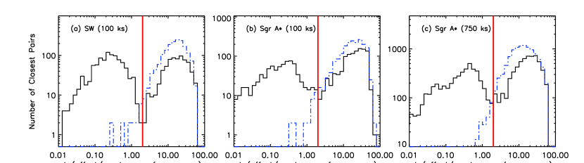
Establishing a unique source list is straightforward in relatively un-crowded fields such as the Window fields, but it can be tricky in heavily populated fields and in very deep exposures such as the stacked Sgr A* dataset. Fig. 1 shows the distributions of the relative separations of nearest-neighbor source pairs among the three detection bands, , , and . As examples, we compare the 100 ks observations of the Stanek Window and Sgr A* field, and the 750 ks stacked dataset of the Sgr A* field. A source detection in each band contributes two pairs to the distribution, one from each of the other two bands.
The bimodal shape of the distribution indicates two types of the pairs contribute to the distribution: one type consists of the truly identical sources detected in different bands and the other consists of random pairs of unrelated sources. The distribution of the random pairs can be estimated by introducing an arbitrary astrometric offset in the source position between the detection bands. The (blue) dashed-dotted line in Fig 1 shows such an example (1 offset in both R.A. and Dec.), the shape of which closely resembles the right side of the bimodal distribution of original sources. The slight excess over the original distribution is due to the real pairs being transformed into new random pairs by the positional offset.
After visual inspection of the raw images and the distributions of the relative distances in Fig. 1, we use a simple cut (2.0, red vertical line) for establishing the unique source list. The cut is sufficient for identifying virtually 100% of the unique sources detected in multiple bands. From the distributions of the relative distances of the random pairs, we estimate that the false random matches surviving the cut ranges from 10 to 25 for the 100 ks observations. The corresponding number of independent sources that might have lost by the false random matches ranges from 5 to 10 ( 1%) for the 100 ks observations and about 100 for the stacked Sgr A* field ( 3%).
When multiple detections in the three bands are identified as a unique source, we select the one with the smallest positional error for the unique source list. We note that the final source position and error could be derived from a form of weighted average of astrometric properties of multiple detections. However, the and band detections are not entirely independent from the band detection. Therefore, in order to avoid unnecessary complication in the analysis, we simply take the astrometric (and photometric) properties of the source with the smallest positional errors, which is the detection with the highest significance among the three bands.
As a sanity check, we compare our detection with the available catalogues in the literature. M03 provided a catalogue of the 2357 X-ray point sources discovered in the 690 ks exposure (626 ks of GTIs) of the Sgr A* field, Muno et al. (2006, hereafter M06) for the 397 point sources in the 100 ks exposure of the Sgr B2 field (Obs. ID 944) and Wang et al. (2006, hereafter W06) for the 244 X-ray point sources in the 100 ks exposure of the Arches Cluster (Obs. ID 4500). The majority (%) of these sources are also detected in our analysis or vice versa if our source list is shorter than theirs. A small fraction of the sources are missing due to many subtle differences in the detection methods and the selection criteria for the lists such as the detection energy bands (0.5–8, 0.5–1.5 and 4–8 keV in M03 or 1–4, 4–9 and 1–9 keV in W06), the pointing or GTI selections (e.g. Obs. ID 1561 was not included in our analysis in the stacked Sgr A* field). In addition, in the case of W06, their high significance threshold (10-7 except for the inner region, about 10 counts in their broad band, 1–9 keV) is one of the main reasons for the difference (244 vs. 423) in the total number of the source detections. M03 and M06 list all the source detections including ones with negative counts in their broad band (0.5–8 keV). Our source list includes the detections with net counts 1 in the band (0.3–8 keV).
After source detection, we perform aperture photometry on each source to extract the basic source properties such as net count and net count rate in the conventional energy bands (: 0.5–2.0, : 2.0–8.0 and : 0.5–8.0 keV) and energy quantiles in the broad band (: 0.3–8.0 keV). For the sources that fall near other sources, we carefully revise the aperture of the source regions by excluding overlapping sections to minimize the contamination from the neighbors (H05). Table 2 lists a part of the source catalog with selected source properties used in this paper. The complete list for the Window and other GB fields is available in the electronic edition.
3. Flux estimation by Quantile classification
In order to compare source distribution in various regions of the sky with diverse extinctions, it is necessary to correct for the interstellar absorption and use the unabsorbed source flux of individual sources. However, such a calculation is not trivial for X-ray sources with diverse spectral types as found in Galactic plane fields since faint sources are unsuitable for spectral fitting. Moreover, the relatively large extinction in the GB fields and its usually-unknown field-and-distance dependent variation make it difficult to identify the underlying X-ray spectral model (e.g. power law vs. thermal Bremsstrahlung, etc). An inaccurate assumption of the spectral model when estimating flux introduces systematic errors that often exceed the statistical errors. We therefore employ quantile analysis (Hong et al., 2004, hereafter H04), which is relatively free of the count-dependent bias inherent in X-ray hardness ratio or X-ray color analysis, and so provides a better measure for classifying X-ray sources in the GB fields. In the following, the energy quantile corresponds to the energy below which of the counts are detected. e.g. is the median energy.
3.1. Quantile Analysis
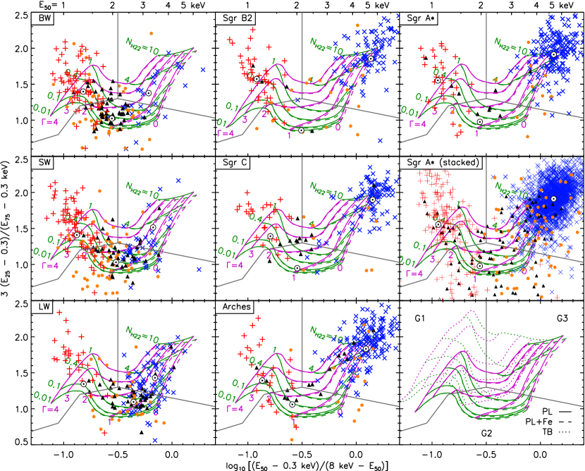
Fig. 2 shows the quantile diagrams of the X-ray sources ( in ) in the selected GB fields overlaid with grids for a simple power law model (PL, solid lines) and a power law plus an iron emission line (PL+Fe, dashed) at 6.7 keV with 0.4 keV equivalent width (EW, see §3.2 for the motivation of the line choice). The lower right panel also includes a grid for the thermal Bremsstrahlung model (TB, dotted). The here is calculated based on the statistical errors () using small-number statistics from Gehrels et al. (1986) (see also Kim et al. (2004)). The difference in the model grids between PL and PL+Fe is only evident in the highly absorbed or spectrally very hard section of the diagram (the right side) because a small iron line ( 6 keV with 1 keV EW) does not make a noticeable difference in three quantiles of the soft sources.
Relatively insensitive to the extinction, the sources around are present in every field and they appear unabsorbed and intrinsically soft regardless of the assumed model class (PL, PL+Fe or TB). Foreground thermal sources such as coronally active stars fit the description. The location of relatively hard sources in the diagram varies with the field extinction. In the Window fields, the hard sources are relatively unabsorbed, but on approach to the GC, there is an increasing trend in the source number with both the average absorption and the intrinsic hardness, when compared to a simple power law model. For instance, in BW most sources have power law photon index ( and , whereas in LW many sources lie in and . In the Sgr A* field and the rest, most of the hard sources are heavily absorbed with and on average, well separately from the foreground sources. We explore this more in Section 3.2.
The quantile diagrams nicely illustrate the spectral diversity of the X-ray sources in the GB fields, but poor photon statistics also contributes to the scatter. To reduce systematic errors caused by poor statistics in assigning spectral types while allowing the spectral diversity of the sources in each field, we divide the diagram into three groups as shown by the (grey) lines originating at (0.5, 1.3). The left section represents most foreground thermal sources (: soft group), the middle section most unabsorbed accreting sources (: medium group), and the right section the absorbed thermal or accreting sources (: hard and absorbed group). The division between and is devised to be somewhat robust444Under the PL model, the boundary of the and groups stays in roughly between =2 and 3. against variations in detector response between ACIS-I and ACIS-S (see H04; H05); or induced by gradual loss of low energy response. The final results (e.g. log-log distributions) are not sensitive to small changes of the group boundaries (e.g. shifting the boundaries by 0.1 in or ). The mean quantiles for each group (marked by ) are calculated by the stacked photons of the sources in the group with and net counts (to avoid being dominated by a few bright sources) in . For a given model class (e.g. PL), we estimate the spectral model parameters (e.g. and ) of the sources in each group using the mean quantiles.
3.2. Spectral hardening vs. radial offset from GC
Table 3 summarizes the group mean quantiles of the and sources and corresponding model parameters under the PL and PL+Fe models. The sources in the high extinction fields are omitted in the Table since they are mostly foreground sources. For comparison, the table also shows the model parameters estimated from spectral model fits. In order to increase photon statistics, we stacked the spectra of sources within a group with net counts for spectral fitting555One can use a spectral model fit on individual sources with net counts 200–300, but in order to establish more reliable statistics for the presence of the line emission for the group, we also stack moderately bright sources with net counts up to 1000. and the spectra were binned to have at least 40 counts in each bin. The model used is a power law plus an iron emission line for which we have chosen the 6.7 keV Fe XXV He- line because it has also been observed in the spectra of the X-ray point sources in the deep survey of the Sgr A* field (M03), the shallow survey of the GC strip (Wang et al., 2002), and other parts of the Galactic plane (Ebisawa et al., 2005). The 6.4 keV neutral iron line is also present in some sources of the GB fields, but it is generally more prominent as unresolved diffuse emission (Wang et al., 2002). Note our aperture photometry is designed to minimize possible contamination of the diffuse emission through background subtraction (H05). We have chosen the 0.4 keV EW for the line in quantile analysis (and the log-log distribution later) because it lies in the EW range estimated by spectral model fits on the sources and Muno et al. (2004) found a similar value ( 0.4 keV) for the bright sources in the Sgr A* field.
Under the PL model, both groups show a trend of increasing hardness of the intrinsic spectra on approach to GC (i.e. for the Window fields vs. for other GB fields). This apparent trend can be attributed to a few factors.
In the case of the sources in the Window fields, the group contains a large number of foreground coronal sources and background AGN in addition to the GB sources. For instance, in the BW and SW, about 70% of the sources with in the band are background AGN (see Fig. 5 in §4). Therefore, the group is perhaps too contaminated for the apparent trend to be taken for real.
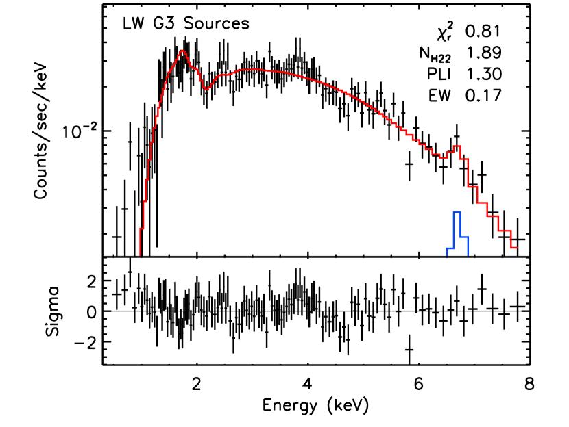
The similar trend in the group appears to be more realistic. However, comparing the PL+Fe model grid with the PL model grid in the quantile diagram suggests this trend can be an artifact of using the PL model at least in part. Indeed the trend is alleviated under the PL+Fe model as shown by the model parameters estimated by both quantile analysis and the spectral fits (Table 3). Poor statistics in the sources of BW and SW does not allow any meaningful constraint of the iron line emission in the spectra, but the stacked spectrum of the sources in the LW does show a clear hint of the 6.7 keV line (Fig. 3, see also Revnivtsev et al (2009)). The relatively weak line feature (EW 0.17 keV) in the LW can be explained by the relatively large contribution of AGN in the group compared to other GB fields (see Fig. 5 in §4).
With the inclusion of a 6.7 keV line, the power law index () becomes largely consistent across the GB fields with the possible exception of the Sgr B2 or C field (see §5.4). The result indicates that the galactic X-ray sources in the LW field may be the same type of sources as seen in the other GB fields closer to the GC. If true, the GB X-ray sources indeed extend out to at least 1.4∘ from the GC.
3.3. Flux Estimates
Based on the group model parameters, we estimate the source flux in the conventional energy bands, using the instrument response files at the aim point and scaling them for source position on the detector by the exposure map (H05)666The latest CIAO tools (ver 3.4 or higher) can calculate the response files appropriate for each source location.. For the stacked data, we use the average response files weighted by the exposure of each observation.
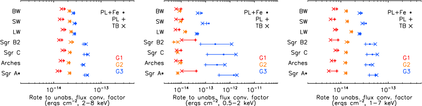
The quantile diagram can assign the model parameters (e.g. =1.7 vs. 1.0) appropriate to a given model class for the sources, but it cannot determine which model class (e.g. PL vs. TB) is right for the sources. A certain model can only be ruled out when the derived values of the parameters are unphysical or with external information (e.g. optical identifications). In order to estimate the systematic errors arising from the improper choice of the model class, we compare flux estimates under three different model classes: PL, PL+Fe and TB. In order to see the significance of the difference among these models, Fig. 4 compares the conversion factor of count rate to unabsorbed flux for sources near the aim point in each group under the three model classes. In the case of the band, the difference between the model classes is very small, but in the band, the conversion factor can differ by more than a factor of 10. We take the largest difference in the flux estimates among the three model classes as the systematic errors () and compare them with the pure count-based statistical errors (). For the flux estimates in the band, and we get for 87% of the sources with , and for 62% even with . In the band, can be larger than 1000%, and we get only for 28% with and for 16% with .
This exercise does not explore all the possible model classes, but the results indicate the band flux estimates in this method are robust and relatively insensitive to the choice of the model classes. However, the band flux estimates can be dominated by the systematic errors arising from improper selection of the spectral model. The fundamental difference between the and band is that the band is very sensitive to the range of interstellar absorption in the GB fields, cm-2, while the band is not. In the following, we limit our discussion to the band results using the sources with in (‘x’s and triangles in Fig. 2), which are likely to be GB sources (and AGN) rather than the foreground sources. See also van den Berg et al. (2009) for the spectral choices for the flux estimates in . If the number of counts in the stacked spectrum of a quantile group (, or ) were large enough, a spectral fit would be better suited for determining the underlying spectral model and its parameters, but a fit can also leave ambiguity over the correct spectral model. Since in the band the difference driven by the model class is less significant than the statistical errors, we simply use the model parameters estimated by quantile analysis.
4. source distribution
4.1. Eddington and Malmquist Biases
In order to explore the effect of the Eddington bias (EB), which makes the faintest sources appear brighter than they really are, we simulate three spectral types of sources (one for each group) based on the group mean quantiles for each field. Using the MARX simulation code, we generate the sources with net counts () from 5 to 400, using a distribution to cover the wide count range efficiently. We scatter 200 – 250 of these sources randomly over the real events and apply the regular analysis procedure. We repeat the procedure 1000 times. The fake sources are not allowed to overlap each other but they can fall on top of the real sources. The results indicate that the EB is noticeable in the sources with 10 counts, which can appear as bright as 15 – 20 count sources, depending on the field (or up to 30 count sources for the stacked Sgr A* field). Since we consider sources with in the band, which corresponds to 16 – 20 counts at least ( 30 counts for the stacked Sgr A* field), we expect EB is not a major contributor to the errors of the following distributions.
The Malmquist bias (MB) is due to the exposure dependent volume (depth) coverage. The MB is usually a concern for luminosity distributions but not for log-log distributions in the apparent (detected) flux space. However, the log-log distributions in the unabsorbed flux space can be subject to the MB when strong interstellar absorption limits the depth of the view, underestimating the true distribution. Therefore, the faint end of the log-log distribution can be lower than the true distribution and so the MB counteracts the EB to some extent.
With 100 ks exposure, all the sources with an unabsorbed flux ergs cm-2 s-1 can be detected at the far side of the Galaxy with in under the assumption of the total integrated absorption777 Assuming the absorption to the GC to be 6 cm-2 (Baganoff et al., 2003) and the symmetry with respect to the GC. of . Therefore the MB is not a concern for sources with ergs cm-2 s-1 (or ergs cm-2 s-1 for the Window fields) under the assumption of a power law wth =1.0 for the X-ray spectrum. This does not mean we can access X-ray sources of a certain luminosity uniformly all the way through the Galaxy. For instance, the unabsorbed flux of ergs cm-2 s-1 corresponds to ergs s-1 at the GC (8 kpc, ) and ergs s-1 at 20 kpc ( ). The situation is a bit more tricky since under the quantile group method we assign fixed spectral parameters with a fixed value for the X-ray spectra of all the sources in each group, which in fact have a diverse distribution (e.g. the group in the Sgr A* field). However, the sources with an unabsorbed flux of ergs cm-2 s-1 in this method are free of the MB for 100 ks exposure. The MB can be a problem for the and sources in the high extinction fields, but their contribution in the log-log distribution of the band is negligible compared to the sources.
4.2. Sky Coverage
For the log-log distribution, we need to know the sky coverage as a function of flux. In order to minimize the systematic errors associated with spectral type assignment, we calculate the sky coverage of each source based on the detected photon counts in the three energy bands as follows (Cappelluti et al. 2005; H05). For each observation, we generate the background-only images by removing the counts in the source regions in the image and filling the region with the counts using the statistics in the surrounding regions (dmfilth)888http://cxc.harvard.edu/ciao/ahelp/dmfilth.html. At every pixel in the background images, we calculate the minimum source counts required for detection with . For the sky coverage of a given source, we take the sky area where the minimum counts are less than the net counts of the source in the band. These sky coverage values agree well with those expected from the simulated sources of three spectral types using the MARX (§4.1). On average, they are within 10% for the cases with , which indicates this method accounts for the completeness as well.
4.3. The log-log and Radial Distributions
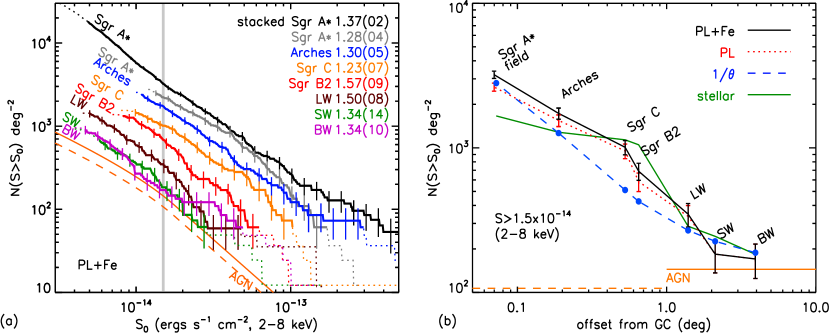
The log-log and radial distributions of the X-ray sources in the GB fields are shown in Fig. 5a & b respectively. The log-log distribution was computed using sources with in the band, under both the PL and PL+Fe models described in §3, with the latter result plotted in Fig. 5a. The source number-density values plotted against angular distance from Sgr A* in Fig. 5b are projected from the log-log distributions at the flux value indicated by the vertical grey line ( ergs cm-2 s-1) in Fig. 5a. As seen in Fig. 5b, the total source densities under the PL model are slightly lower than the same under the PL+Fe model in the high extinction fields, while both distributions under these models are nearly identical in the three low extinction Window fields.
For clarity, we define the statistically robust section of each distribution in Fig. 5a and emphasize it with a solid line. This ”solid section” is defined to contain contributions from at least 10 or more sources, which set the upper limit of the range (e.g. ergs cm-2 s-1 for Sgr C). The lower limit is set by the flux value at which the sky coverage of the contributing sources is greater than 50% of the maximum sky coverage i.e. the full field of view (FoV) (e.g. ergs cm-2 s-1 for Sgr C). In this way, we avoid the statistical bias or fluctuation due to either low source statistics at the bright end of the accessible flux range or limited sky coverage at the faint end of the range. The portion of each distribution not meeting the above criteria is dotted.
The slope () of the log-log distribution is calculated by a power law fit () to the solid line section of the distribution. The -axis error of the distribution is given by the quadratic sum of the statistical error (shown in the figure) and a constant systematic error (, the difference between the PL and PL+Fe model). As expected for the narrow FoV of ACIS-I observations, the slopes of the log-log distributions are largely consistent with the -1.5 slope within except for the stacked Sgr A* field, which shows a hint of the actual deviation () from the -1.5 slope. Note the calculated slopes are only for guiding purpose, and they should not be taken seriously for representing the population since a simple power law does not fit some of the distributions very well.
The AGN distribution is taken from Kim et al. (2007), using a power law model with = 1.7 for the X-ray spectra. The (orange) dashed line indicates the reduced AGN population that can be seen through the high extinction fields such as the Sgr A* field, since the unabsorbed flux is corrected for the average absorption of the X-ray sources, mostly Galactic and centered around the GC, which should be about half of the total absorption for the AGN. For simplicity, we correct another for the AGN seen in the high extinction fields.
For the Sgr A* field, we plot the results from both the stacked data (black) and the 100 ks exposure (grey) in Fig. 5a and use only the stacked data in Fig. 5b. The spectral models from the 100 ks exposure are used for both data sets for fair comparison with other fields and to avoid any spectral parameter driven variations between two exposures for the Sgr A* field. The distribution of the stacked data is higher at ergs cm-2 s-1 than the same for the 100 ks exposure. A few factors such as the MB999Note that the unstacked Sgr A* field (Obs. ID 3665) has the shortest GTI (88 ks) among the seven fields. are responsible for the difference, but the main cause of the difference is suspected to be the X-ray variability of the sources. The stacked data (750 ks) simply have a better chance of detecting the sources or catching high flux states of the sources than for the shorter exposure (100 ks). For instance, the 20 brightest sources in the band in the 100 ks observation of the Sgr A* field are found to be about 30% brighter on average in the stacked data set, and five of the 20 brightest sources in the stacked data were not detected in the 100 ks observation. This variation qualitatively agrees with the change seen in the log-log distributions, but the diverse nature of the X-ray variability and duty cycles makes it hard to quantify the resulting difference in the log-log distributions.
The radial distribution is generated from the sources with ergs cm-2 s-1, plotted over the stellar distribution (green) and the distribution (blue dashed). Both the stellar and distributions are averaged over the ACIS-I FoV () of the GB fields. The value for the radial distribution is chosen as a compromise between having sufficient source statistics in the Window fields ( ergs cm-2 s-1) and avoiding statistical biases in the high extinction fields ( ergs cm-2 s-1). The curve resulting under the PL+Fe model (black solid) is more centrally concentrated around the GC than the PL model (red dotted).
The stellar distribution is derived from the Galactic stellar models compiled by M06, and it consists of a central spherical cluster (, Eq. 1 in M06), a central disk (, Eq. 2 in M06), a triaxial ellipsoidal GB (, Eq. 3 in M06) and a Galactic disk (, Eq. 6 in M06; for the origin of the formulae, see also Launhardt et al. 2002, hereafter L02; Kent et al. 1991, hereafter K91). For the first three components (, & ), we use the formula and the parameter values in L02 and M06. For the Galactic disk component (), M06 use a simple exponential form in K91 and employ 1011 for the total Galactic disk mass for the overall normalization, but since the first three components are mainly for the stellar mass, we believe this is an overestimate. Therefore, we use a normalization that matches the local stellar mass density of 0.044 pc-3 (Robin et al., 2003). This gives for the whole disk, which is roughly consistent with the estimate by Robin et al. (2003) ( )101010The small difference is mainly due to the difference in the assumption of the distance to the GC: 8 kpc for the model used here, and 8.5 kpc for Robin et al. (2003).. Since we expect both the X-ray and stellar sources are centrally concentrated around the GC, in Fig. 5b we further assume that all detected hard Galactic X-ray sources are at a distance of 6 – 10 kpc, which is justified given that the stellar models predict that of sources along the line of the sight of the GB fields lie in the same distance range. Note the central concentration also makes our normalization change of the Galactic disk component less important in the outcome, but we find that the change makes this Galactic stellar mass model consistent with other Galactic stellar number density models (see §5.1 and Table 4). These stellar model components have about a factor of two uncertainty (M06, L02).
The normalization of the stellar and distributions is set by a simple fit to the radial-distribution curve under the PL+Fe model (Fig. 5b). We use the stacked result for the Sgr A* field. The radial distribution shows the GB X-ray sources are highly concentrated at the GC, more than the stellar distribution. It also shows the hard GB X-ray sources extend out to 1.4∘ from the GC, roughly following an empirical relation of with some excess in the Arches Cluster, Sgr C and Sgr B2 fields.
The excess of the X-ray source to stellar distribution near the GC does not appear as prominent if we use the 100 ks exposure of the Sgr A* field at ergs cm-2 s-1. However, the trend of the relative excess of the X-ray sources toward the GC is present from the Sgr B2 to Sgr A* field (e.g. the Sgr B2 field has a deficit under the current relative normalization in Fig. 5b), and the log-log distributions of the 100 ks exposure and the stacked Sgr A* field become more consistent at ergs cm-2 s-1. Therefore, the excess of X-ray sources toward the GC with respect to the considered stellar model appears real. We explore this excess in more detail in Section 5.1.
5. Discussion
We find that the number-density of the hard X-ray sources in the GB is significantly elevated above the AGN density out to at least the LW at 1.4∘ separation from Sgr A* (Fig. 5a). Furthermore, although empirical (see Fig. 6 for the composition of the stellar population), the radial distribution of the hard X-ray sources roughly follows a relation out to this field (Fig. 5b). This discovery suggests that all such sources observed within at least 200 pc of the GC belong to the same centrally concentrated population. The similarity of the stacked spectra of the hard X-ray sources in all fields from Sgr A* to LW, and in particular the presence of a 6.7 keV iron emission line, strengthens our conclusion that a single underlying class of sources makes up this population.
5.1. X-ray Source Density vs. CV density
The current leading candidate to explain the X-ray sources within 20 pc around the GC is magnetic CVs or intermediate polars (IPs) in particular (M04, L05). Recent population synthesis models by Ruiter et al. (2006, hereafter R06) show IPs can constitute the majority of these X-ray sources under the assumption that IPs span a luminosity range of ergs s-1 and that they make up of all CVs (see also M06 for a review of the population synthesis models for the X-ray sources in the GB). Now our radial distribution indicates this source population extends out to pc and the hard X-ray spectra with the iron emission line supports the idea that IPs are the major component of the population.
In this section, we compare the observed X-ray source density with the stellar (mass) density to see if CVs, especially IPs can explain the majority of the detected X-ray sources. Table 4 summarizes the number density of the X-ray sources with ergs cm-2 s-1 in the band and compares them with the stellar (mass) density. For the GB X-ray source densities, we subtract the expected number of AGN, which is 145 deg-2 in the Window fields and 107 deg-2 in the high extinction fields, from the surface density (see §4.3) (Kim et al., 2007).
Table 4 quotes the average stellar density over the volume defined by the distance between 6 and 10 kpc in the FoV using two stellar models. Stellar model A is the same stellar mass model used in Fig. 5 (M06, L02, K91). Since model A provides the stellar mass density, we use a local value of 0.144 stars pc-3 and 0.044 pc-3 to convert the mass density to the number density or vice versa (Picaud & Robin, 2004; Robin et al., 2003). As a consistency check, we also compute the stellar density using another stellar model (model B) by Picaud & Robin (2004), which consists of a Galactic disk and a Galactic Bulge. This model describes the stellar number density in the outer Galactic Bulge and the Galactic disk. So it is properly normalized at the local Galaxy (0.144 star pc-3), but due to the lack of the Galactic nucleus components (), the stellar density for the GB fields within 1∘ of the GC is underestimated. The two models agree within 30% for the Window fields where Galactic nucleus components are relatively unimportant. In the following, we use model A for comparing the X-ray source density with the stellar density.
The relative X-ray source to stellar mass densities in the seven GB fields are X-ray sources at ergs cm-2 s-1 ( ergs s-1 for sources at the GC, 8 kpc). The large variation of the relative density among the seven fields reflects the mismatch between the X-ray and stellar distributions - the X-ray sources are more centrally concentrated than the stellar sources. The relative X-ray source to stellar number densities are X-ray sources star-1 at ergs cm-2 s-1, depending on the field.
Now we assume IPs are 5% of all CVs (e.g. 2–8% for the models in R06) and about 12% of IPs have the X-ray luminosity above ergs s-1 (e.g. 10–16% in R06, see also Heinke et al. (2008)). Then the required CV to stellar density to explain the hard X-ray GB sources ranges from 1.6 to 9.5 depending on the fields. If we assume a local star density of 0.144 pc-3, these correspond to the equivalent local CV density of pc-3. Considering the current local CV density estimates ( pc-3) in the literature (see e.g. Ak et al., 2008; Grindlay et al., 2005; Pretorius et al., 2007), this result indicates IPs can be the major component of the observed X-ray sources as long as the relative CV to stellar density in the GB is comparable to the value in the local solar neighborhood.
Note there are a few caveats in this analysis. First, the radial distribution of the X-ray sources does not match well with the stellar distribution as shown in Fig. 5b. As mentioned, this is the reason for the large variation in the estimates of the relative CV density. It means the stellar model we use may not be appropriate for scaling the observed X-ray population directly. A solution could be found in some of the assumptions we have made. For instance, the (apparent) fraction of IPs in all CVs may not be constant across the fields.
Second, there are large uncertainties in the model parameters and various assumptions such as the ratio of IPs to all CVs and the fractional IPs with the X-ray luminosity ergs s-1. For instance, according to Ritter & Kolb (2003), the ratio of the known IPs to all known CVs are about 10%, but this is also subject to a large uncertainty due to selection biases. Similarly there is no firm estimate of the X-ray IP luminosity distribution to set the accurate limit for the fractional IPs with the X-ray luminosity ergs s-1.
Third, as illustrated in the log-log distributions of the 100 ks and stacked data of the Sgr A* field, the X-ray variability can change the apparent source distribution. In order to understand the true distribution, it is necessary to monitor the GB fields continuously and extract the source distribution from a longer exposure. Considering the X-ray variability of the sources observed in the Sgr A* field, the true distribution of the GB X-ray population in the other GB fields can be 20–30% higher than what has been observed in the 100 ks exposures.
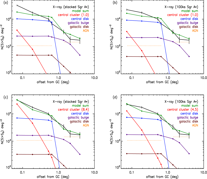
A more recent study by Schödel et al. (2007) of the stellar population and mass content in the Galactic nucleus shows evidence for a higher mass contained in the central 1 pc than predicted by studies and they speculate the excess may be due to a stellar remnant population such as black holes. Fig. 6 shows the composition of the stellar components (, , & ) in comparison with the observed projected X-ray source density. Fig. 6a shows the fit results using the stacked Sgr A* data (the same as Fig. 5b) and Fig. 6b for the 100 ks Sgr A* data. In order to allow the possible excess of the X-ray population in the Galactic nucelus relative to the observable stellar population, we also fit the X-ray distribution by freeing the relative normalization parameter of the central spherical cluster component () with respect to the rest of the components (c & d in Fig. 6). The resulting fits are substantially better, but they require a large excess of the central stellar cluster component relative to the fixed normalization given in Section 4.3: 8.4 more for the stacked Sgr A* data and 4.5 more for the 100 ks observation. This excess is still larger than the mass excess ( 2) of the nucleus above the observable stellar cluster estimated by Schödel et al. (2007), although the latter has a large uncertainty (%).
5.2. Total Surface Brightness
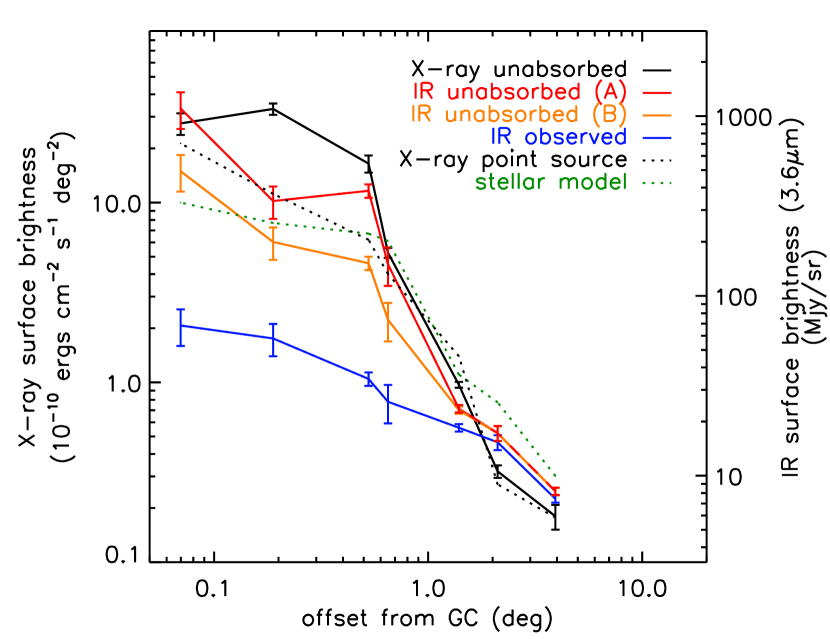
Since the IR surface brightness is a good indicator of the stellar population, a direct comparison of the IR and X-ray surface brightness provides an independent clue on the origin of the X-ray emission in the fields without influence of the uncertainties in the stellar model. In Table 5 we list the total X-ray and IR surface brightness of the seven fields. In Fig. 7 we compare the total IR surface brightness with the X-ray surface brightness after removing the contribution from the cosmic X-ray background (CXB). The CXB is expected to be ergs cm-2 s-1 deg-2 for the Windows fields and ergs cm-2 s-1 deg-2 for the rest (Hickox & Markevitch, 2006). For easy comparison, Fig. 7 also overlays the distributions of the X-ray source density and what the stellar model predicts without the AGN component in the dotted lines.
The X-ray surface brightness is calculated from the integrated counts in the band, using the quantile averaged model spectra of the group for the Windows fields and the group for the rest (Table 3). In order to subtract the instrumental background, we use the CXC background database constructed from stowed observations. For the relative normalization of the background subtraction, we use the the integrated counts in the 10.5 - 12.5 keV. The error bars in Fig. 7 are the quadratic sum of the statistical and systematic errors and the errors of the CXB estimates. For the statistical errors, we use the difference in the flux estimates between the PL and PL+Fe models.
The IR surface brightness is calculated from the 3.6 m mosaic images (1.2″pixel) generated by Galactic Legacy Infrared Mid-Plane Survey Extraordinaire (GLIMPSE) from the Spitzer/IRAC observations (Churchwell et al., 2009). The error is based on the statistical variation of the surface brightness in the four Chandra ACIS-I FoVs of each field. In order to estimate the unabsorbed surface brightness consistently with the X-ray flux estimates, we assume the estimates by the quantile analysis in Table 3 ( for the Windows fields and for the rest). We use the estimates by both models (line A for PL and line B for PL+Fe in Fig. 7) to explore the dependence of the estimates. For a given estimate, we use , , and (Nishiyama et al., 2009).
The radial distribution of the CXB-subtracted X-ray surface brightness roughly matches with the distribution of the unabsorbed IR surface brightness under the given uncertainties with the possible exception of the Arches field. This indirectly supports the idea that they share a common origin. In particular, the distribution of the unabsorbed IR surface brightness matches with the X-ray source distribution, showing higher concentration at the GC than the stellar distribution model. The origin of the discrepancy between the stellar distribution model and the IR surface brightness is unclear and requires further investigations, but note that the unabsorbed IR brightness in the high extinction fields depends sensitively on the extinction estimates, resulting in relatively large uncertainties. This dependence is also evident in the large variation among the ACIS-I FoVs in each field, which is at least in part due to the variation in the extinction across the FoVs. The radial distributions of the total X-ray surface brightness (Fig. 7) and the X-ray source density (Fig. 5) also shows a slightly different trend in a few fields such as the Arches field. For instance, the difference in the Arches field is due to the large contribution of a few bright sources in the total flux. We will address the detail of the unresolved X-ray emission with respect to the identified point sources in a following paper (Hong et al., 2009b).
5.3. Comparison with other results
According to Eq. 5 in M03, the X-ray source density in the Sgr A* field is 0.60 0.04 X-ray sources arcmin-2 at ergs cm-2 s-1 or ph cm-2 s-1 in the 2–8 keV range under their assumption of a power law spectrum with and cm-2 111111M06 assume for the X-ray spectra of the sources in the region around the GC. This is roughly consistent with our results, 0.86 0.17 arcmin-2 at ergs cm-2 s-1 from the stacked results under the PL+Fe model. The error is derived from the quadratic sum of the statistical error and 20% systematic errors (the difference between the PL and PL+Fe model).
Table 6 summarizes a few estimates of the specific luminosity of the Galactic X-ray point sources in the Chandra/ACIS energy range in the literature. The range of the specific luminosity in our study is the variation among the seven fields under the assumption of the PL+Fe model for the X-ray spectra. Using Eq. 7 in M06 and assuming the values in Fig. 5a and the number density of the X-ray sources ( X-ray sources at ergs s-1) in Table 4, we get ergs s-1 in keV for the luminosity range of ergs s-1.
M06 interpreted the result in Sazonov et al. (2006, hereafter S06) to be ergs s-1 for ergs s-1 using Eq. 5 in S06 and Eq. 7 in M06, and claimed their result ( ergs s-1 ) is consistent with S06. However, the result in S06 is calculated in the 2–10 keV range and M06 in 0.5–8 keV. In the keV range, the result in M06 becomes ergs s-1 under their assumption of and . Similarly, the result in S06 is scaled to be ergs s-1 in the same energy band. So there is a hint of mismatch in the results between M06 and S06 if one follows the scaling in M06, but also note Fig. 9 in S06 shows ergs s-1 in the 2–10 keV band for ergs s-1, which is consistent with M06 and lower than the scaling done for S06 in M06. This conversion also reveals the result in M06 is consistent with our result for the Sgr A* field. Using a similar scaling based on Eq. 5 in S06, we get ergs s-1 for the X-ray emissivity reported by Revnivtsev, Vikhlinin & Sazonov (2007, hereafter R07b) in the keV range for ergs s-1, assuming 3% of tht total emission in the same luminosity range based on Fig. 6 in R07b. Due to many different underlying assumptions in the above estimates (e.g. the spectral model parameters, stellar models, etc), it is not easy to make a fair comparison among the reported results. The large uncertainties make these results appear consistent within 2, but our results are at the lower end of these findings.
M06 and Muno et al. (2008, hereafter M08) have presented the X-ray source distribution in a region around the GC. In the case of the log-log distribution, one of the interesting results in M06 and M08 is a flatter distribution of the X-ray sources in the Arches Cluster and the subsequent excess of the X-ray sources near the high end of the flux range, compared to the Sgr A* field. We also see a similar cross over between the unstacked Sgr A* field and the Arches Cluster at ergs cm-2 s-1 (or at ergs cm-2 s-1 with the stacked Sgr A field, out of the range in the Fig. 5a). We believe this is a simple statistical fluctuation rather than a true representative of the population, arising from a small number of sources in the narrow FoV, where a few strong sources ( in the Arches Cluster) skew the shape of the whole distribution. In fact, the small number statistics is also evident in the jumpy shape of the distributions near the high end of the flux range. In Fig. 5 of M06, the excess of the X-ray sources in the Arches Cluster above ph cm-2 s-1 is boosted by excluding the overlapping region between the Sgr A* field and the Arches Cluster from the sky coverage calculation for the X-ray sources of the Arches Cluster. In order to minimize the effects due to the small number statistics, in our analysis, we focus on the solid line section of the distributions that contain at least 10 or more sources. In addition, quantile analysis results in a slightly higher value (%) of the rate-to-flux conversion factor for the sources in the Sgr A* field than the same for the Arches Cluster (see Fig. 4), which in turn pushes the log-log distribution of the Sgr A* field relatively higher. As a result, we find the slopes of the log-log distributions of the Arches Cluster and Sgr A* fields are consistent and the Sgr A* field contains more X-ray sources than the Arches Cluster consistently below ergs cm-2 s-1.
In the case of the radial distribution, the excess of the X-ray sources in the Sgr A* field with respect to the stellar model is about 3 above the stellar model if one considers both the statistical errors and the systematic errors in the flux estimates (about 10 above only with the statistical errors). M08 find about 2.5 excess of the X-ray sources at the GC compared to the best fit stellar model.
5.4. Another source population in Sgr C (or Sgr B2)?
The distribution is roughly consistent with the observed radial distribution of the X-ray sources in the GB fields within 2–3 except for the Sgr C field. The distribution is a merely empirical outcome if the observed X-ray source density consists of multiple components. On the other hand, the apparent distribution along with the similar X-ray spectral properties may imply that the GB X-ray population belongs to a homegenous component. If true, the excess of the Sgr C and Sgr B2 fields can be simply viewed as the presence of another source population in these fields in addition to the population following the distribution. The Sgr C field, like the Sgr B2 field, contains molecular HII complexes that host massive star formation. These molecular clouds are very luminous in hard X-rays, in particular with the 6.4 keV neutral iron line (Murakami et al., 2001a, b). In our analysis, the estimates of the value in the PL and PL+Fe model for the stacked spectra of the sources in the Sgr B2 and C fields, are relatively lower compared to the rest of the fields, suggesting the possibility of another source population with a different spectral type that could be related to the star formation.
6. Conclusion and Future Work
In the log-log distribution of the sources in the GB fields, the systematic errors arising from certain assumptions of spectral type is usually disregarded due to lack of alternative approaches. However they often dominate other systematic errors such as the EB, completeness or even statistical errors. The quantile analysis allows for a simple, robust method to assign a proper spectral type for flux calculation. The technique is shown to be reliable in the hard band ( keV) and insensitive to selection of the spectral model. In the soft band ( keV), where the Galactic extinction has a great influence in the spectra, the result can vary drastically depending on the assumed spectral model class. Therefore, any results covering the soft energy range should be taken with caution.
The log-log and radial distribution of the GB fields including the three low extinction Windows show the high concentration of the GB X-ray sources near the GC. The GB distribution clearly extends out to 1.4∘ (LW) from the GC and possibly more. The spectral type of the GB X-ray sources appears to be largely consistent across the region under the power law model with an iron emission line at 6.7 keV. It is possible that one type of source constitutes the majority of the GB population, and the estimated X-ray density is consistent with the majority being magnetic CVs (IPs). The relation of the radial distribution of the X-ray sources appears to be simply empirical in comparison with the stellar model compositions. Since the gravitational influence of the central supermassive black hole is only dominant within a few central pc (a few arcmin) at most, there is no compelling physics behind the relation being fundamental out to a few degrees from the GC. However, the discrepancy between the stellar models and the X-ray distribution, and the apparent homogeneity of the X-ray spectral properties of these X-ray sources pose other possibilities: the relation may not be so empirical or at least the X-ray source population contains some components that are not easily traceable by the visible stellar population.
The radial distributions of the total X-ray and IR surface brightness in the fields match within the given uncertainties, implying the same origin. The radial distribution of the IR surface brightness resembles the distribution of the X-ray point sources perhaps better than predicted by stellar distribution models, but a further detailed analysis is required because of the sensitive dependence of the IR surface brightness on the extinction estimates in the high extinction fields. In the case of the X-ray surface brightness, the additional care must be taken due to dominant contributions of a few bright sources on the X-ray flux in star formation fields such as The Arches field.
While multiwavelength observational campaigns provide important clues on the GB X-ray population, the true nature of the nature of GB X-ray sources may not be completely resolved due to source confusion and high obscuration. A deep observation ( Ms) of the LW (Revnivtsev et al, 2009), designed to investigate the nature of the Galactic Ridge X-ray emission (GRXE) in the field, is very encouraging for studies of the nature of X-ray point sources in the GB. Such a deep observation allows a direct detection of iron emission lines or X-ray variability in many of the GB X-ray sources, with which we can identify the nature of individual sources. We note only a handful of sources in the 1 Ms data of the Sgr A* field had enough statistics for identification through such a direct discovery (M03,M04). But the low extinction in the Window fields can be a game changer. For instance, we have identified an IP in the BW from the 100 ks observation, based on the periodic X-ray modulation associated with the X-ray spectral change (Hong et al., 2009a). According to its average flux, the source can be a bright IP ( 1033 ergs s-1) near the GC, but for a similar source in the Sgr A* field it would be very difficult to observe such a spectral change or periodic modulation due to the heavy absorption. By a crude scaling based on one IP found in the 100 ks observation of the BW, one can expect about 30 to 40 such identifications in a 1 Ms exposure of the BW121212Assume the identifiable source distribution is proportional to , where gets 10 times fainter, and also assume an additional 20-30% increase in the probability of catching highly variable X-ray sources based on the difference in the stacked and unstacked data set of the Sgr A* field.. Such findings would also provide enough statistics to explore the radial distribution of this particular source type. Therefore, continuous X-ray monitoring of the low extinction Window fields including the SW and BW is another important approach for unveiling the nature of the GB X-ray sources. Note that the Window fields are also suitable for searching non-magnetic CVs in the GB. These are potentially more abundant than magnetic CVs, but they are known to have relatively soft spectra and thus they would be likely hidden in the high extinction fields such as the Sgr A* field.
This work is supported in part by NASA/Chandra grants GO6-7088X, GO7-8090X and GO8-9093X. We thank the referee for the insightful comments and discussions.
References
- Ak et al. (2008) Ak, T., et al., 2008, New Astronomy, 13, 133.
- Baganoff et al. (2003) Baganoff, F. K. et al. 2003, ApJ, 591, 891.
- Bogdanov et al. (2005) Bogdanov, S., Grindlay, J. E., & van den Berg, M., 2005 ApJ, 630, 1029.
- Cappelluti et al. (2005) Cappelluti, N. et al. 2005, ApJ, 430, 39.
- Churchwell et al. (2009) Churchwell, E. et al. 2009, PASP, 121, 213.
- Drimmel et al. (2003) Drimmel, R., Cabrera-Lavers, A., & Lopez-Corredoira, M., 2003, ApJ, 409, 205.
- Ebisawa et al. (2005) Ebisawa, K., et al. 2005, ApJ, 635, 214.
- Freeman et al. (2002) Freeman, P.E. et al. 2002, ApJS, 138, 185.
- Gehrels et al. (1986) Gehrels, N. et al. 1986, ApJ, 303, 336.
- Grindlay et al. (2005) Grindlay, J.E. et al. 2005, ApJ, 635, 907.
- Grindlay et al. (2009) Grindlay, J.E. et al. 2009, in preparation.
- Heinke et al. (2008) Heinke, C. O., et al., 2008 AIPC, 1010, 136.
- Hickox & Markevitch (2006) Hickox, R. C. & Markevitch, M., 2006 ApJ, 645, 95.
- Hong et al. (2004) Hong, J, Schlegel, E. M. & Grindlay, J. E., 2004, ApJ, 614, 508. (H04)
- Hong et al. (2005) Hong, J, et al. 2005, ApJ, 635, 907. (H05)
- Hong et al. (2009a) Hong, J, et al. 2009a, ApJ, 699, 1053.
- Hong et al. (2009b) Hong, J, et al. 2009b, in preparation
- Kim et al. (2004) Kim, D.-W. et al. 2004, ApJS, 150, 19.
- Kim et al. (2007) Kim, E. et al. 2007, ApJ, 659, 29
- Kent et al. (1991) Kent, S. M., Dame, T. M., & Fazio, G. 1991, ApJ, 378, 131
- Launhardt et al. (2002) Launhardt, R., Zylka, R., & Mezger. P. G. 2002, A&A, 384, 112
- Laycock et al. (2005) Laycock, S. et al. 2005, ApJL, 634, 53 (L05)
- Liu & Li (2006) Liu, X. W. & Li, X. D. 2006 AA, 449, 135.
- Muno et al. (2003) Muno, M. P. et al. 2003, ApJ, 589, 225 (M03)
- Muno et al. (2004) Muno, M. P. et al. 2004, ApJ, 613, 1179 (M04)
- Muno et al. (2005) Muno, M. P. et al. 2005, ApJ, 633, 228
- Muno et al. (2006) Muno, M. P. et al. 2006, ApJS, 165, 173 (M06)
- Muno et al. (2008) Muno, M. P. et al. 2008, submitted to ApJ, astro-ph/0809.1105
- Murakami et al. (2001a) Murakami, H. et al. 2001a, ApJ, 550, 297
- Murakami et al. (2001b) Murakami, H. et al. 2001b, ApJ, 558, 687
- Nishiyama et al. (2009) Nishiyama, S. et al. 2009, ApJ, 696, 1407
- Oh, Kim & Figer (2009) Oh, S., Kim, S & Figer. D. F. 2009, arXiv:0906.0765
- Picaud & Robin (2004) Picaud, S. &, Robin. A. C. 2004, A&A, 417, 651
- Pretorius et al. (2007) Pretorius, M. L. et al. 2007, MNRAS, 382, 1279
- Ramsay & Cropper (2004) Ramsay, M. & Cropper, M. 2004, MNRAS, 347, 497.
- Revnivtsev & Sazonov (2007) Revnivtsev, M. & Sazonov, S., 2007a A&A, 471, 159.
- Revnivtsev, Vikhlinin & Sazonov (2007) Revnivtsev, M., Vikhlinin, A. & Sazonov, S., 2007b A&A, 473, 857 (R07b).
- Revnivtsev et al (2009) Revnivtsev, M., 2009, Nature, 458, 1142
- Ritter & Kolb (2003) Ritter H., Kolb U. 2003, A&A, 404, 301 (update RKcat7.10).
- Robin et al. (2003) Robin, A. C. et al., 2003, A&A, 409, 523.
- Ruiter et al. (2006) Ruiter, A., Belczynski, K. & Harrison, T. 2006, ApJL, 640, 167 (R06).
- Sakano et al. (2005) Sakano, M. et al. 2005, MNRAS, 357, 1211.
- Sazonov et al. (2006) Sazonov, S. et al. 2006, A&A, 450, 117 (S06).
- Schlegel et al. (1998) Schlegel, D., Finkbeiner, D. & Davis, M., 1998, ApJ, 500, 525.
- Schödel et al. (2007) Schödel, R., et al., 2007, A&A, 469, 125.
- Stanek (1998) Stanek, K. Z. 1998, Astro-ph/9802307
- van den Berg et al. (2006a) van den Berg, M. et al. 2006a, ApJL, 135, 647
- van den Berg et al. (2009) van den Berg, M. et al. 2009, submitted to ApJ.
- Wang et al. (2002) Wang, Q. D. , Gotthelf, E. V. & Lang, C. C., 2002, Nature, 415, 148.
- Wang et al. (2006) Wang, Q. D. , Dong, H. & Lang, C., 2006, ApJ, 371, 38 (W06).
- Wijnands et al. (2005) Wijnands, R., et al. 2005, ApJ, 618, 883
| Field | Obs. ID | aOffset | b | cGTI | Source countd | |||||
|---|---|---|---|---|---|---|---|---|---|---|
| (∘) | (∘) | (∘) | (ks) | Combined | ||||||
| BW | 3780 | 1.06 | 3.83 | 3.93 | 0.31 | 96 | 365 | 326 | 134 | 407 |
| SW | 4547, 5303 | 0.25 | 2.15 | 2.12 | 0.48 | 96 | 388 | 313 | 140 | 433 |
| LW | 5934, 6362,6365 | 0.10 | 1.43 | 1.39 | 0.68 | 94 | 282 | 184 | 174 | 319 |
| Sgr B2 | 944 | 0.59 | 0.03 | 0.65 | 81.2 | 97 | 279 | 126 | 224 | 363 |
| Sgr C | 5892 | 0.57 | 0.02 | 0.51 | 52.7 | 97 | 313 | 188 | 241 | 442 |
| Arches | 4500 | 0.12 | 0.02 | 0.19 | 52.5 | 97 | 330 | 84 | 328 | 423 |
| Sgr A* | 3665 | 0.06 | 0.05 | 56.5 | 88 | 401 | 92 | 400 | 508 | |
| (Stackede) | 698 | 2251 | 370 | 2316 | 2876 | |||||
(a) The aim point offset from Sgr A*. (b) The estimates for the integrated neutral hydrogen column density along the line of the sight (in cm-2) by Schlegel et al. (1998) for the location of the aimpoint. This is only for guiding purpose due to the large uncertainty in the Galactic plane fields. (c) The good time intervals (GTIs). The total exposure (i.e. before cleaning) is 100 ks each (750 ks for the stacked Sgr A* field). (d) The number of the sources with net count in the broad band (0.3–8 keV) on the ACIS-I CCDs (0, 1, 2, and 3) in the three detection bands (: 0.3–8 keV, : 0.3–2.5 keV, : 2.5–8 keV) and the combined unique source list. (e) 14 pointings are stacked, and they are Obs. ID 242, 2951, 2952, 2953, 2954, 2943, 3663, 3392, 3393, 3549, 3665, 4683, 4684 and 5360.
| Source | Posi. | Net countsc | d | Quantiles | Unabsorbed Fluxf | ||||||||
| Name | Field | R.A. | Dec. | Errora | Offsetb | Quartile | Group | ||||||
| (CXOPS J) | (∘) | (∘) | (″) | (′) | (keV) | Ratioe | ( ergs cm-2 s-1) | ||||||
| 180230.4-295647 | BW | 270.626934 | -29.946497 | 1.29 | 10.05 | 123.6 (14.3) | 71.5 (10.9) | 53.3 (9.9) | 5.4 | 1.89 (0.10) | 1.30 (0.17) | 1 | 1.31 (0.24) |
| 180231.2-295528 | BW | 270.630007 | -29.924698 | 2.37 | 10.12 | 38.6 (10.9) | 4.6 (6.9) | 34.8 (8.9) | 3.9 | 3.56 (0.29) | 1.68 (0.30) | 3 | 1.12 (0.29) |
| 180235.9-295323 | BW | 270.649946 | -29.889846 | 3.32 | 9.87 | 23.6 (9.6) | 23.4 (8.1) | -0.2 (5.6) | 0.0 | 1.05 (0.15) | 2.08 (0.48) | 1 | -0.01 (0.13) |
| …. | |||||||||||||
| 175404.4-294359 | SW | 268.518385 | -29.733089 | 2.56 | 9.58 | 34.1 (11.2) | 25.3 (9.2) | 5.9 (6.6) | 0.9 | 1.34 (0.18) | 1.63 (0.64) | 1 | 0.13 (0.14) |
| 175405.3-294717 | SW | 268.522117 | -29.788307 | 2.47 | 8.04 | 22.2 (8.9) | 19.7 (7.7) | 2.9 (5.1) | 0.6 | 1.40 (0.24) | 1.61 (0.40) | 1 | 0.06 (0.11) |
| 175406.7-294239 | SW | 268.527957 | -29.711050 | 1.97 | 9.99 | 42.2 (12.0) | 20.6 (9.4) | 22.5 (8.0) | 2.8 | 2.12 (0.54) | 1.08 (0.32) | 2 | 0.69 (0.24) |
| …. | |||||||||||||
| 175051.2-293418 | LW | 267.713518 | -29.571797 | 1.02 | 8.10 | 113.8 (13.8) | 36.2 (9.1) | 75.8 (10.9) | 7.0 | 2.63 (0.20) | 1.25 (0.16) | 2 | 2.21 (0.32) |
| 175052.0-293319 | LW | 267.716827 | -29.555400 | 2.92 | 8.14 | 16.4 (9.2) | 5.2 (6.8) | 9.3 (6.6) | 1.4 | 0.97 (5.31) | 0.20 (0.29) | 2 | 0.27 (0.19) |
| 175053.3-293207 | LW | 267.722097 | -29.535548 | 2.12 | 8.29 | 25.0 (10.3) | 2.8 (7.3) | 22.4 (7.8) | 2.9 | 3.46 (0.38) | 1.74 (0.48) | 3 | 0.77 (0.27) |
| …. | |||||||||||||
Notes.—This table shows a part of the complete
list, which is available in the electronic edition.
(a) The 95% positional error radius.
(b) The offset from the aim point.
(c) The net counts based on the aperture photometry(Hong et al., 2005).
(d) The signal to noise ratio in the band. The sources with are
included in the log-log plot in Fig. 5.
(e)
(f) Based on the PL+FE model using quantile analysis. We do
not include the flux estimates in the other bands due to their large
uncertainty. See the text for the details.
The uncertainties for net counts and fluxes are statistical errors.
| Quartile | PL from | PL+Fe (He-) from | PL (+Fe He-) from | |||||||
| Field | Ratioa | Quantile Diagramb | Quantile Diagramc | Spectral Model Fitd | ||||||
| EWe | /DoFf | |||||||||
| (keV) | ( cm-2) | ( cm-2) | ( cm-2) | (keV) | ||||||
| unabsorbed hard sources () | ||||||||||
| BW | 1.97(2) | 1.02(1) | 1.38(03) | 0.31(03) | 1.42(03) | 0.32(05) | 1.36(2) | 0.26(01) | 0.15(9) | 113.3/167 |
| SW | 2.10(5) | 1.03(2) | 1.35(07) | 0.37(06) | 1.38(10) | 0.38(08) | 1.22(3) | 0.25(03) | g | 48.7/69 |
| LW | 2.66(4) | 1.09(2) | 1.28(07) | 0.73(09) | 1.35(07) | 0.79(09) | 0.99(2) | 0.38(02) | g | 125.9/148 |
| absorbed hard sources () | ||||||||||
| BW | 3.22(13) | 1.38(9) | 1.66(37) | 2.20(70) | 1.74(37) | 2.30(70) | 1.22(4) | 1.66(16) | g | 24.8/26 |
| SW | 3.39(7) | 1.52(4) | 1.77(23) | 2.90(50) | 1.91(23) | 3.10(50) | 1.58(4) | 2.78(19) | g | 35.4/22 |
| LW | 3.48(5) | 1.43(3) | 1.21(10) | 1.95(15) | 1.32(10) | 2.10(20) | 1.30(2) | 1.89(06) | 0.17(8) | 93.1/115 |
| Sgr B2 | 4.75(4) | 1.86(2) | 0.37(14) | 3.40(80) | 0.25(17) | 5.70(90) | 0.50(1) | 6.20(22) | 0.61(7) | 105.2/154 |
| Sgr C | 4.81(3) | 1.90(2) | 0.26(10) | 4.8(1.0) | 0.46(21) | 7.8(1.2) | 0.10(1) | 3.95(18) | 0.38(5) | 172.3/189 |
| Arches | 4.54(2) | 1.83(1) | 0.14(07) | 4.00(50) | 0.67(14) | 5.70(70) | 0.85(1) | 5.17(12) | 0.66(5) | 319.4/363 |
| Sgr A* | 4.69(2) | 1.91(1) | 0.31(14) | 6.40(60) | 0.94(14) | 9.00(80) | 1.02(1) | 6.95(12) | 0.46(4) | 324.3/364 |
(a) (b) The parameter estimates based on quantile analysis for a power law model. (c) The same as (b) but with a fixed 0.4 keV EW at 6.7 keV (d) The parameter estimates by the spectral model fit. (e) the EW of 6.7 keV line. (f) Degrees of Freedom. (g) Due to poor statistics, the spectral fit is done with a power law model without an iron line. See §4.
| X-ray Sourceb | Stellar Model Ac | Stellar Model Bd | ||||||
| Surface | Volume | Star volume | Star surface | X-ray to | X-ray | Required CV | Star volume | |
| Field | density | density | density | mass density | stellar mass | to stars | to starse | density |
| (deg-2) | (10-7 pc-3) | (pc-3) | (108 deg-2) | (10-7) | (10-7) | (10-5) | (pc-3) | |
| Field to field Comparison | ||||||||
| BW | 25(45) | 3.2(5.7) | 2.1 | 0.5 | 5.1(9.1) | 1.6(2.8) | 2.6(4.6) | 3.2 |
| SW | 39(47) | 4.9(6.0) | 5.3 | 1.3 | 3.1(3.7) | 0.9(1.1) | 1.6(1.9) | 6.7 |
| LW | 203(64) | 25(8.1) | 7.6 | 1.8 | 11(3.5) | 3.4(1.1) | 5.6(1.8) | 8.3 |
| Sgr B2 | 582(93) | 73(11) | 41 | 10 | 5.7(0.9) | 1.8(0.3) | 2.9(0.5) | 8.8 |
| Sgr C | 902(113) | 113(14) | 45 | 11 | 8.1(1.0) | 2.5(0.3) | 4.1(0.5) | 8.9 |
| Arches | 1624(153) | 204(19) | 52 | 13 | 12(1.2) | 3.9(0.4) | 6.5(0.6) | 9.1 |
| Stacked Sgr A* | 3100(187) | 389(23) | 68 | 17 | 18(1.1) | 5.7(0.3) | 9.5(0.6) | 9.1 |
| 100 ksSgr A* | 2117(176) | 266(22) | 68 | 17 | 12(1.1) | 3.9(0.3) | 6.5(0.5) | 9.1 |
| By the fit to the radial distributionf | ||||||||
| with stacked Sgr A* (Fig. 5b or 6a) | 10.3(0.5) | 3.2(0.2) | 5.3(0.3) | |||||
| with 100ks Sgr A* (Fig. 6b) | 9.2(0.5) | 2.8(0.2) | 4.7(0.3) | |||||
| By the fit with the freed relative normalization of g | ||||||||
| with stacked Sgr A* (Fig. 6c) | 7.1(0.6) | 2.2(0.2) | 3.6(0.3) | |||||
| with 100ks Sgr A* (Fig. 6d) | 7.5(0.6) | 2.3(0.2) | 3.8(0.3) | |||||
(a) Assumes the hard X-ray sources ( ergs cm-2 s-1 in ) or stars seen within the FoV are mainly ( 80%) from 6–10 kpc distance. (b) Using the PL+Fe model. We subtract the expected AGN numbers, 145 deg-2 from the Window fields and 107 deg-2 from the high extinction fields. (c) The composite model in M06 and references therein. The model gives the stellar mass density in the unit of pc-3, and we assume the local value of 0.144 stars pc-3 and 0.04 pc-3 to get the star number density (Robin et al., 2003). This relation should be good for the bulge in the case of CVs and active binaries, but perhaps not good for young stars (Sazonov et al., 2006). (d) The stellar density model by Picaud & Robin (2004) for the Galactic disk and outer Galactic bulge. The model does not include a central nucleus, so the (italic) values for the Sgr B2, Sgr C, Arches, and Sgr A* fields are not reliable. See §5.1. (e) The required CV to star density to explain the hard GB X-ray sources by IPs. We assume that IPs are 5% of all CVs (e.g. 2–8% in R06) and that about 12% of them are detected above ergs s-1 (e.g. 10–16% in R06), which corresponds ergs cm-2 s-1 for the sources near the GC (see text). (f) The relative normalizations among stellar model components are fixed as given in Section 4.3. (g) The relative normalization of the central spherical cluster component of the stellar distribution is allowed as a free parameter and fitted as well.
| X-raya | IR | ||||
|---|---|---|---|---|---|
| Field | 2–8 keV (the band) | 3.6 m | |||
| (10-10 ergs cm-2 s-1 deg-2) | (MJy/sr) | ||||
| PL | PL+Fe | observed | unabsorbed (PL)b | unabsorbed (PL+Fe)c | |
| BW | 0.34(0.02) | 0.35(0.02) | 7.4(0.4) | 8.2(0.4) | 8.2(0.4) |
| SW | 0.48(0.01) | 0.49(0.01) | 15(1) | 17(2) | 17(2) |
| LW | 1.10(0.01) | 1.13(0.01) | 18(1) | 24(1) | 24(1) |
| Sgr B2 | 5.09(0.05) | 5.42(0.05) | 26(6) | 74(18) | 150(36) |
| Sgr C | 14.9(0.1) | 16.6(0.1) | 35(3) | 152(13) | 384(33) |
| Arches | 30.9(0.1) | 33.4(0.1) | 58(12) | 199(40) | 337(69) |
| Sgr A* | 23.93(0.02) | 27.72(0.02) | 68(16) | 493(110) | 1100(250) |
(a) Assume the spectral model using the group for the Windows field and the group for the rest in Table 3. The error is of the statistical origin. Note the expected cosmic X-ray background (CXB) is ergs cm-2 s-1 deg-2 for the Windows fields and ergs cm-2 s-1 deg-2 for the rest (Hickox & Markevitch, 2006). See the §5.2. (b) The estimate by PL (line B in Fig. 7). (c) The estimate by PL+Fe (line A in Fig. 7).
| Energy | Luminosity | Scaled for | |||
|---|---|---|---|---|---|
| Source | Reported | Range | Range | ergs s-1 in 2–8 keV | Studied Fields |
| ( ergs s-1 ) | (keV) | (ergs s-1) | ( ergs s-1 ) | ||
| This Study | 0.5 – 2.8 | 2–8 | 0.5 – 2.8 | 7 GB fields (100 or 750 ks) | |
| M06 | 5.0 2 | 0.5–8 | 3.3 1.3 | around the GC (100 or ks ) | |
| S06 | 45 9 | 2–10 | 9 3 a | the local solar neighborhood | |
| 6 2 b | |||||
| R07b | 77 39 | 2–10 | 3 1 c | the Sgr A* field (1 Ms) |