SHEP 09-16

On discrete Minimal Flavour Violation
Roman Zwicky ^a and Thomas Fischbacher ^b
a School of Physics & Astronomy

^b School of Engineering

University of Southampton

Highfield, Southampton SO17 1BJ, UK

We investigate the consequences of replacing the global flavour symmetry of Minimal Flavour Violation (MFV) $SU(3)_{Q}\times SU(3)_{U}\times SU(3)_{D}\times..$ by a discrete ${\cal D}_{Q}\times{\cal D}_{U}\times{\cal D}_{D}\times..$ symmetry. Goldstone bosons resulting from the breaking of the flavour symmetry generically lead to bounds on new flavour structure many orders of magnitude above the TeV-scale. The absence of Goldstone bosons for discrete symmetries constitute the primary motivation of our work. Less symmetry implies further invariants and renders the mass flavour basis transformation observable in principle and calls for a hierarchy in the Yukawa matrix expansion. We show, through the dimension of the representations, that the (discrete) symmetry in principle does allow for additional $\Delta F=2$ operators. If though the $\Delta F=2$ transitions are generated by two subsequent $\Delta F=1$ processes, as for example in the Standard Model, then the four crystal-like groups $\Sigma(168)\thickapprox{\rm PSL}(2,\mathbb{F}_{7})$, $\Sigma(72\varphi)$, $\Sigma(216\varphi)$ and especially $\Sigma(360\varphi)$ do provide enough protection for a TeV-scale discrete MFV scenario. Models where this is not the case have to be investigated case by case. Interestingly $\Sigma(216\varphi)$ has a (non-faithful) representation corresponding to an $A_{4}$-symmetry. Moreover we argue that the, apparently often omitted, $(D)$-groups are subgroups of an appropriate $\Delta(6g^{2})$. We would like to stress that we do not provide an actual model that realizes the MFV scenario nor any other theory of flavour.

1 Introduction

In the absence of Yukawa interaction, $G_{F}=U(3)^{5}=U(3)_{Q}\times U(3)_{U_{R}}\times U(3)_{D_{R}}\times U(3)_{L}\times U(3)_{E_{R}}$ is the maximal global symmetry that commutes with the gauge groups of the Standard Model (SM) [1]. The Yukawa matrices $Y_{U,D,E}$ break this symmetry down to

$$G_{F}=U(3)^{5}\stackrel{{\scriptstyle Y_{U,D,E}}}{{\longrightarrow}}U(1)_{B}\times U(1)_{L}\;.$$ (1)

It was realized a long time ago [3] that these sort of flavour symmetries forbid flavour changing neutral currents (FCNC) at tree level. Most models of new physics do not posses a rigid flavour structure and large FCNC effects should be expected in general. On the other hand experiments in the quark flavour sector CLEO, BaBar, Belle, NA48, KTeV, KLOE, TeVatron, .. do not, yet, show any significant deviations of FCNC or CP-violation. This motivated the effective field theory approach, called Minimal Flavour Violation (MFV) [4], where it is postulated that the sole sources of flavour violation are the Yukawa matrices. We shall be more precise later on. New physics contributions of the MFV-type compared to the SM in $K_{0}$ and $B_{d}$ oscillations can in principle still be as large as $C_{\rm SM}/C_{\rm MFV}\simeq(0.5\,\mbox{TeV})^{2}/m_{W}^{2}$ [4]. It is the size of the Wilson coefficient $C_{\rm MFV}$, including its implicit loop suppression factor, what we refer to as “TeV-scale MFV scenario”. The extension of the concept from the quark sector to the lepton sector depends on the nature of the neutrino masses [6]. For notational simplicity we shall focus in this work on the quark sector. The results can easily be transfered to the lepton sector.

Even in the absence of the knowledge of the exact dynamics one delicate question might be raised: How is the $G_{F}$ symmetry broken? If the symmetry is broken spontaneously at some scale $\Lambda_{F}$, then this gives rise to $3\cdot 8+2=26$ CP-odd massless Goldstone bosons associated with the breaking of $U(3)^{3}\to U(1)_{B}$. In connection with non-abelian family symmetries such Goldstone bosons are known as familons [8]; they are formally similar to an axion arising from the breaking of an axial U(1)-symmetry. Due to the fact that they are Goldstone bosons their interactions with SM fields take on the universal form ${\cal L}_{\rm eff}\sim\frac{1}{\Lambda_{F}}\bar{D}_{L}T^{a}\gamma_{\mu}D_{L}\partial^{\mu}\phi_{F}^{a}$, where $\phi_{F}^{a}$ is a familon and $T^{a}$ is the generator of the broken global symmetry. The breaking scale$\Lambda_{F}$ is subjected to experimental constraints. Focusing on $s\to d$ transitions, which would give rise to the lowest scale in a scenario of sequential symmetry breaking [7], the scale $\Lambda_{F_{\rm ds}}$ is bounded from the processes $K^{+}\to\pi^{+}\bar{\nu}\nu$. The latter competes with $K^{+}\to\pi^{+}\phi_{F_{\rm ds}}$ since the familon $\phi_{F_{\rm ds}}$ escapes detection due to its weak coupling to matter and ${\cal L}_{\rm eff}\simeq\frac{1}{\Lambda_{F_{\rm ds}}}\bar{s}_{L}\gamma_{\mu}d_{L}\partial^{\mu}\phi_{F_{\rm ds}}$, so that the bound $\Lambda_{F_{\rm ds}}>10^{8}\,\mbox{TeV}$ is rather high [10]. The relation of this scale to the MFV-scale, which is roughly bounded $\Lambda_{\rm MFV}\geq 0.5\;{\rm TeV}$ from MFV-type operators [4], is a model dependent question. If the breaking of flavour symmetry is decoupled from a lower physics scale, associated with the stabilization of the Higgs mass for example, then the bounds do not directly apply. An example is a SUSY-GUT scenario, where it is assumed that flavour is generated or broken at some high scale and resides in so-called soft terms. Then operators of the MFV-type are generated when supersymmetry is broken and the MFV-scale is associated with the SUSY scale rather than $\Lambda_{F_{\rm ds}}$. Summarizing, the dynamics of spontaneous symmetry breaking suggests that in a (continuous) MFV-scenario the generation of flavour are outside (current) experimental reach. As argued above this does not exclude the observation of novel flavour effects due to an additional sector such as SUSY-GUT.

In this paper we aim to ameliorate this situation by replacing $G_{F}$ by a discrete symmetry. Spontaneous breaking of discrete symmetries do not lead to Goldstone bosons e.g. [12]. The absence of the latter in this framework constitutes the primary motivation of our work. The main remaining issue is then to investigate whether the reduced symmetries (or what discrete groups) do provide enough protection for a discrete TeV-scale MFV-scenario. Are the bounds on the coefficient $C_{\rm dMFV}$ in the TeV-scale range?

On the technical side this endeavour amounts to study the invariants of discrete subgroups. The reduced symmetry unavoidably leads to further invariants as compared to $G_{F}$. This bears as a consequence that the flavour-mass basis transformation will become observable. The crucial question for discrete MFV is then at what level these new invariants are coming in. In this respect we find it useful to distinguish models where $\Delta F=2$ operators arise from two $\Delta F=1$ processes, as in the SM, and those where this is not the case.

Finally we would like to stress to points. First, since we are following the effective field theory approach there is no obvious connection to the scheme of constrained MFV [18], which assumes no new operators beyond those present in the SM. Second, there is no attempt made in this paper to explain valuable textures of the Yukawa matrices, i.e. the question of what is flavour. The symmetry is solely used to ensure that the Yukawa structure gouverns all flavour transition. Our work is complementary to the field of flavour models with family symmetries, revived by recent experimental information on neutrino masses and mixing angles (PMNS matrix). Those models often involve discrete symmetries and extended Higgs sectors attempting to explain the origin of flavour hierarchies. For a recent review and references on the subject, with emphasis on the neutrino sector, we refer the reader to the write-up [19].

The paper is organized as follows: In section 2 we state the problem in a more precise form. Section 3 summarizes some useful facts about groups and gives an overview of the discrete SU(3) subgroups. In section 4 it is shown at what level new invariants necessarily arise and which groups have the least invariants. Section 5 deals with the physical consequences of the previous findings and proposes to distinguish flavour models according to generation mechanism of $\Delta F=2$ operators. In the epilogue we summarize our findings and reflect on the framework and its possible extensions.

2 Formulation

2.1 Minimal Flavour Violation

In the SM the quark masses and the CKM structure originate from the Yukawa Lagrangian,

$${\cal L}_{\rm Y}=\bar{Q}_{L}HY_{D}D_{R}+\bar{Q}_{L}H_{c}Y_{U}U_{R}\;+\;{\rm h.c.}\,,$$ (2)

which breaks the flavour symmetry down to $U(1)_{B}$, c.f. Eq. (1). The symbols $U_{R}$, $D_{R}$ and $Q_{L}=(U_{L},D_{L})^{T}$ denote right and left handed SU(2)_L singlets and doublets respectively of up $U=(u,c,t)$ and down $D=(d,s,b)$ quarks. The conjugate Higgs field is defined as $H_{c}=i\tau_{2}H^{*}$.

It is observed that the quark flavour symmetry,

$$G_{q}=SU(3)_{Q_{L}}\times SU(3)_{U_{R}}\times SU(3)_{D_{R}}\;,$$ (3)

can be formally restored by associating to the Yukawa matrices the following transformation properties:

$$Y_{U}\sim(\text{\bf 3},\bar{\text{\bf 3}},\text{\bf 1})_{G_{q}}\;,\qquad Y_{D}\sim(\text{\bf 3},\text{\bf 1},\bar{\text{\bf 3}})_{G_{q}}\;.$$ (4)

In fact the flavour symmetry can even be further enhanced by two U(1) factors by appropriately assigning U(1) charges to the quark fields and the Yukawa matrices. In our opinion there is some freedom in choosing them.

An effective theory constructed from the SM fields and the Yukawa matrices is then said to obey the principle of Minimal Flavour Violation [4], if the higher dimensional operators are invariant under $G_{q}$ and CP. Operators with $\Delta F=1,2$ then assume the following form [4]

$$O^{\Delta F=1^{\prime}} =(\bar{D}_{L}Y_{U}Y_{U}^{\dagger}Y_{D}\,\sigma\!\cdot\!FD_{R})\;,$$

$$O^{\Delta F=1} =(\bar{D}_{L}Y_{U}Y_{U}^{\dagger}\gamma_{\mu}D_{L})\,\bar{D}_{L}\gamma^{\mu}D_{L}\;,$$

$$O^{\Delta F=2} =(\bar{D}_{L}Y_{U}Y_{U}^{\dagger}\gamma_{\mu}D_{L})^{2}\;,$$ (5)

in the left handed $D$-sector. The symbol $\sigma\!\cdot\!F=\sigma_{\mu\nu}F^{\mu\nu}$ denotes the contracted electromagnetic tensor, $2D_{L/R}\equiv(1\pm\gamma_{5})D$ and we would like to add that notation $\Delta F=1^{\prime}$, used here, is rather non-standard. In the remainder of this paper we shall omit the explicit indication of the $\gamma$-matrices. Transitions to right handed quarks demand substitutions of the form $D_{L}\to Y_{D}D_{R}$ etc, by virtue of $G_{q}$-invariance (3,4), leading to the well-known phenomenon of chiral suppression. The operators in the $U$-sector are simply obtained by interchanging the role of the $U$ and $D$ families. Let us parenthetically note that the predictivity of MFV [4] in the $D$ sector is in large parts due to the the fact that the top is much heavier than the other $U$-quarks

$$\left(Y_{U}Y_{U}^{\dagger}\right)_{ij}=\left(V^{\dagger}{\rm diag}(y_{u},y_{c},y_{t})^{2}V\right)_{ij}\simeq y_{t}^{2}V^{*}_{3i}V_{3j}\;,$$ (6)

where $V={\cal U}_{L}^{\dagger}{\cal D}_{L}$ is the CKM matrix, resulting from the bi-unitary diagonalization of the

$$U_{L}\to{\cal U}_{L}U_{L}\;,\quad U_{R}\to{\cal U}_{R}U_{R}\;,\quad D_{L}\to{\cal D}_{L}D_{L}\;,\quad D_{R}\to{\cal D}_{R}D_{R}\;,$$ (7)

Yukawa matrices. The masses are related to the Yukawa couplings as $\sqrt{2}m_{i}=vy_{i}$ (with $v\simeq 246\,\mbox{GeV}$) and it is worth noting that in the limit of degenerate masses the GIM mechanism reveals itself through: $(Y_{U}^{\dagger}Y_{U})_{ij}\to\delta_{ij}$.

2.2 Discrete Minimal Flavour Violation

Replacing the continuous flavour symmetry with a discrete flavour symmetry requires the following additional information or assumptions:

$$a)\quad\text{The group}\quad D_{q}={\cal D}_{Q_{L}}\times{\cal D}_{U_{R}}\times{\cal D}_{D_{R}}\subset G_{q}\;,\quad{\cal D}\subset SU(3)\;,$$

$$b)\quad\text{The representation}\quad R_{3}({\cal D}_{Q_{L}})\text{ (3D irrep of families )}\;,$$

$$c)\quad\text{(possibly) Yukawa expansion}\quad Y_{U/D}\to\kappa Y_{U/D}\;,\quad\kappa\in\mathbf{R}\;,$$ (8)

Since the three families have to transform in a 3D irreducible representation (irrep) this leads us naturally to study the discrete SU(3) subgroups, which we denote by the symbol ${\cal D}$. The irrep has to be specified since some groups have more than one of them. The reduced symmetry a) leads to new invariants and therefore renders the transition matrices (7) observable. We will argue in subsection 5.1 that this gives rise to a rather anarchic pattern of flavour transitions. This can be controlled by assuming a hierarchy in the Yukawa expansion. In a perturbative-type model for example the operators with several Yukawa insertion might originate from higher dimensional operators suppressed by some high scale $\Lambda$ and could mean $\kappa\simeq v/\Lambda$ if the Yukawa assume a vacuum expectation value (VEV) around the electroweak scale. A rough but conservative estimate in subsection 5.2 indicates that for $\kappa\simeq 0.2$ $C_{\rm dMFV}$ has the same bounds as $C_{\rm MFV}$. In this paper we shall not discuss the U(1) factors, e.g. (1), any further. We can think of them as being replaced by a discrete $\mathbb{Z}_{n}$ symmetry, $D_{q}\to D_{q}\times\mathbb{Z}_{n}..$ and they do not play a role in the type of invariants we are considering. Generally the embedding could play a more subtle role. First there is freedom of embedding ${\cal D}$ into SU(3). We will discuss this issue in section 5.1 where it is argued that the obersvability of the rotation matrices (7) can be suppressed, modulo $V_{\rm CKM}$, for certain groups by a suitable embedding. Second, we would like to draw the reader’s attention to the assumption of $D_{q}$ being embedded as a direct product of the discrete SU(3) subgroups a) into $G_{q}$. We shall comment on it in the epilogue.

3 On (discrete) groups

In this section we shall first state a few useful facts about invariants, groups and representations, which is at the heart of this paper. Then we shall say a few things about the classification of discrete SU(3) subgroups.

3.1 Useful facts

Consider irreps $\{\text{\bf A},\text{\bf B},\text{\bf C},...\}$ of some group, continuous or discrete, and denote the explicit vectors of the irreps by ${\cal V}=\{a_{r},b_{s},c_{t},...\}$. By the orthogonality theorem the number of times that the identity appears in the Kronecker product, denoted by $n_{1}$,

$$\text{\bf A}\times\text{\bf B}\times\text{\bf C}\times\dots=n_{1}\,\text{\bf 1}+\dots\;,$$ (9)

is equal to the number of independent invariants

$${\cal I}_{n}={\cal I}_{n}^{rst..}\,a_{r}b_{s}c_{t}..\;,\qquad n=1\dots n_{1}\;,$$ (10)

that can be built out of the set ${\cal V}$ specified above. Throughout this paper repeated indices are thought to be summed over. It is this statement that we shall use shortly for our main result. Before going on we would like to mention another fact, peculiar to discrete groups: The number of elements of the group is equal,

$$|{\cal D}|=\sum_{i\in\text{irreps}}{\rm dim}(R_{i}({\cal D}))^{2}\;,$$ (11)

to the sum of the squared dimensions of all irreps.

3.2 Discrete SU(3) subgroups

The discrete subgroups of SU(3) were classified a long time ago [16] and further analyzed as alternatives to SU(3)_F in the context of the eightfold way [17]. Explicit representations and Clebsch-Gordan coefficients were systematically worked out in a series of papers around 1980 [22, 23], partly motivated by the usage of discrete SU(3) subgroups as an approximation to $SU(3)_{\rm colour}$ in lattice QCD; and further elaborated very recently [24, 25, 26] in the context of family symmetries. That the catalogue of [17] as compared to [16] is not complete already surfaced in the 1980 [23, 27] and has recently been discussed more systematically in a remarkable diploma thesis [28].

The discrete subgroups of SU(3) are of two kinds. The first type consist of the analogue of crystal groups of which we list here the maximal subgroups: $\Sigma(168)$, $\Sigma(360\varphi)$ and $\Sigma(216\varphi)$. The factor $\varphi$ can in general either be one or three depending on whether the center of SU(3) is divided out or not. For the maximal subgroups it is three. The second kind are the infinite sequence of groups, sometimes called “dihedral like” or “trihedral”, $\Delta(3n^{2})\thickapprox(\mathbb{Z}_{n}\times\mathbb{Z}_{n})\rtimes\mathbb{Z}_{3}$ and $\Delta(6n^{2})\thickapprox(\mathbb{Z}_{n}\times\mathbb{Z}_{n})\rtimes S_{3}$ for $n\in{\mathbb{Z}}$. The symbol “$\thickapprox$” stands for isomorphic and “$\rtimes$” denotes a semidirect product. The largest irreps of $\Delta(3n^{2})$ and $\Delta(6n^{2})$ are 3-, respectively 6-dimensional; independent of $n$. Note, for all groups the number denotes the order of the group, i.e. the number of elements. In appendix A.2.1 we argue that the $(D)$-groups recently emphasized in [28], or more precisely the six-parameter $D(n,a,b;d,r,s)$ matrix groups, are subgroups of $\Delta(6g^{2})$, where $g$ is the lowest common multiple of $n$, $d$ and $2$. We therefore do not need to discuss them separately. Further aspects of some groups and some of their invariants are discussed in the appendix A.

We would like to add that since this paper has been first published further progress has been achieved by P.Ludl [29], who showed that topologically the $(C)$ and $(D)$-groups correspond to $(C)\thickapprox(\mathbb{Z}_{n}\times\mathbb{Z}_{n^{\prime}})\rtimes\mathbb{Z}_{3}$ and $(D)\thickapprox((\mathbb{Z}_{n}\times\mathbb{Z}_{n^{\prime}})\rtimes\mathbb{Z}_{3})\rtimes\mathbb{Z}_{2}$.

4 Invariants

The study of invariants ${\cal I}$ is the main ingredient of this paper since the effective Lagrangian approach. In the absence of the knowledge of the dynamics of the underlying model the effective Lagrangian assumes the following form

$${\cal L}^{\rm eff}=\sum_{n}C^{n}_{\rm dMFV}\left({\cal I}_{n}(\text{Quarks},\text{Yukawas}\right)+h.c)\,,\qquad C^{n}_{\rm dMFV}=\frac{c_{n}}{\Lambda^{\text{dim}({\cal I}_{n})-4}}\;,$$ (12)

where the dimension of the operator (invariant) brings in a certain hierarchy in the infinite sum above. As previously mentioned the association of $C^{n}$ with the scale of new structure is generally obscured by loop factors, mixing angles and renormalization group effects. Finding the invariants is equivalent to finding the constant tensors of the symmetry group. All objects are either in a 3 or the corresponding $\bar{\text{\bf 3}}$ representation for which we write lower and upper indices, e.g.

$${\cal I}^{(m,n)}\;\sim\;{\cal I}_{\,a_{1}..a_{m}}^{\,b_{1}..b_{n}}\;,$$ (13)

as is common practice in the literature e.g. [30]. Non-constant tensors will be denoted by ${\cal T}^{(m,n)}$. In principle this tensor classification is not sufficient for our general problem since there are three different group factors (2.2). It will though prove sufficient here to contract the other indices. We therefore contract the ${\cal D}_{U_{R}}$ index and directly write

$$(\Delta_{U})_{a}^{\phantom{x}r}\equiv(Y_{U}Y_{U}^{\dagger})_{a}^{\phantom{x}r}\;,\qquad(\Delta\in{\cal T}^{(1,1)})\;.$$ (14)

We shall often drop the subscript $U$ when there is no reason for confusion. In the reminder we shall use the following notation for left handed down quarks

$$D_{L}=(d_{L},s_{L},b_{L})\to D_{i}=(D_{1},D_{2},D_{3})\;,\qquad(D_{i}\in{\cal T}^{(1,0)})\;.$$ (15)

The operators in Eq. (2.1) are associated with invariants of the form:

$${\cal I}^{(2,2)}_{n}=({\cal I}_{n})^{ab}_{rs}\,\left(\bar{D}^{r}\Delta_{a}^{\phantom{x}s}D_{b}\right)\qquad \Delta F=1^{\prime}\;,$$

$${\cal I}^{(3,3)}_{n}=({\cal I}_{n})^{abc}_{rst}\,\left(\bar{D}^{r}\Delta_{a}^{\phantom{x}s}D_{b}\right)\bar{D}^{t}D_{c}\qquad \Delta F=1\;,$$

$${\cal I}^{(4,4)}_{n}=({\cal I}_{n})^{abcd}_{rstu}\,\left(\bar{D}^{r}\Delta_{a}^{\phantom{x}s}D_{b}\right)\,\left(\bar{D}^{t}\Delta_{c}^{\phantom{x}u}D_{d}\right)\qquad \Delta F=2\;.$$ (16)

Note that there are groups where $\Delta F=2$ operators are possible with ${\cal I}^{(2,2)}$ but those structures are definitely too far away from MFV to be of any interest to us. The group $\Sigma(60)\thickapprox A_{5}$ is an example which is discussed in appendix A.1.

4.1 No 27 ! – On the necessity of new invariants at the ${\cal I}^{(4,4)}$ level

In this subsection we will present a general argument that there are necessarily further invariants for ${\cal I}^{(4,4)}$, corresponding to the generic $\Delta F=2$ transition (16), as compared to the SU(3) case. Note the $\Delta F=2$ operator (2.1) of $G_{q}$ is obtained for $({\cal I}_{1})^{abcd}_{rstu}\equiv\delta_{r}^{\phantom{x}a}\delta_{s}^{\phantom{x}b}\delta_{t}^{\phantom{x}c}\delta_{u}^{\phantom{x}d}$. The problem in Eq. (16) reduces to finding the invariants of the following Kronecker product

$$K^{\cal D_{Q_{L}}}=\left(\bar{\text{\bf 3}}\times\text{\bf 3}\times\bar{\text{\bf 3}}\times\text{\bf 3}\right)_{s}\times\left(\bar{\text{\bf 3}}\times\text{\bf 3}\times\bar{\text{\bf 3}}\times\text{\bf 3}\right)_{s}=n_{1}\text{\bf 1}+...\;,$$ (17)

where $s$ stands for the symmetric part and can be justified as follows: Since the Kronecker product is associative we may choose an ordering adapted to the symmetries in Eq. (16). The most economic way is to tensor the quarks and the Yukawas separately for which only the symmetric part, indicated above, is needed. Let us first look at the invariants that can be generated in the case where ${\cal D}_{Q_{L}}\to SU(3)$:

$$K^{SU(3)}=\left((\text{\bf 1}+\text{\bf 8})\times(\text{\bf 1}+\text{\bf 8})\right)_{s}\times\left((\text{\bf 1}+\text{\bf 8})\times(\text{\bf 1}+\text{\bf 8})\right)_{s}$$ (18)

We shall focus on the product of the four 8’s,

$$K^{SU(3)}=\left(\text{\bf 8}\times\text{\bf 8}\right)_{s}\times\left(\text{\bf 8}\times\text{\bf 8}\right)_{s}+...\sim\left(\bar{D}T^{A}D\times\bar{D}T^{B}D\right)_{s}\times\left({\rm tr}[\Delta T^{C}]\times{\rm tr}[\Delta T^{D}]\right)_{s}+...\;.$$ (19)

The Clebsch-Gordan coefficients of the 8 are, of course, just the generators $T^{A}$, $A=1..8$ of the SU(3) Lie Algebra. The Kronecker product of the 8D irrep in SU(3) reads, e.g. [31],

$$(\text{\bf 8}\times\text{\bf 8})_{SU(3)}=(\text{\bf 1}+\text{\bf 8}+\text{\bf 27})_{s}+(\text{\bf 8}+\text{\bf 10}+\overline{\text{\bf 10}})_{a}\;.$$ (20)

As argued above only the symmetric part is needed. Eq. (20) is telling us on the one hand that the decomposition in (19) will lead to three different invariants but more importantly it tells us how the discrete subgroup ${\cal D}_{Q_{L}}$ has to decompose in order not to generate further invariants. A necessary condition for an identical decomposition is that the discrete group contains a 27. The trihedral groups $\Delta(3n^{2})$ and $\Delta(6n^{2})$ are not in this category since their largest irreps are at most 3-, respectively 6-dimensional. The same applies to the $(C)$-groups [28] and $(D)$-groups, c.f. appendix A.2.1, since they can be embedded into $\Delta(3g^{2})$ and $\Delta(6g^{2})$ for an appropriate $g$. Thus we are left with the groups of the crystallographic type. Going through the character tables in [17] and the more recent work [28] we realize that there is no discrete subgroup of SU(3) which has a 27D irrep! Note, on even more general grounds that ${\rm dim}(\text{\bf 27})^{2}=729$ almost saturates the relation in Eq. (11) and leaves $|\Sigma(360\varphi)|=1080$ as the only hypothetical candidate among the crystal-like groups.

4.2 Groups with no new invariants at the ${\cal I}^{(2,2)}$ (${\cal I}^{(3,3)}$) level

In this subsection we investigate the structure of the invariants ${\cal I}^{(2,2)}$, which correspond to $\Delta F=1^{\prime}$ transitions (16). With the same reasoning as above this reduces to analyze,

$$K^{\cal D_{Q_{L}}}=\left(\bar{\text{\bf 3}}\times\text{\bf 3}\times\bar{\text{\bf 3}}\times\text{\bf 3}\right)=n_{1}[{\cal D}_{Q_{L}}]\,\text{\bf 1}+...\;,$$ (21)

the number of invariants that can be formed from the Kronecker product (21). According to subsection 3.1 the number of invariants in SU(3) equals the number of invariants of the discrete subgroup, i.e. $n_{1}[{\cal D}_{Q_{L}}]=n_{1}[SU(3)]$ if we can choose a $R_{3}({\cal D}_{Q_{L}})$ such that

$$\left(\text{\bf 3}\times\bar{\text{\bf 3}}\right)_{{\cal D}_{Q_{L}}}=\text{\bf 1}+\text{\bf 8}\;.$$ (22)

Once more the trihedral groups $\Delta(3n^{2})$, $\Delta(6n^{2})$ can be excluded immediately since they posses maximally 3-, respectively 6-dimensional irreps. It turns out that all three maximal crystal-like subgroups $\Sigma(168)$, $\Sigma(216\varphi)$ and $\Sigma(360\varphi)$ (recall $\varphi=3$) are in the category of (22) and do therefore not generate any further ${\cal I}^{(2,2)}$ invariants. Below we shall briefly discuss the representations and some other relevant aspects of the candidates.

• $\Sigma(168)\thickapprox{\rm PSL}(2,\mathbb{F}_{7})\thickapprox{\rm GL}(3,\mathbb{F}_{2})$ [24] is discussed in some more detail in appendix A.1 as well. In what follows we shall permit ourselves to present the irreps in a compact way, though not unambiguous in a strict sense, via the relation (11)

  $$|\Sigma(168)|=168=|\text{\bf 1}|^{2}+2|\text{\bf 3}|^{2}+|\text{\bf 6}|^{2}+|\text{\bf 7}|^{2}+|\text{\bf 8}|^{2}\,,$$ (23)

  Explicit representation matrices can be found in [24] and the one 3D irrep satisfies (22).

• $\Sigma(216\varphi)$: Eq. (11) reads [28]

  $$|\Sigma(216\varphi)|=3\cdot 216=3|\text{\bf 1}|^{2}+3|\text{\bf 2}|^{2}+7|\text{\bf 3}|^{2}+6|\text{\bf 6}|^{2}+3|\text{\bf 8}|^{2}+2|\text{\bf 9}|^{2}\;.$$ (24)

  Out of the seven 3D irreps one is not faithful and out of the three eight dimensional irreps two are complex and therefore not of interest. The other six 3D irreps come in complex conjugate pairs. In the notation of [28]

  $$\Sigma(216\varphi):\quad\text{\bf 3}_{2}\times\text{\bf 3}_{6}=\text{\bf 3}_{3}\times\text{\bf 3}_{5}=\text{\bf 3}_{4}\times\text{\bf 3}_{7}=\text{\bf 1}_{1}+\text{\bf 8}_{1}\;,$$ (25)

  are the pairings à la Eq. (22).

• $\Sigma(360\varphi)$: Eq. (11) reads [28]

  $$|\Sigma(360\varphi)|=3\cdot 360=|\text{\bf 1}|^{2}+4|\text{\bf 3}|^{2}+2|\text{\bf 5}|^{2}+2|\text{\bf 6}|^{2}+3|\text{\bf 8}|^{2}+3|\text{\bf 9}|^{2}+|\text{\bf 10}|^{2}+2|\text{\bf 15}|^{2}\;.$$ (26)

  In the notation of [28] the interesting Kronecker products are

  $$\Sigma(360\varphi):\quad\text{\bf 3}_{1}\times\text{\bf 3}_{4}=\text{\bf 1}_{1}+\text{\bf 8}_{1}\;,\qquad\text{\bf 3}_{2}\times\text{\bf 3}_{3}=\text{\bf 1}_{1}+\text{\bf 8}_{2}\;,$$ (27)

  which implies that both 8D irreps are real and both are valid candidates for our problem.

Of course the question of whether any subgroups of $\Sigma(168)$, $\Sigma(360\varphi)$, $\Sigma(216\varphi)$ are in the category (22) is a relevant question here. Some, of the smaller groups, can be excluded on grounds of their order since by virtue of (11), Eq. (22) demands

$$\text{Order}\geq 74=8^{2}+3^{2}+1^{2}\;.$$ (28)

The group $\Sigma(168)$ has the permutation group $S_{4}$ and the Frobenius group $\mathbb{Z}_{7}\rtimes\mathbb{Z}_{3}$ as maximal subgroups of which both can be discarded since their order, $|{\cal S}_{4}|=24$ & $|\mathbb{Z}_{7}\rtimes\mathbb{Z}_{3}|=21$, does not satisfy (28). In the case of $\Sigma(216\varphi)$ we are aware of two maximal subgroups, $\Sigma(216)=\Sigma(216\varphi)/\mathbb{Z}_{3}$ and $\Sigma(72\varphi)$. The first one has a single 3D irrep which decomposes as $\text{\bf 3}\times\text{\bf 3}=\text{\bf 1}+\text{\bf 1}^{\prime}+\bar{\text{\bf 1}}^{\prime}+2\cdot\text{\bf 3}$ and is therefore not suitable. The second one:

• $\Sigma(72\varphi)$: Eq. (11) reads [28]

  $$|\Sigma(72\varphi)|=3\cdot 72=4|\text{\bf 1}|^{2}+|\text{\bf 2}|^{2}+8|\text{\bf 3}|^{2}+2|\text{\bf 5}|^{2}+2|\text{\bf 6}|^{2}+|\text{\bf 8}|^{2}\;,$$ (29)

  and the eight 3D irreps fall into four complex conjugate pairs as follows [28]

  $$\Sigma(72\varphi):\quad\text{\bf 3}_{1}\times\text{\bf 3}_{2}=\text{\bf 3}_{3}\times\text{\bf 3}_{4}=\text{\bf 3}_{5}\times\text{\bf 3}_{6}=\text{\bf 3}_{7}\times\text{\bf 3}_{8}=\text{\bf 1}_{1}+\text{\bf 8}_{1}\;,$$ (30)

  and we therefore have four choices for a pair of irreps.

In the case of $\Sigma(360\varphi)$ we are aware of the two maximal subgroups $\Sigma(60)\thickapprox A_{5}$ and $\Sigma(360)\thickapprox\Sigma(360\varphi)/\mathbb{Z}_{3}$ of which the former can be excluded by virtue of (28) and the latter does not admit a 3D irrep as can be inferred from the character table e.g. [17] and is therefore not suitable.

In order to count the number of invariants up to ${\cal I}^{(4,4)}$ it is sufficient to know the $\text{\bf 8}\times\text{\bf 8}$ Kronecker produtcs. We shall list those for SU(3) (20), $\Sigma(168)$ [24] $\Sigma(72\varphi)$, $\Sigma(216\varphi)$ and $\Sigma(360\varphi)$. The latter three have been computed from the character tables given in reference [28]:

$$(\text{\bf 8}\times\text{\bf 8})_{SU(3)}\; = \;\left(\text{\bf 1}+\text{\bf 8}+\text{\bf 27}\right)_{s}+\left(\text{\bf 8}+\text{\bf 10}+\overline{\text{\bf 10}}\right)_{a}\;,$$

$$(\text{\bf 8}\times\text{\bf 8})_{\Sigma(168)}\; = \;\left(\text{\bf 1}+\text{\bf 8}+(2\cdot\text{\bf 6}+\text{\bf 7}+\text{\bf 8})\right)_{s}+\left(\text{\bf 8}+(\text{\bf 3}+\text{\bf 7})+(\bar{\text{\bf 3}}+\text{\bf 7})\right)_{a}\;,$$

$$(\text{\bf 8}\times\text{\bf 8})_{\Sigma(72\varphi)}\; = \;\left(\text{\bf 1}_{1}+\text{\bf 8}+(\text{\bf 1}_{2}+\text{\bf 1}_{3}+\text{\bf 1}_{4}+3\cdot\text{\bf 8})\right)_{s}+\left(\text{\bf 8}+(\text{\bf 8}+\text{\bf 2})+(\text{\bf 8}+\text{\bf 2})\right)_{a}\;,$$

$$(\text{\bf 8}\times\text{\bf 8})_{\Sigma(216\varphi)}\; = \;\left(\text{\bf 1}+\text{\bf 8}_{1}+(\text{\bf 3}_{1}+\text{\bf 8}_{1}+\text{\bf 8}_{2}+\text{\bf 8}_{3})\right)_{s}+\left(\text{\bf 8}_{1}+(\text{\bf 8}_{2}+\text{\bf 2}_{2})+(\text{\bf 8}_{3}+\text{\bf 2}_{3})\right)_{a}\;,$$

$$(\text{\bf 8}_{1}\times\text{\bf 8}_{1})_{\Sigma(360\varphi)}\; = \;\left(\text{\bf 1}_{1}+\text{\bf 8}_{1}+(\text{\bf 5}_{1}+\text{\bf 5}_{2}+\text{\bf 8}_{2}+\text{\bf 9}_{1}\right)_{s}+\left(\text{\bf 8}_{1}+\text{\bf 10}+\text{\bf 10})\right)_{a}\;.$$ (31)

The brackets indicate the branching rules. The a priori unclear pairings $(\text{\bf 8}_{2}+\text{\bf 2}_{2})_{\Sigma(216\varphi)}$ and $(\text{\bf 3}+\text{\bf 7})_{\Sigma(168)}$ can be inferred from reference [32]. The product $(\text{\bf 8}_{2}\times\text{\bf 8}_{2})_{\Sigma(360\varphi)}$ is obtained from the one in (4.2) by interchanging the subscripts $1\leftrightarrow 2$.

group	order	pairs $(\text{\bf 3},\bar{\text{\bf 3}})$	${\cal I}^{(2,2)}$	${\cal I}^{(3,3)}$	${\cal I}^{(3,3)}_{2,1}$	${\cal I}^{(4,4)}$	${\cal I}^{(4,4)}_{3,1}$	${\cal I}^{(4,4)}_{2,2}$
SU(3)	$\infty$	1	2	6	5	23	15	14
$\Sigma(360\varphi)$	1080	2	2	6	5	28	18	17
$\Sigma(216\varphi)$	648	3	2	7	6	40	27	23
$\Sigma(168)$	168	1	2	7	6	44	29	25
$\Sigma(72\varphi)$	216	4	2	11	8	92	55	43

Table 1: Number of complex conjugate pairs and number of invariants for tensors of type ${\cal I}^{(n,n)}$, whose definition can be inferred from Eq. (16). The subscripts $x,y$ indicate symmetrizations of $x$ and $y$ pairs of $\text{\bf 3},\bar{\text{\bf 3}}$ indices. ${\cal I}^{(3,3)}_{2,1}$ and ${\cal I}^{(4,4)}_{2,2}$ correspond to the (symmetric) contractions of $\Delta F=1$ and $\Delta F=2$ in (16).

To this end we shall give an overview of the number of invariants for ${\cal I}^{(2,2)}$, ${\cal I}^{(3,3)}$ and ${\cal I}^{(4,4)}$ in Tab. 1. The number of 3D complex conjugate pairs are also listed. The symmetrized tensors ${\cal I}_{x,y}$ are explained in the caption.

5 Back to physics

5.1 Flavour to mass basis – New invariants lead to flavour anarchy

By switching from the flavour basis to the physical (mass) basis we employ bi-unitary transformations (7) in a $U(3)_{U_{L}}\times U(3)_{D_{L}}\times U(3)_{U_{R}}\times U(3)_{D_{R}}$ space. In the SM this group is broken down to $U(3)^{3}$, c.f. Eq. (3), by the SU(2)_L gauge group, rendering $V_{\rm CKM}={\cal U}_{L}^{\dagger}{\cal D}_{L}$ observable. By choosing a discrete symmetry $D_{q}$ (2.2) the group is further broken down and this will in general render the transformation matrices (7) observable at the order in the Yukawa expansion where the invariants of the groups ${\cal D}$ and SU(3) differ.

One can take different points of view here. From a certain perspective the misalignement of the flavour and mass basis is simply observable and the result has to be accepted. We can though push the bar and take a more active viewpoint and ask the question: Given arbitrary Yukawa matrices is there an embedding, of the discrete group ${\cal D}$ into SU(3) which allows us to choose ${\cal U}_{R}\simeq 1$, ${\cal D}_{R}\simeq 1$ and either ${\cal U}_{L}\simeq 1$ or ${\cal D}_{L}\simeq 1$? Note that ${\cal U}_{L}$ and ${\cal D}_{L}$ can be interchanged via the CKM matrix. This question is investigated in appendix B and the answer is no for the crystal groups but appears to be affirmative for the trihedral group $\Delta(3n^{2})$ and $\Delta(6n^{2})$ for adjusted $n$ and choice of 3D irrep. Although this in principle allows to make the new angles and phases arbitrarily small it is a fact that non-SU(3) invariants by themselves lead to new flavour patterns. Let assume that ${\cal U}_{R}\simeq 1$, ${\cal D}_{R}\simeq 1$ and ${\cal U}_{L}\simeq 1$, implying ${\cal D}_{L}\simeq V_{(CKM)}$, then the $\Delta(3n^{2})/\Delta(6n^{2})$ invariant (A.2,A.2) becomes

$${\cal I}^{(2,2)}_{2} \sim (\bar{D}^{1}D_{1}\bar{D}^{2}D_{2}+\bar{D}^{2}D_{2}\bar{D}^{3}D_{3}+\bar{D}^{1}D_{1}\bar{D}^{3}D_{3})\;,$$ (32)

$$\to \left(\bar{d}\,(V_{ud}^{*}V_{us})\,s_{L}\right)\left(\bar{d}\,(V_{cd}^{*}V_{cs})\,s_{L}\right)+....\quad\leftrightarrow\quad{\cal L}_{\rm eff}^{\Delta S=2}\sim{\cal O}(\lambda^{2})\;,$$

becomes a $\Delta S=2$ operator, at second order in the Wolfenstein parameter ($\lambda\simeq\cos(\theta_{C})\simeq 0.22$), in the mass basis. Whereas in the MFV scenario this transition is gouverned by $|V^{*}_{ts}V_{td}|^{2}\sim{\cal O}(\lambda^{10})$. This seems rather anarchic. New invariants therefore spoil predictivity and it seems desirable to track or control them in some way.

5.2 If $(\Delta F=2)\thickapprox(\Delta F=1)\times(\Delta F=1)$ then ${\cal I}^{(4,4)}\to{\cal I}^{(2,2)}{\cal I}^{(2,2)}$

The view that in a quantum field theory any term, not forbidden by symmetry, emerges dynamically is deeply rooted, e.g. [33]. The crucial pragmatic question for our approach is what are the bounds on the coefficients $C_{\rm dMFV}$. We will find it useful to divide models in certain classes and reflect on a few specific examples.

In the case where there is no suppression of higher order terms, other than the Yukawa expansion itself, the results of subsection 4.1 indicate that at the $\Delta F=2$ level (16) new invariants of the type ${\cal I}^{(4,4)}$ (could) emerge. This seems rather dangerous at first sight because the results of the previous subsection imply that new invariants upset the flavour structure and predicivity since the mass-flavour basis transformation becomes observable. As hinted at above it would appear too hasty to conclude that no discrete flavour group is suitable. The generation mechanism of $\Delta F=2$ operators has to be reflected upon. In rather general terms we may want to distinguish the two cases where the $\Delta F=2$ process is generated via two subsequent $\Delta F=1$ parts and where this is not the case. We shall call the former “family irreducible” and the latter “family reducible”, c.f. Fig. 1. The SM or the R-parity conserving Minimal Supersymmetric Standard Model (MSSM) c.f. Fig. 2, as presumably many perturbative models, are of the “family reducible” type. The composite technicolor model of reference [1] cannot be claimed, in the absence of the understanding of the non-perturbative dynamics of the preon-confinement, to be in the “family reducible” class.

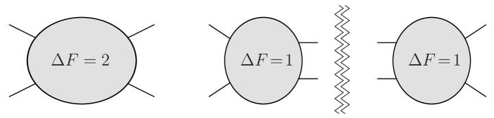
Figure 1: (Left) “family irreducible”: generic $\Delta F=2$ process (Right) “family reducible”: $\Delta F=2$ process can be disconnected into two $\Delta F=1$ parts. There is no horizontal or family charge flowing from the left to the right. The “family reducible” property is a sufficient property for a TeV-scale discrete MFV scenario for any of the groups Eq. (33).

The “family irreducible” property (c.f. Fig. 1) is a sufficient condition for a TeV-scale discrete MFV scenario if the global flavour group $D_{q}$ is built from the following crystal-like groups

$$\Sigma(168)\,,\;\;\Sigma(72\varphi)\,,\;\;\Sigma(216\varphi)\,\;\;\text{and}\;\;\;\Sigma(360\varphi)\;.$$ (33)

Essentially in this case the potentially dangerous invariants factorize ${\cal I}^{(4,4)}\to{\cal I}^{(2,2)}{\cal I}^{(2,2)}$ and the latter have the same invariants as the groups in Eq. (33).

Below we would like to reflect upon this rather general statement via examples and argue that even “family irreducible” type cases may be suitable in (many) perturbative type-models.

• $\Sigma(360\varphi)$ model independent: The most suitable candidate is $\Sigma(360\varphi)$ since the first new invariants appear only at the ${\cal I}^{(4,4)}$ level c.f. Tab 1. The discussion of the previous subsection, c.f. Eq. (32), suggests that the most severe constraints could come from $s\to d$ transitions. We shall attempt at a rough estimate of the real part of $\Delta S=2$ transitions. In the notation of Eq. (12) the effective Lagrangian assumes the following form,

  $$\delta{\cal L}_{\rm eff}^{\Delta S=2}=\frac{\kappa^{4}}{\Lambda^{2}}\sum_{n}c_{n}\,{\cal I}_{n}(\Sigma(360\varphi))^{abc2}_{1stu}\left(\bar{d}\,\Delta_{a}^{\phantom{x}s}\Delta_{b}^{\phantom{x}t}\Delta_{c}^{\phantom{x}u}\,s_{L}\right)\left(\bar{d}\,\Delta_{1}^{\phantom{x}2}\,s_{L}\right)\;,$$ (34)

  where the transition matrices could be either $\Delta_{U}$ or $\Delta_{D}$ (14). The symbol $\kappa$ denotes the Yukawa expansion parameter (2.2). It appears to the fourth power because of the four additional Yukawa matrices. We can now ask the following question: How small does $\kappa$ need to be in order for $C_{\rm dMFV}$ (12) to satisfy the same kind of experimental bounds as for $C_{\rm MFV}$ found in reference [4]? The discussion of the subsection, c.f. Eq. (32), suggests that $s\to d$ could be induced at first order in $\lambda$ as compared to order $|V_{ts}V_{td}^{*}|\sim\lambda^{5}$ in MFV. The total $\Delta S=2$ transition could therefore be ${\cal O}(\lambda^{6})$ as compared to ${\cal O}(\lambda^{10})$ in MFV. According to our reflection above the condition is $\kappa^{4}/\lambda^{4}\simeq 1$ and therefore $\kappa\simeq\lambda\simeq 0.2$.

  

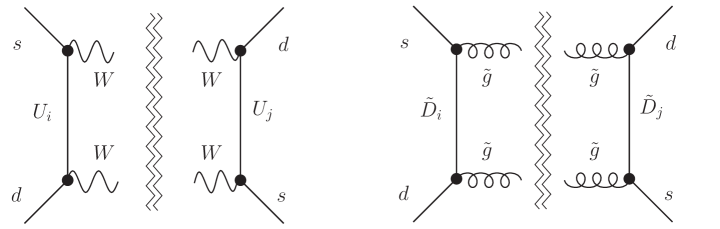
  Figure 2: “family reducible”: The double wiggly lines indicate cuts through the diagrams where there is no (horizontal) family charge flowing. (Left) SM box diagram. (Right) An example of a gluino contribution in the R-parity conserving MSSM.

  

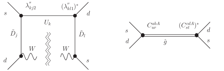
  Figure 3: “family irreducible”: The double wiggle lines indicate cuts through the diagrams where there is no (horizontal) family charge flowing. (Left) An example of a squark contribution in the R-parity violating MSSM e.g. [35]. Yet, this diagram does not generate new flavour structure in discrete MFV. (Right) Engineered example which is family ireducible and does leads to new invariants in dicrete MFV.

• MSSM soft terms and $\Sigma(360\varphi)$: In the MSSM some additional flavour structure enters through the soft terms, e.g. the squark mass matrix $\tilde{m}_{Q}^{2}$, which can be considered to be a ${\cal T}^{(1,1)}$ tensor. It was suggested a long time ago in the spirit of MFV [36] that the nine parameters of the hermitian $\tilde{m}_{Q}^{2}$ could be organized into a Yukawa matrix expansion:

  $$(\tilde{m}_{Q}^{2})_{r}^{\phantom{x}c}=\tilde{m}^{2}\left(a_{1}\delta_{r}^{\phantom{x}c}+b_{1}^{(1)}(\Delta_{U})_{r}^{\phantom{x}c}+b_{1}^{(2)}(\Delta_{D})_{r}^{\phantom{x}c}+b_{2}^{(1)}(\Delta_{U}\Delta_{D}+{\rm h.c.})_{r}^{\phantom{x}c}+....\right)\;.$$

  The first correction of the type given in Eq. (34), in this expansion, would be given by

  $$(\delta\tilde{m}_{Q}^{2})_{r}^{\phantom{x}d}=b_{3}^{(1)}\,{\cal I}_{n}(\Sigma(360\varphi))^{abcd}_{rstu}\,\Delta_{a}^{\phantom{x}s}\Delta_{b}^{\phantom{x}t}\Delta_{c}^{\phantom{x}u}\;.$$ (35)

  Note the assumption of the the Yukawa hierarchy translates into ${\cal O}(b_{1})\simeq{\cal O}(b_{2}\kappa^{-2})\simeq{\cal O}(b_{3}\kappa^{-4})$ for the coefficients .

• family irreducible examples (c.f. Fig 3):
  1. In the R-parity violating MSSM, which is “family irreducible” Fig. 3(left), the fact that each vertex has to be $D_{q}$-invariant prevents the generation of non factorizable ${\cal I}^{(4,4)}$-invariants. This effectively happens because the R-parity violating vertices $\lambda^{{}^{\prime\prime}}_{ijk}U^{i}D^{j}D^{k}$ (U,D are superfields) do not allow for new structures because $\text{\bf 3}\times\text{\bf 3}\times\text{\bf 3}$ contains the trivial representation only once for the groups in Eq. (33).
  2. Lacking a concrete example, let us imagine an effective theory with an interaction vertex ${\cal L}_{\rm eff}\sim C^{abA}_{rs}\,\left(\bar{D}^{r}\Delta_{a}^{\phantom{x}s}D_{b}\right)\,\hat{g}_{A}$. The variable $A$ is an index of a non-trivial representation A appearing in $\bar{\text{\bf 3}}\times\bar{\text{\bf 3}}\times\text{\bf 3}\times\text{\bf 3}=\text{\bf A}+\dots$. The symbol $C^{abA}_{rs}$ denotes a generalized Clebsch-Gordan coefficient that makes the interaction ${\cal D}_{Q_{L}}$ invariant. The scalar particle $\hat{g}$ is supposed to be heavy and, when integrated out, leads to $\Delta S=2$ structure with a (new) non-factorizable ${\cal I}^{(4,4)}$-structure c.f. Fig. 3(right).

6 Epilogue

Before contemplating the scenario we shall briefly summarize our main results. The reduced symmetry leads generally to further invariants and renders the mass-flavour basis transformation matrices observable, which can also be seen as a direct consequence of the absence of the Goldstone bosons themselves. Moreover non-SU(3) invariants do upset MFV hierarchies in a rather anarchic way, c.f. subsection 5.1. In section 4 we have established, through an argument based on the absence of a 27 for discrete SU(3) subgroups, that there necessarily are new invariants for ${\cal I}^{(4,4)}$. The latter enter generic $\Delta F=2$ transitions (16). In cases where the $\Delta F=2$ process is generated via two $\Delta F=1$ subprocesses, which we called “family reducible”, the invariant factorizes: ${\cal I}^{(4,4)}\to{\cal I}^{(2,2)}{\cal I}^{(2,2)}$. For the latter the groups $\Sigma(168)$, $\Sigma(72\varphi)$, $\Sigma(216\varphi)$ and $\Sigma(360\varphi)$ do provide enough symmetry to immitate SU(3) at this level and thus are valid candidates for a TeV-scale discrete MFV scenario with Yukawa expansion parameters of the order of $\kappa_{\Sigma(360\varphi)}\simeq 0.2$. Models which are not of the “family reducible”-type may still be viable candidates; especially if they are perturbative. An overview of the number of invariants is given in Tab. 1. Below we shall add a few not necessarily connected thoughts on MFV and the framework proposed here.

• Origin of discrete symmetry: One might of course ask the question about the origin of such discrete symmetries. They might originate from compactifications in String Theory, where it was found that the trihedral group $\Delta(54)$ can appear [39] or they could appear from the breaking of a continuous symmetry, c.f. [40] for a recent investigation. The latter has to happen, presumably, at some high energy in order not to make the so far unseen familons too visible. We would like to add that whether global symmetries originate from local ones or not can have subtle physical consequences [41].

• This and that: Surely it is possible that the groups ${\cal D}$ (2.2) are of different types. We have focused on ${\cal D}_{Q_{L}}$, which gouverns the $D(U)_{L}\to D(U)_{L}^{\prime}$ transitions. The groups ${\cal D}_{D_{R}}$ would matter once we consider $D_{R}\to D_{R(L)}^{\prime}$ type operators, where again the groups (33) would provide most protection. Needless to say that if the question of flavour is not linked to a scale close to the TeV-scale, and the breaking of $D_{q}$ (or $G_{q}$) happens at high scale, then experimental bounds do not favour any particular groups. Though in the MSSM for example the implementation of MFV is related to supersymmetry breaking through the soft terms [36, 4] (• ‣ 5.2) and this in turn suggests a link of flavour to the hierarchy problem.

• Embeddings: The formulation (2.2) could be refined by constructing a discrete subgroups of $G_{q}$ (3) which does not factor into direct products of SU(3) subgroups. Much in the same way as the discrete subgroup $\Sigma(81)\subset U(3)\thickapprox U(1)\times SU(3)\,$ cannot be written as a direct product of a discrete SU(3) and U(1) subgroup; $\Sigma(81)\notin{\cal D}_{U(1)}\times{\cal D}_{SU(3)}$. One might wonder what the consequences for the invariants are.

• Model of (d)MFV: MFV is an empirically motivated effective field theory approach. Up to now no explicit model of MFV has been constructed. Though the seeds of a scenario were put forward in [15, 7]. As hinted at in the introduction the relation between the MFV scale $\sqrt{16\pi^{2}C_{\rm MFV}}$ and the breaking scale(s) $f_{F}$ can only be answered model by model. It has to be added that a model of MFV without the input of the CKM and mass structure seems to be at the same level of difficulty as constructing a theory of flavour which has proven to be a hard problem. One should not forget that besides being predictive and testable MFV has other appealing properties: In an R-parity violating MSSM, MFV provides enough protection to evade bounds on the proton decay [37]. MFV also serves as a reference point for any model with flavour structure and facilitates comparison of different models.

Our aim, in this work, was to point out general issues of implementing MFV via a discrete group. We would hope that this work would be of some help for further investigations towards more specific models, where for one reason or another one or the other invariant does not turn out to be as menacing as in the essentially model independent approach followed here.

Appendix A Examples of invariants in the flavour basis

In this appendix we discuss characteristic invariants of specific groups (in the flavour basis). From section 4.1 we already know that new invariants are present at the level of the effective theory. The aim of this appendix is to present a few instructive (concrete) examples. We shall use the notation (15) for the left handed $D$-quarks.

A.1 Crystal groups $\Sigma$

We shall discuss $\Sigma(60)$ and $\Sigma(168)$ which are both instructive.

The group $\Sigma(60)$

The representations of $\Sigma(60)\thickapprox A_{5}\thickapprox I_{\rm cosahedral}\subset SO(3)$ have for instance been studied in [44]. There are two real 3D irreps which we shall denote by $\text{\bf 3}_{1}$ and $\text{\bf 3}_{2}$. Their product representation takes the following form

$$\text{\bf 3}_{i}\times\text{\bf 3}_{i}=\text{\bf 1}+\text{\bf 3}_{i}+\text{\bf 5}\;,\qquad i=1..2\;.$$ (A.1)

The $\text{\bf 3}_{i}$ on the right hand side (RHS) of (A.1), with (15) , reads

$$\text{\bf 3}_{i}\sim(\bar{D}_{3}D_{2}-\bar{D}_{2}D_{3},\bar{D}_{1}D_{3}-\bar{D}_{3}D_{1},\bar{D}_{2}D_{1}-\bar{D}_{1}D_{2})^{T}\;.$$ (A.2)

Since $\bar{\text{\bf 3}}_{i}=\text{\bf 3}_{i}$ the singlet is obtained by simply taking the scalar product of the vector above

$${\cal I}^{(2,2)}_{\Sigma(60)_{2}}=\bar{D}_{3}D_{2}\bar{D}_{3}D_{2}+\dots\;.$$ (A.3)

The group $\Sigma(60)$ does allow for a $\Delta F=2$ structure even in the absence of any Yukawa matrices. The symmetry is simply not strong enough to constrain flavour transitions in any way.

The group $\Sigma(168)$

The isomorphisms of this group are: $\Sigma(168)\thickapprox{\rm PSL}(2,\mathbb{F}_{7})\thickapprox{\rm GL}(3,\mathbb{F}_{2})$ [24]. The irreps can be read off from (23) and since the first non-trivial representations have the same dimension this implies that they are identical [24], $\bar{\text{\bf 3}}\times\text{\bf 3}=\text{\bf 1}+\text{\bf 8}$. The 8 is therefore real but the difference appears at the level of product of two 8 c.f. Eq. (4.2). As a consequence of the general discussion in subsection 4.1 the absence of a 27 implies further invariants. We may construct one of these invariants with the results given in [24] as follows: Consider the product $\text{\bf 3}\times\text{\bf 3}=\bar{\text{\bf 3}}+\text{\bf 6}$ and the information that the 6D is real, i.e. $\bar{\text{\bf 6}}=\text{\bf 6}$, we may infer that the following product $\text{\bf 3}\times\text{\bf 3}\times\text{\bf 3}\times\text{\bf 3}=1\!\cdot\!\text{\bf 1}+...$ contains the trivial representation once. The invariant tensor may be read off from [24]

$$d_{abcd}=d^{abcd}=\sum_{\alpha\beta}K_{ab}^{\alpha}K_{cd}^{\beta}C_{\alpha\beta}\;=\;\left\{\begin{array}[]{ll}1/\sqrt{2}&\quad abcd=\{1113,2221,3332\}\;\;\&\text{ cyclic}\\ 0&\quad\text{otherwise}\end{array}\right.\;,$$ (A.4)

where cyclic refers to $1113\to 3111\to 1311\to 1131$ etc. The first equality sign above is to be understood on the level of indices and not at the level of tensors. Note that the invariant

$$f=d^{abcd}D_{a}D_{b}D_{c}D_{d}\sim D_{3}(D_{1})^{3}+D_{1}(D_{2})^{3}+D_{2}(D_{3})^{3}\;,$$ (A.5)

just corresponds to Klein’s famous quartic invariant [45]. From (A.4) we can build an invariant of the form

$$({\cal I}_{\Sigma(168)_{3}})^{abcd}_{rstu}=d^{abcd}d_{rstu}\;.$$ (A.6)

This invariant tensor, with field content (16), leads to terms of the form

$${\cal I}^{(4,4)}_{\Sigma(168)_{3}}\sim\bar{D}_{1}\bar{D}_{1}\Delta_{1}^{\phantom{x}1}\Delta_{2}^{\phantom{x}3}D_{2}D_{2}+\text{permutations}\;.$$ (A.7)

Revealing a rather anarchic structure of flavour transitions even in the flavour basis. Moreover the seventh tensor ${\cal I}^{(3,3)}_{\Sigma(168)_{7}}$, c.f. Tab. 1 can easily be constructed

$$({\cal I}^{(3,3)}_{\Sigma(168)_{7}})^{abc}_{rst}=d_{abci}d^{irst}\;.$$ (A.8)

At last we would like to remark that the tensor $d_{ab}^{\phantom{xy}cd}=d_{abij}d^{ijcd}$

$$d_{ab}^{\phantom{xy}cd}\;=\;\left\{\begin{array}[]{ll}1&\quad a=b=c=d\\ 1/2&\quad a=c,b=d\;\text{ or }\;a=d,b=c\\ 0&\quad\text{otherwise}\end{array}\right.\;,$$ (A.9)

acts, as expected, like a Kronecker symbol in the 6-space.

A.2 The trihedral groups $\Delta(3n^{2})$ and $\Delta(6n^{2})$

The main purpose of this subsection is to give some explicit non-SU(3) ${\cal I}^{(2,2)}$ invariants. In passing we would like to mention that as long as no real representations are generated, we have checked that for specific $n,k,l$ this is the case, all flavour transitions are gouverned by the Yukawa matrices in the flavour basis. This fact is interesting but irrelevant to our work because the passage to the mass basis changes everything c.f. subsection 5.1. At last we argue that the $D$-groups are subgroups of an appropriate $\Delta(6g^{2})$ which is not known to the authors from any other source.

The groups $\Delta(3n^{2})$

The group admits the following isomorphism [23] $\Delta(3n^{2})\thickapprox(\mathbb{Z}_{n}\times\mathbb{Z}_{n})\rtimes\mathbb{Z}_{3}$. As previously mentioned this group has only one and 3D irreps. They are labeled by the pair $(k,l)$ where $k,l=0..n-1$ but $(k,l)\neq(0,0)$ (and additionally $(k,l)\neq s(n/3,n/3)$ with $s=1..2$ for $n=3\mathbb{Z}$) and the following pairs, $(k,l)\thickapprox(-k-l,,k)\thickapprox(l,-k-l)$, describe equivalent irreps. The complex conjugate representation is obtained by reversing the sign of $k,l$, i.e. $\bar{\text{\bf 3}}_{(k,l)}=\text{\bf 3}_{(-k,-l)}$. Anything relevant to us can be gained from the following Kronecker product [23, 25]

$$\bar{\text{\bf 3}}_{(k,l)}\times\text{\bf 3}_{(k,l)}=\text{\bf 3}_{(0,0)}+\text{\bf 3}_{(-2k-l,k-l)}+\text{\bf 3}_{(2k+l,l-k)}\;,$$ (A.10)

and the branching rules for the RHS of (A.10) are

$$\text{\bf 3}_{(0,0)} \to\text{\bf 1}_{0,0}+\text{\bf 1}_{1,0}+\text{\bf 1}_{2,0}\;,\qquad$$ (A.11)

and for $n=3\mathbb{Z}$ with $k,l\in\mathbb{Z}n/3$, which reduces to $(k,l)=(0,\pm n/3)$ under equivalences,

$$\text{\bf 3}_{(\frac{n}{3},\frac{n}{3})}+\text{\bf 3}_{(-\frac{n}{3},-\frac{n}{3})} \to\text{\bf 1}_{0,1}+\text{\bf 1}_{1,1}+\text{\bf 1}_{2,1}+\text{\bf 1}_{0,2}+\text{\bf 1}_{1,2}+\text{\bf 1}_{2,2}\;,$$ (A.12)

there are nine one dimensional irreps. With (15) and for $(k,l)=(0,n/3)$ they take on the form

$$\text{\bf 1}_{r,0} \sim \bar{D}^{1}D_{1}+\omega^{-r}\bar{D}^{2}D_{2}+\omega^{r}\bar{D}^{3}D_{3}\;,$$

$$\text{\bf 1}_{r,1} \sim \bar{D}^{2}D_{1}+\omega^{-r}\bar{D}^{3}D_{2}+\omega^{r}\bar{D}^{1}D_{3}\;,$$

$$\text{\bf 1}_{r,2} \sim \bar{D}^{3}D_{1}+\omega^{-r}\bar{D}^{1}D_{2}+\omega^{r}\bar{D}^{2}D_{3}\;,$$ (A.13)

and for $(k,l)=(0,-n/3)$ the roles of $\text{\bf 1}_{r,1/2}$ are reversed [25]. Two of the generators, $a$ and $c$, act in a non-trivial manner [25]: $a\circ\text{\bf 1}_{r,s}=\omega^{r}\text{\bf 1}_{r,s}\;,c\circ\text{\bf 1}_{r,s}=\omega^{s}\text{\bf 1}_{r,s}$ implying $\text{\bf 1}_{r,s}\times\text{\bf 1}_{r^{\prime},s^{\prime}}=\text{\bf 1}_{r+r^{\prime},s+s^{\prime}}$. Note $\text{\bf 1}_{0,0}$ is therefore the only singlet. For any $n$ and $k,l$ there are at least five invariant tensor at the level of ${\cal I}^{(2,2)}$, as compared to two for SU(3) c.f. Tab. 1. For the symmetric contraction $\bar{D}^{a}\bar{D}^{b}D_{c}D_{d}$ the $\text{\bf 1}_{1,0}\times\text{\bf 1}_{2,0}$ invariant reads

$${\cal I}^{(2,2)}_{\Delta(3n^{2})_{2}} = \;{\cal I}^{(2,2)}_{\Delta(3n^{2})_{1}}-3(\bar{D}^{1}D_{1}\bar{D}^{2}D_{2}+\bar{D}^{2}D_{2}\bar{D}^{3}D_{3}+\bar{D}^{1}D_{1}\bar{D}^{3}D_{3})\;,$$

$${\cal I}^{(2,2)}_{\Delta(3n^{2})_{1}} = \;(\bar{D}^{1}D_{1}+\bar{D}^{2}D_{2}+\bar{D}^{3}D_{3})^{2}\;,$$ (A.14)

where we have indicated the SU(3) invariant ${\cal I}_{1}$ for notational convenience. For the sake of completeness we shall indicate the explicit 3D irreps, which can be obtained from appendix D of reference [25], up to a single transformation of the generator $a$,

$$\text{\bf 3}_{(-2k-l,k-l)}\sim(\bar{D}_{1}D_{2},\bar{D}_{2}D_{3},\bar{D}_{3}D_{1})^{T}\;,\quad\bar{\text{\bf 3}}_{(-2k-l,k-l)}\sim(\text{\bf 3}_{(2k+l,l-k)})^{*}\;.$$ (A.15)

From the explicit forms (A.2) and (A.15) it is a simple matter to obtain the ${\cal I}^{(2,2)}$ invariants and even beyond. To this end we shall briefly discuss two cases of $\Delta(3n^{2})$ which are popular in the literature.

• $n=2:\Delta(12)\thickapprox A_{4}$. In fact this group was brought into particle physics as early as 1979 [46]. There is only one 3D irrep with $(k,l)=(0,1)$, which is real. The latter fact can either be checked explicitly, asserted from there being only one 3D irrep or inferred from the fact that $A_{4}\subset SO(3)$. The number of ${\cal I}^{(2,2)}$ invariants is seven and the reality of the 3 allows to form an invariant

  $${\cal I}^{(2,2)}_{\Delta(3n^{2})_{4}}=(\bar{D}_{1}D_{2})^{2}+(\bar{D}_{2}D_{3})^{2}+(\bar{D}_{3}D_{1})^{2}\;,\text{and}\quad{\cal I}_{5}={\cal I}_{4}^{*}.$$ (A.16)

• $n=3:\Delta(27)$ is the first group that admits nine one-dimensional irreps. The remaining ones completing the relation (11) is a complex conjugate pair of 3D irreps. There are nine ${\cal I}^{(2,2)}$ invariants, which can easily be obtained from (A.2).

The groups $\Delta(6n^{2})$

The group admits the following isomorphism [23] $\Delta(6n^{2})\thickapprox(\mathbb{Z}_{n}\times\mathbb{Z}_{n})\rtimes S_{3}\;.$ The irreps are 6, 3, 2 and 1D. The 6D representations $\text{\bf 6}_{(k,l)}$ are labeled by a pair $(k,l)$, where $k=0..(n\!-\!1)$ and neither $k=0$, $l=0$ nor $k+l=0\mod n$ (and additionally $(k,l)\neq s(n/3,n/3)$ with $s=1..2$ for $n=3\mathbb{Z}$). Moreover the following six pairs $(k,l)\thickapprox(-k-l,k)\thickapprox(l,-k-l)\thickapprox(-l,-k)\thickapprox(k+l,-l)\thickapprox(-k,k+l)$, describe equivalent irreps. There are two types of 3D irreps originating from $\text{\bf 6}_{k,l}$ when $k+l=0\mod n$ and $(k,l)\neq(0,0)$. The two types of representations can therefore be labeled by ${\text{\bf 3}}_{\text{\bf 1}}^{(l)}$ and ${\text{\bf 3}}_{\text{\bf 2}}^{(l)}$. Complex conjugate irreps are obtained by reversing the sign of $(k,l)$ and $(l)$ respectively. For $n\in 3\mathbf{Z}$ there are three further 2D irreps denoted by ${\text{\bf 2}}_{\text{\bf 2}},{\text{\bf 2}}_{\text{\bf 3}},{\text{\bf 2}}_{\text{\bf 4}}$ [26], which are not relevant for ${\cal I}^{(2,2)}$ invariants. The Kronecker product for the latter reads [26]:

$$(\bar{{\text{\bf 3}}}_{\text{\bf 1}}^{(l)}\times{\text{\bf 3}}_{\text{\bf 1}}^{(l)})\times(\bar{{\text{\bf 3}}}_{\text{\bf 1}}^{(l)}\times{\text{\bf 3}}_{\text{\bf 1}}^{(l)})=({\text{\bf 3}}_{\text{\bf 1}}^{(0)}+\text{\bf 6}_{(l,l)})\times({\text{\bf 3}}_{\text{\bf 1}}^{(0)}+\text{\bf 6}_{(l,l)})\;,$$ (A.17)

where the explicit vectors on the RHS, using the parametrization (15), are

$${\text{\bf 3}}_{\text{\bf 1}}^{(0)}=(\bar{D}^{1}D_{1},\bar{D}^{2}D_{2},\bar{D}^{3}D_{3})^{T}\;,\quad\text{\bf 6}_{(l,l)}=(\bar{D}^{1}D_{3},\bar{D}^{3}D_{2},\bar{D}^{2}D_{1},\bar{D}^{1}D_{2},\bar{D}^{2}D_{3},\bar{D}^{3}D_{1})^{T}\;.$$

Our form looks slightly more symmetric than the one in reference [26] because we have chosen the $(l,l)$ rather than the $(-l,2l)$ representative. The remaining relevant Kronecker products are:

$${\text{\bf 3}}_{\text{\bf 1}}^{(0)}\times{\text{\bf 3}}_{\text{\bf 1}}^{(0)} = \;{\text{\bf 3}}_{\text{\bf 1}}^{(0)}+\text{\bf 6}_{(0,0)}\;,$$

$${\text{\bf 3}}_{\text{\bf 1}}^{(0)}\times\text{\bf 6}_{(l,l)} = \;3\cdot\text{\bf 6}_{(l,l)}\;,$$

$$\text{\bf 6}_{(l,l)}\times\text{\bf 6}_{(l,l)} = \;\text{\bf 6}_{(0,0)}+\text{\bf 6}_{(2l,2l)}+\text{\bf 6}_{(3l,0)}+\text{\bf 6}_{(0,3l)}+\text{\bf 6}_{(-l,2l)}+\text{\bf 6}_{(2l,-l)}\;.$$ (A.18)

The RHS remains the same when ${\text{\bf 3}}_{\text{\bf 1}}$ is exchanged with ${\text{\bf 3}}_{\text{\bf 2}}$ on the left hand side [26]. The relevant branching rules are:

$${\text{\bf 3}}_{\text{\bf 1}}^{(0)}\to\text{\bf 1}_{1}+\text{\bf 2}_{1}\;,\quad\text{\bf 6}_{(0,0)}\to\text{\bf 1}_{1}+\text{\bf 2}_{1}+\text{\bf 1}_{2}+\text{\bf 2}_{2}\;.$$ (A.19)

The Clebsch-Gordan coefficient of ${\text{\bf 3}}_{\text{\bf 1}}^{(0)}$ and $\text{\bf 6}_{(0,0)}$ on the RHS of the top equation (A.2) are immediate from the ones of (A.17) and the ones for $\text{\bf 6}_{(0,0)}$ are [26]

$$\text{\bf 6}_{(0,0)}\sim(\bar{D}^{1}D_{6},\bar{D}^{2}D_{5},\bar{D}^{3}D_{4},\bar{D}^{4}D_{3},\bar{D}^{5}D_{2},\bar{D}^{6}D_{1})\;.$$

We have used an obvious generalization of (15). It can be said that at the ${\cal I}^{(2,2)}$ level there are at least three invariants to be compared to two for SU(3) c.f. Tab. 1. The Clebsch-Gordan coefficients allow us to obtain them explicitly. We leave it to the reader to figure out the precise association of $(n,l)$ and the number of invariants. The question is then how the singlets in Eq. (A.2) can be obtained from ${\text{\bf 3}}_{\text{\bf 1}}^{(0)}$ and $\text{\bf 6}_{(0,0)}$. In both cases the generators $c$ and $d$ act trivially and then it remains to work out which combination remains invariant under the two remaining generators $a$ and $b$. Not surprisingly they are obtained by summing all the entries of the vectors. The correspondences are

$${\text{\bf 3}}_{\text{\bf 1}}^{(0)}\;\;\leftrightarrow\;\; {\cal I}^{(2,2)}_{\Delta(6n^{2})_{1}}=\bar{D}^{1}D_{1}\bar{D}^{1}D_{1}+\bar{D}^{2}D_{2}\bar{D}^{2}D_{2}+\bar{D}^{3}D_{3}\bar{D}^{3}D_{3}\;,$$

$$\text{\bf 6}_{(0,0)}\;\;\leftrightarrow\;\; {\cal I}^{(2,2)}_{\Delta(6n^{2})_{2}}=\bar{D}^{1}D_{2}\bar{D}^{2}D_{1}+\bar{D}^{1}D_{3}\bar{D}^{3}D_{1}+\bar{D}^{3}D_{2}\bar{D}^{2}D_{3}\;.$$ (A.20)

It worth noting that both $\text{\bf 6}_{(0,0)}$ give rise to the same invariant ${\cal I}^{(2,2)}_{2}$ under the symmetric contraction $\bar{D}^{a}\bar{D}^{b}D_{c}D_{d}$. Note that ${\cal I}_{\Delta(6n^{2})_{1,2}}$ are different from ${\cal I}_{\Delta(3n^{2})_{1,2}}$ but since the two pairs are linearly dependent they are effectively the same.

A.2.1 The $(D)$-groups are subgroups of $\Delta(6n^{2})$

In the classic work of Miller et al [16] the so-called $(C)$ and $(D)$-subgroups of SU(3) are defined as matrix groups. In [28] it is shown that the $(C)$-groups are nothing but a special case of $\Delta(3n^{2})$. We shall argue here that the $(D)$-groups are nothing but subgroups of an appropriate $\Delta(6g^{2})$.

In [28], the generators of the $(D)$-groups have been worked out,

$$H=\left(\begin{matrix}\eta^{a}&0&0\\ 0&\eta^{b}&0\\ 0&0&\eta^{-a-b}\end{matrix}\right),\quad T=\left(\begin{matrix}0&1&0\\ 0&0&1\\ 1&0&0\end{matrix}\right),\quad R=\left(\begin{matrix}\delta^{r}&0&0\\ 0&0&\delta^{s}\\ 0&-\delta^{-r-s}&0\end{matrix}\right),$$ (A.21)

where $\eta\equiv\exp(2\pi i/n)$, $\delta\equiv\exp(2\pi i/d)$. They give rise to a collection of (not necessarily simple) six-parameter subgroups $D(n,a,b;d,r,s)$ of $SU(3)$. When viewed as a matrix subgroup of $SU(3)$ in its fundamental 3 representation, the matrices belonging to these $(D)$-groups have exactly one non-zero entry in every row and column. Furthermore, the non-zero entries are powers of the g-th root of unity, with $g={\rm lcm}(n,d,2)$, where ${\rm lcm}$ stands for the lowest common multiple. The collection of all such matrices evidently forms a group with $6\times g^{2}$ elements (the non-zero entries in the first and second row determine the non-zero entry in the third, and there are six ways to place the elements). As this group must be just the $\Delta(6n^{2})$ group with $n=g$, these $(D)$-groups are subgroups (proper or not) of the $\Delta(6n^{2})$ groups. As such, they cannot possess an irreducible representation whose dimension exceeds six. An immediate consequence is that the group $D(n,a,b;d,r,s)$ shares the two invariants Eq. (A.2) with $\Delta(6g^{2})$. The latter assertion can also be checked explicitly from the generators given in (A.21).

We would like to add that it was shown in [29] that whereas the $(C)$-groups can be interpreted as irreducible representations of $\Delta(3g^{2})$, this is not (always) the case for $(D)$-groups with respect to $\Delta(6g^{2})$.

Appendix B Embedding of discrete groups into SU(3)

We would like to settle the question of whether it possible to approximate an arbitrary SU(3) element (a basis transformation) by an element of a discrete group ${\cal D}\subset$ SU(3) suitably embedded into SU(3). The embedding of ${\cal D}$ into SU(3) ca be varied by conjugation with an arbitrary SU(3) matrix. The problem therefore reduces to the question of whether there exist a $D\in{\cal D}$ and $B\in SU(3)$ for a specific $A\in SU(3)$ such that

$$A\simeq BDB^{\dagger}\;.$$ (A.22)

We shall argue below that for $\Delta(3n^{2})$ this is possible. Eq. (A.22) is true if $A$ and $D$ have (approximately) the same invariants. The invariants are given by the coefficients of the characteristic polynomial which are just the trace of the matrix and the trace of the square of the matrix. A sufficient condition for the traces to be (approximately) the same is that the eigenvalues are (approximately) the same. This immediately eliminates the crystal groups since there traces, i.e. characters, only assume very specific values. This can be inferred from the character tables. We shall proceed our argument via the eigenvalues. An SU(3) matrix has in general three eigenvalues of the form $\lambda_{i}=e^{i\phi_{i}}$ with the determinant condition $\phi_{1}+\phi_{2}+\phi_{3}=0\mod 2\pi$. The generators of $\Delta(3n^{2})$ in the representation $\text{\bf 3}_{(k,l)}$ read [25]

$$a=\begin{pmatrix}0&1&0\\ 0&0&1\\ 1&0&0\end{pmatrix},~{}~{}~{}~{}c=\begin{pmatrix}\eta^{l}&0&0\\ 0&\eta^{k}&0\\ 0&0&\eta^{-k-l}\end{pmatrix},~{}~{}~{}~{}d=\begin{pmatrix}\eta^{-k-l}&0&0\\ 0&\eta^{l}&0\\ 0&0&\eta^{k}\end{pmatrix}\ \,,$$ (A.23)

with $\eta=\exp(2\pi i/n)$ and it is readily seen that the parameters $k,l,n$ can be adjusted such that the eigenvalues, of for example $c$, are arbitrarily close to any pair of unitary complex numbers. The third one is fixed in both cases by the determinant condition. For $\Delta(6n^{2})$ this is also possible: The elements $c_{3_{1}}^{a}d_{3_{1}}^{b}$, with generators $c_{3_{1}},d_{3_{1}}$ as given in [26], approximate any two eigenvalues with arbitrary precision for suitable $a,b,n,l\in\mathbb{Z}$.

We conclude that $\Delta(3n^{2})$ and $\Delta(6n^{2})$ contrary to the crystal groups can be embedded into SU(3) such that one of its elements is arbitrarily close to any SU(3) element.

References

- [1] R. S. Chivukula and H. Georgi, Phys. Lett. B 188 (1987) 99.
- [2] G. ’t Hooft, Phys. Rev. Lett. 37 (1976) 8.
- [3] S. Dimopoulos, H. Georgi and S. Raby, Phys. Lett. B 127 (1983) 101.
- [4] G. D’Ambrosio, G. F. Giudice, G. Isidori and A. Strumia, Nucl. Phys. B 645 (2002) 155 [arXiv:hep-ph/0207036].
- [5] M. Bona et al. [UTfit Collaboration], JHEP 0803 (2008) 049 [arXiv:0707.0636 [hep-ph]].
- [6] V. Cirigliano, B. Grinstein, G. Isidori and M. B. Wise, Nucl. Phys. B 728 (2005) 121 [arXiv:hep-ph/0507001]. S. Davidson and F. Palorini, Phys. Lett. B 642 (2006) 72 [arXiv:hep-ph/0607329].
- [7] T. Feldmann, M. Jung and T. Mannel, Phys. Rev. D 80 (2009) 033003 [arXiv:0906.1523 [hep-ph]].
- [8] F. Wilczek, Phys. Rev. Lett. 49 (1982) 1549. D. B. Reiss, Phys. Lett. B 115 (1982) 217.
- [9] A. Manohar and H. Georgi, Nucl. Phys. B 234 (1984) 189.
- [10] J. L. Feng, T. Moroi, H. Murayama and E. Schnapka, Phys. Rev. D 57 (1998) 5875.
- [11] M. Albrecht, T. Feldman and T. Mannel in preparation
- [12] S. Weinberg, “The quantum theory of fields. Vol. 2: Modern applications,” Cambridge, UK: Univ. Pr. (1996) 489 p
- [13] F. Wilczek and A. Zee, Phys. Rev. Lett. 42 (1979) 421.
- [14] A. L. Kagan, G. Perez, T. Volansky and J. Zupan, arXiv:0903.1794 [hep-ph].
- [15] T. Feldmann and T. Mannel, Phys. Rev. Lett. 100 (2008) 171601
- [16] Chapter XII in G. A. Miller, H. F. Blichfeldt, and L. E. Dickson, Theory and Applications of Finite Groups, John Wiley & Sons, New York 1916, and Dover Edition 1961;
- [17] W. M. Fairbairn, T. Fulton, and W. H. Klink, J. Math. Phys. 5:1038, 1964.
- [18] A. J. Buras, P. Gambino, M. Gorbahn, S. Jager and L. Silvestrini, Phys. Lett. B 500 (2001) 161 [arXiv:hep-ph/0007085].
- [19] G. Altarelli, arXiv:0905.3265 [hep-ph].
- [20] G. Isidori, F. Mescia, P. Paradisi, C. Smith and S. Trine, JHEP 0608 (2006) 064
- [21] H. Georgi, Phys. Rev. Lett. 98 (2007) 221601 [arXiv:hep-ph/0703260].
- [22] A. Bovier and D. Wyler, J. Math. Phys. 22 (1981) 2108.
- [23] A. Bovier, M. Luling and D. Wyler, J. Math. Phys. 22 (1981) 1543.
- [24] C. Luhn, S. Nasri and P. Ramond, J. Math. Phys. 48 (2007) 123519 [arXiv:0709.1447 [hep-th]].
- [25] C. Luhn, S. Nasri and P. Ramond, J. Math. Phys. 48 (2007) 073501 [arXiv:hep-th/0701188].
- [26] J. A. Escobar and C. Luhn, J. Math. Phys. 50 (2009) 013524 [arXiv:0809.0639 [hep-th]].
- [27] W. M. Fairbairn and T. Fulton, J. Math. Phys. 23 (1982) 1747.
- [28] P. O. Ludl, arXiv:0907.5587 [hep-ph].
- [29] P. O. Ludl, arXiv:1101.2308 [math-ph].
- [30] H. Georgi, Front. Phys. 54 (1982) 1.
- [31] R. Slansky, Phys. Rept. 79 (1981) 1.
- [32] P. E. Desmier, R. T. Sharp and J. Patera, J. Math. Phys. 23 (1982) 1393.
- [33] S. Weinberg, “The Quantum theory of fields. Vol. 1: Foundations,” Cambridge, UK: Univ. Pr. (1995) 609 p
- [34] L. Wolfenstein, Phys. Rev. Lett. 13 (1964) 562.
- [35] M. Misiak, S. Pokorski and J. Rosiek, Adv. Ser. Direct. High Energy Phys. 15 (1998) 795 [arXiv:hep-ph/9703442].
- [36] L. J. Hall and L. Randall, Phys. Rev. Lett. 65 (1990) 2939.
- [37] E. Nikolidakis and C. Smith, Phys. Rev. D 77 (2008) 015021 [arXiv:0710.3129 [hep-ph]].
- [38] L. Mercolli and C. Smith, Nucl. Phys. B 817 (2009) 1 [arXiv:0902.1949 [hep-ph]].
- [39] T. Kobayashi, H. P. Nilles, F. Ploger, S. Raby and M. Ratz, Nucl. Phys. B 768 (2007) 135 [arXiv:hep-ph/0611020].
- [40] A. Adulpravitchai, A. Blum and M. Lindner, arXiv:0907.2332 [hep-ph].
- [41] L. M. Krauss and F. Wilczek, Phys. Rev. Lett. 62 (1989) 1221.
- [42] E. Ma, Phys. Lett. B 649 (2007) 287 [arXiv:hep-ph/0612022].
- [43] C. Hagedorn, M. A. Schmidt and A. Y. Smirnov, Phys. Rev. D 79 (2009) 036002 [arXiv:0811.2955 [hep-ph]].
- [44] L. L. Everett and A. J. Stuart, arXiv:0812.1057 [hep-ph].
- [45] Felix Klein ”Ueber die Transformationen siebenter Ordnung der elliptischen Funktionen” Math. Ann. vol. 14, 1879. p 428-471
- [46] D. Wyler, Phys. Rev. D 19 (1979) 3369.