Non-Markovian control of qubit thermodynamics by frequent quantum measurements

Abstract

We explore the effects of frequent, impulsive quantum nondemolition measurements of the energy of two-level systems (TLS), alias qubits, in contact with a thermal bath. The resulting entropy and temperature of both the system and the bath are found to be completely determined by the measurement rate, and unrelated to what is expected by standard thermodynamical rules that hold for Markovian baths. These anomalies allow for very fast control of heating, cooling and state-purification (entropy reduction) of qubits, much sooner than their thermal equilibration time.

I Introduction

Non-Markovian quantum thermodynamics of two level systems (TLS) in contact with a bath has surprising aspects in store. According to standard Markov thermodynamics, the TLS (alias qubit) thermal equilibration process is expected to progress monotonically, accompanied by increase of the entropy, at least on average landau1980spe ; spo78 ; ali79 ; jar97 ; lin74 . Yet drastic deviations from this trend are revealed when considering impulsive disturbances of thermal equilibrium between TLS and a bath schulman2006rue ; piilo2007qbm . These effects bear certain similarities to the work described in Nieu02 . We have shown ere08Nature that frequent and brief quantum non demolition (QND) measurements of the TLS energy-states entail unfamiliar anomalies of the entropy and temperature of both system and bath, which become unrelated to what is known from standard, Markovian thermodynamic rulesspo78 ; lin74 : (i) a transition from heating to cooling of the TLS ensemble as we vary the interval between consecutive measurements on the time scale of the inverse energy separation of the qubit levels; and (ii) correspondingly, oscillations of the entropy relative to that of the equilibrium state.

Here we present an in-depth study of short-time evolution of quantum systems coupled to a bath, interrupted by frequent measurements. We first discuss in Sec. II the initial equilibrium state relevant to our scenario. Sec. III then describes the measurement-induced disturbance of equilibrium. In Sec. IV we present a master equation analysis of the post-measurement evolution and a discussion of the heating and cooling requirements. Cooling conditions and entropy evolution of the system are discussed in Sec. V and  VI, respectively. A discussion of possible experimental realizations is given in Sec. VII.

II System-bath entanglement at equilibrium

II.1 Hamiltonian

The following Hamiltonian describes the qubit system that interacts with the bath.

$$H_{tot}=H_{S}+H_{B}+H_{SB}.$$ (1)

Here $H_{tot}$ pertains to the coupled system and bath and consists of:

$$H_{S}= \hbar\omega_{a}{|e\rangle}{\langle e|},$$ (2)

$$H_{B}= \hbar\sum_{\lambda}\omega_{\lambda}a_{\lambda}^{\dagger}a_{\lambda},$$ (3)

$$H_{SB}= \mathcal{SB},\mathcal{S}=\sigma_{x},~{}~{}\mathcal{B}=\hbar\sum_{\lambda}\left(\kappa_{\lambda}a_{\lambda}+\kappa_{\lambda}^{*}a_{\lambda}^{\dagger}\right),$$ (4)

where $\mathcal{S}$ and $\mathcal{B}$ are the system and bath operators, respectively, in the system-bath interaction $H_{SB}$, $a_{\lambda}(a^{\dagger}_{\lambda})$ are the annihilation (creation) operators, and $\kappa_{\lambda}$ is the matrix element of the weak coupling to bath mode $\lambda$. We stress that in the interaction Hamiltonian ($H_{SB}$) we do not invoke the rotating-wave approximation (RWA)coh92 , namely, we do not impose energy conservation between the system and the bath, on the time scales consideredkof04 .

II.2 Qubit state mixedness at equilibrium

At equilibrium, the qubit and the bath are in an entangled state. To find the mean energy mixedness (impurity) of the qubit (TLS) at a given temperature $T$, one needs the equilibrium density matrix for the total system $\rho_{Eq}=\exp(-\beta H_{tot})/Z$, where $Z$ is the partition function and $1/\beta=k_{B}T$.

Using Heims perturbation theory Heims one can expand $\rho_{Eq}$ as

$$\rho_{Eq}=\frac{1}{Z}{\rm e}^{-\beta(H_{0}+H_{SB})}\\ =\frac{1}{Z}{\rm e}^{-\beta H_{0}}[1+\epsilon S_{1}+\epsilon^{2}S_{2}+O(\epsilon^{3})+\cdots],$$ (5)

where

$$\epsilon=\max(\eta_{k}/\hbar\omega_{a}),$$

is a small dimensionless parameter normalizing the rate $\eta_{k}$ of the maximally coupled mode to the TLS natural frequency, and

$$\epsilon S_{1}=\beta\int^{1}_{0}dx{\rm e}^{x\beta H_{0}}H_{SB}{\rm e}^{-x\beta H_{0}},$$ (6a)

$$\epsilon^{2}S_{2}=\\ \beta^{2}\int^{1}_{0}dx\int^{x}_{0}dy{\rm e}^{x\beta H_{0}}H_{SB}{\rm e}^{-(x-y)\beta H_{0}}H_{SB}{\rm e}^{-y\beta H_{0}}.$$ (6b)

Noting that ${\rm e}^{-\beta H_{0}}=Z_{0}\rho_{S}\otimes\rho_{B}$, where $\rho_{S}$ and $\rho_{B}$ are the equilibrium density matrices for the system and the bath without interaction, the trace over the bath degrees of freedom can be performed. The state of the system is diagonal in the $\sigma_{z}$ basis and is given by

$$\rho_{S}(\epsilon)=\frac{1}{2}(\mathcal{I}+P_{Eq}(\epsilon)\sigma_{z}).$$

The qubit purity at equilibrium is given by

$$P_{Eq}(\epsilon)=\\ \frac{P_{Eq}+\epsilon^{2}\int^{\infty}_{-\infty}d\omega G_{T}(\omega)\left[P^{+}_{Eq}\mathcal{K}^{+}(\omega)-P^{-}_{Eq}\mathcal{K}^{-}(\omega)\right]}{1+\epsilon^{2}\int^{\infty}_{-\infty}d\omega G_{T}(\omega)\left[P^{+}_{Eq}\mathcal{K}^{+}(\omega)+P^{-}_{Eq}\mathcal{K}^{-}(\omega)\right]}.$$ (7)

Here the temperature-dependent coupling spectrum

$$G_{T}(\omega)=G_{0}(\omega)(n_{T}(\omega)+1)+G_{0}(-\omega)n_{T}(-\omega),$$ (8a)

is written in terms of the average occupation number at inverse temperature $$\beta=1/T$$,

$$n_{T}(\omega)=\frac{1}{\exp(\beta\hbar\omega)-1},$$ (8b)

and the zero-temperature bath-coupling spectrum

$$G_{0}(\omega)=\epsilon^{2}\sum_{k}\eta^{2}_{k}(\hbar\omega_{a})^{2}/\eta^{2}_{max}\delta(\omega-\omega_{k}).$$ (8c)

The equilibrium value purity of the TLS is

$$P_{Eq}=\tanh(-\beta\hbar\omega_{a}/2),$$ (9)

with the ground and excited populations respectively given by

$$\rho_{ee}= P_{Eq}^{+}=\left(1+P_{Eq}\right)/2,$$ (10)

$$\rho_{gg}= P_{Eq}^{-}=\left(1-P_{Eq}\right)/2.$$ (11)

The frequency — and temperature — dependent coefficients in (7) are

$$\mathcal{K}^{\pm}(\omega)\ =\frac{1}{(1\mp\frac{\omega}{\omega_{a}})^{2}}\left[\left(\cosh\beta\hbar(\omega_{a}\mp\omega)-1\right)\right.\\ \left.\pm\left(\sinh\beta\hbar(\omega_{a}\mp\omega)-\beta\hbar(\omega_{a}\mp\omega)\right)\right].$$ (12)

From Eq. (7) it can be seen that even at zero temperature purity is incomplete, $P_{Eq}(\epsilon)<1$, which is due to the system-bath entanglement. The difference between $P_{Eq}$ in (9) and $P_{Eq}(\epsilon)$ in (7) has a non-monotonic dependence on $\beta$. This can be seen from Fig. 1 where we have plotted the relative change of TLS purity with inverse temperature. As the purity drop that we wish to correct is non-monotonic with temperature, so will be the resultant purification.

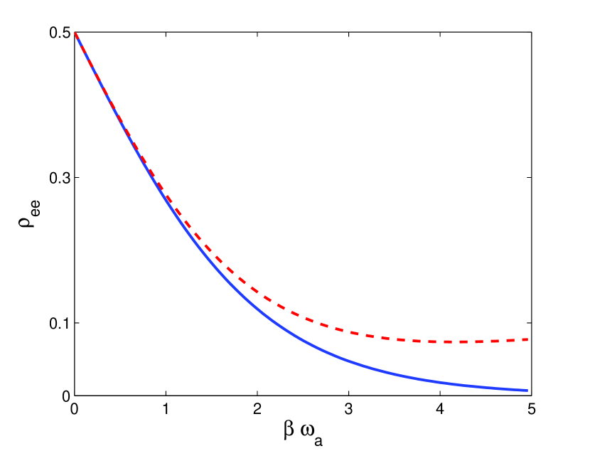
Figure 1: Excitation of the TLS at thermal equilibrium as a function of the inverse temperature $\beta$ either with (dashed) and without (solid) considering the effect of the system-bath interaction. Parameters: memory time of the bath $t_{c}=2/\omega_{a}$, peak of the Lorentzian bath spectrum $\omega_{0}=2\omega_{a}$, maximal coupling strength to the bath $|\eta_{max}|^{2}=\omega_{a}/100$, where $\hbar\omega_{a}$ is the energy separation of the TLS.

Using a similar analysis, the mean interaction energy to $O(\epsilon^{2})$, is given by

$$\langle H_{SB}(\epsilon)\rangle_{Eq}=-\hbar\omega_{a}\epsilon^{2}\\ \cdot\frac{\int^{\infty}_{-\infty}d\omega G_{T}(\omega)\left[P^{+}_{eq}\tilde{\mathcal{K}}^{+}(\omega)-P^{-}_{eq}\tilde{\mathcal{K}}^{-}(\omega)\right]}{1+\epsilon^{2}\int^{\infty}_{-\infty}d\omega G_{T}(\omega)\left[P^{+}_{eq}\mathcal{K}^{+}(\omega)+P^{-}_{eq}\mathcal{K}^{-}(\omega)\right]},$$ (13a)

where the quantity in brackets is dimensionless, and

$$\tilde{\mathcal{K}}^{\pm}=\frac{1}{1\mp\frac{\omega}{\omega_{a}}}\\ \cdot\big{[}\cosh\beta\hbar(\omega_{a}\mp\omega)-1\pm\sinh\beta\hbar(\omega_{a}\mp\omega)\big{]}.$$ (13b)

For a Lorentzian coupling spectrum,

$$\eta_{k}=\eta_{max}\sqrt{\frac{\Gamma^{2}}{\Gamma^{2}+(\omega_{0}-\omega_{k})^{2}}},$$ (14a)

the mean interaction-energy at $$T=0K$$, is simply given by the bath-induced lamb shift coh92

$$\langle H_{SB}\rangle_{Eq}\approx-\hbar\omega_{a}\int^{\infty}_{0}d\omega\frac{\Gamma^{2}}{\Gamma^{2}+(\omega_{0}-\omega)^{2}}\frac{1}{(1+\omega/\omega_{a})}.$$ (14b)

This proves the negativity of the mean system-bath interaction energy in equilibrium.

III Disturbance of equilibrium by impulsive QND measurement

The Hamiltonian is intermittently perturbed by the coupling of the system (qubit) to the detector (measuring apparatus), designed to effect a QND impulsive measurement in the $\sigma_{z}$-basis. Such a measurement projects the qubit onto the ${|e\rangle}$ or ${|g\rangle}$ energy states. We stress that the measurement results are unread, i.e., the qubit dynamics is changed by non-selective measurements.

III.1 Dynamic description of the measurement

The time-dependent system-detector coupling (to the $k$th detector) has the form

$$H_{SD}(t)=\frac{h(t)}{2}(1+\sigma_{z})\left({|0\rangle}{\langle 0|}+{|1\rangle}{\langle 1|}-{|0\rangle}{\langle 1|}-{|1\rangle}{\langle 0|}\right).$$ (15)

where $(1+\sigma_{z})={|e\rangle}{\langle e|}$ ensures QND measurement of the qubit energy, and

$$h(t)=\frac{\pi}{4\tau}\left({\rm tanh}^{2}\left(\frac{t-t_{0}}{\tau}\right)-1\right)$$ (16)

is a smooth temporal profile of the system coupling to the detector qubits during the measurement that occurs at time $t_{0}$ and has a duration of $\tau$.

The detector (ancilla) qubits have energy-degenerate states $|0\rangle,|1\rangle$ so that we may set the detector Hamiltonian to be zero

$$H_{D}=0.$$ (17)

This form of the single-measurement Hamiltonian $H_{SD}$ was chosen so that the measurement interval is $[0,\tau]$:

$$e^{-i\int_{0}^{\tau}dtH_{SD}(t)/\hbar}=U_{C}.$$ (18)

where $U_{C}$ denotes to the CNOT operation.

In our model (Eqs. (4) - (18))

$$e^{-i\int_{0}^{\tau}dtH_{SD}(t)}{|0\rangle}_{D}=U_{C}|0\rangle_{D}\\ ={|1\rangle}_{D}{|e\rangle}{\langle e|}+{|0\rangle}_{D}{|g\rangle}{\langle g|}.$$ (19)

The measurement consists in letting the TLS interact with the detector (a degenerate TLS) via $H_{SD}$. The measurement outcomes are averaged over (for non-selective measurements), by tracing out the detector degree of freedom. The total effect on the system density-operator is:

$$\rho_{S}\mapsto Tr_{D}\left\{U_{C}\rho_{S}\otimes{|0\rangle}_{DD}{\langle 0|}\right\}\\ ={|e\rangle}{\langle e|}\rho_{S}{|e\rangle}{\langle e|}+{|g\rangle}{\langle g|}\rho_{S}{|g\rangle}{\langle g|}$$ (20)

i.e., the diagonal elements are unchanged, and the off-diagonals are erased. Since the TLS is entangled with the bath, the effect of the measurement in Eq. (18) is:

$$\rho_{tot}(0)= \rho_{Eq}\rightarrow\rho_{tot}^{M}=Tr_{D}\left\{U_{C}\rho_{tot}\otimes{|0\rangle}_{DD}{\langle 0|}\right\}$$

$$= {|e\rangle}{\langle e|}\rho_{tot}{|e\rangle}{\langle e|}+{|g\rangle}{\langle g|}\rho_{tot}{|g\rangle}{\langle g|}$$

$$\equiv \rho^{B}_{ee}{|e\rangle}{\langle e|}+\rho^{B}_{gg}{|g\rangle}{\langle g|}.$$ (21)

Since $H_{SD}$ in Eq. (15) commutes with $H_{S}$, we may consider the measurement-induced evolution of ${\langle H_{SB}(\tau)\rangle}$, rather than ${\langle H_{tot}(\tau)\rangle}$. In the impulsive limit ($\tau\rightarrow 0$), the measurement yields:

$${\langle H_{SB}\rangle}_{EQ}\rightarrow{\langle H_{SB}(\tau)\rangle}^{M}\\ =Tr\left\{\rho_{tot}(0)\phantom{\rangle}_{D}{\langle 0|}U_{C}^{\dagger}H_{SB}(0)U_{C}{|0\rangle}_{D}\right\}.$$ (22)

Finally, using the RHS of (19) and (4), we get:

$$\phantom{\rangle}{}_{D}{\langle 0|}U_{C}^{\dagger}H_{SB}(0)U_{C}{|0\rangle}_{D}=0\\ \rightarrow{\langle H_{SB}(\tau)\rangle}^{M}=0.$$ (23)

In fact, this result follows immediately from the nature of the projective measurement:

$$\begin{split}\langle H_{SB}\rangle^{M}=&\frac{1}{2}\langle H_{SB}\rangle_{Eq}\\ &+\frac{1}{2}\sum_{k}\eta_{k}{\rm Tr}[(b_{k}+b^{\dagger}_{k})\sigma_{z}\sigma_{x}\sigma_{z}\rho_{Eq}]\\ =&\frac{1}{2}\langle H_{SB}\rangle_{Eq}-\frac{1}{2}\langle H_{SB}\rangle_{Eq}=0,\end{split}$$ (24)

where we have used the identity $\sigma_{z}\sigma_{x}\sigma_{z}=-\sigma_{x}$.

This expresses the vanishing of $Tr\left\{\rho_{tot}(\tau)H_{SB}\right\}^{M}$ due to the diagonality of $\rho_{tot}^{M}(\tau)$ with respect to $S$. Since $H_{D}=0$, the detector mean energy is not affected by the measurement.

III.2 Post-measurement heating

As shown in (III.1) above, a nearly-impulsive (projective) quantum measurement ($\tau\rightarrow 0$) of $S$, in the $|g\rangle,~{}|e\rangle$ basis, using the energy supplied by $H_{SD}(0<t<\tau)$ eliminates the mean system-bath interaction energy. Now the pre-measurement equilibrium mean value, ${\langle H_{SB}\rangle}_{Eq}$, is negative, as is shown above (Eq. (13a)) by second-order perturbation theory, provided the temperature is positive, i.e., the ${|g\rangle}$ state is populated more than the ${|e\rangle}$ state at thermal equilibrium. Hence

$$\begin{split}&{\langle H_{SB}(0)\rangle}_{Eq}<0\mapsto{\langle H_{SB}(\tau)\rangle}^{M}=0,\\ &{\langle H_{SD}(t)\rangle}=-{\langle H_{SB}(t)\rangle}^{M}.\end{split}$$ (25)

After the measurement (as $H_{SD}(t\geq\tau)=0$), time-energy uncertainty at $\Delta t\lesssim 1/\omega_{a}$ results in the breakdown of the RWA, i.e., $\langle H_{S}+H_{B}\rangle$ is not conserved as $\Delta t$ grows. The resulting ${\langle H_{S}\rangle}+{\langle H_{B}\rangle}$ changes stem from the non-commutativity of $H_{SB}$ and $H_{SD}$. Only $\langle H_{tot}\rangle$ is conserved, by unitarity, until the next measurement. Hence, the post-measurement decrease of $\langle H_{SB}\rangle$ with $\Delta t$, signifying the restoration of equilibrium:

$$\langle H_{SB}(\tau)\rangle^{M}=0\rightarrow\langle H_{SB}(\tau+\Delta t)\rangle<0,$$ (26)

is at the expense of the increase

$$\langle H_{S}+H_{B}\rangle=\langle H_{tot}\rangle-\langle H_{SB}\rangle>0,$$ (27)

i.e., heating of the system and the bath (Fig. 2,  3), combined.

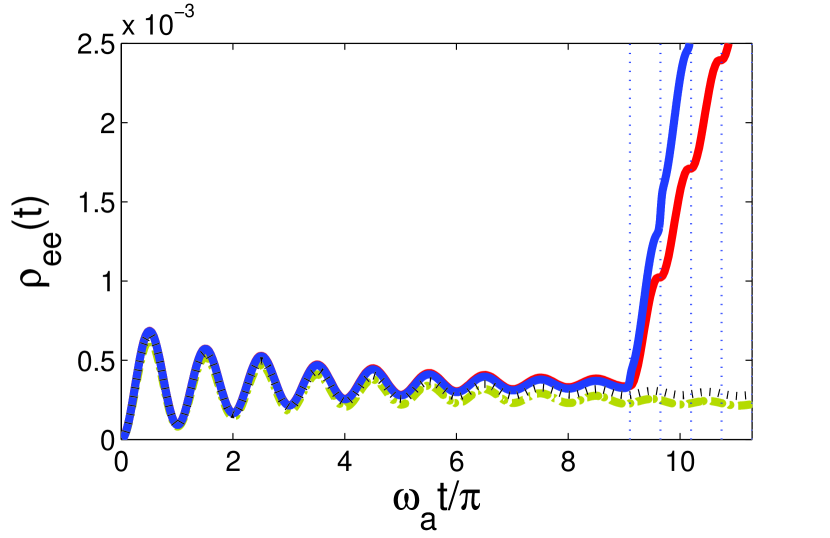
Figure 2: System evolution as a function of time. Excited-level population as a function of time for initially zero-temperature product state, followed by relaxation to quasi-equilibrium and then subjected to a series of measurements (vertical dashed lines). Measurements of finite duration ($\tau_{k}=0.11/\omega_{a}$) (blue line) results in somewhat larger heat-up than impulsive measurements (red line), but the dominant effect is the same for both. Observe the agreement between $2^{nd}$ order master equation (green), two-quanta exchange with a discrete bath, and exact numerical solution for a discrete bath of $40$ modes (black dashed). Parameters: memory time of the bath $t_{c}=10/\omega_{a}$, peak of the bath spectrum $\omega_{0}=\omega_{a}$, maximal coupling strength to the bath $|\eta_{max}|^{2}=0.07\omega_{a}$, where $\hbar\omega_{a}$ is the energy separation of the TLS.

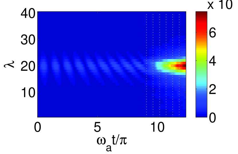
Figure 3: Excitations as a function of $t$ of the $40$ modes in the two-quanta model. $\lambda$ is the mode number. Parameters as in Fig. 2

III.3 Short-time post-measurement qubit evolution

Let us denote the even part of the bath state by $|B^{{\rm even}}\rangle|e\rangle$ and that of the odd part as $|B^{{\rm odd}}\rangle$, then:

$$|B^{{\rm even}}_{\bm{n},g}(t)\rangle\otimes|g\rangle+|B^{{\rm odd}}_{\bm{n},g}(t)\rangle\otimes|e\rangle\equiv|\Psi_{\bm{n},g}(t)\rangle.$$ (28)

Here $B^{{\rm even}}$ (respectively, $B^{{\rm odd}}$) is a combination of bath $\hat{N}$-eigenstates with eigenvalues differing from $\hat{N}$ by even (respectively, odd) numbers.

The post-measurement evolution of the system alone, described by $\rho_{S}=Tr_{B}\rho_{tot}$, is not at all obvious. Its Taylor expansion holds at short evolution times, $\Delta t\ll 1/\omega_{a}$,

$$\rho_{S}(\tau+\Delta t)\simeq\rho_{S}(\tau)+\Delta t\dot{\rho}_{S}(\tau)+\frac{\Delta t^{2}}{2}\ddot{\rho}_{S}(\tau)+\ldots$$ (29)

The $0$th order term is unchanged by the measurement, $\rho_{S}(\tau)=\rho_{S}(t\leq 0)$.

Due to the post-measurement vanishing of the off-diagonal elements of $\rho_{tot}$ (Eq. (21), for $\rho_{tot}(t)=|\Psi_{\bm{n},g}(t)\rangle\langle\Psi_{\bm{n},g}(t)|$ (Eq. (28)), we have

$$\begin{split}\left(\rho_{S}\right)_{eg}(t)=&{\langle e|}\rho_{S}(t){|g\rangle}=Tr_{B}\langle e|\rho_{tot}(t)|g\rangle\\ =&\langle B^{{\rm even}}_{\bm{n},e}(t)|B^{{\rm odd}}_{\bm{n},e}(t)\rangle=0\end{split}$$ (30)

Hence, $\rho_{S}$ is diagonal at any time $t$.

Its derivative immediately after the measurement, $\dot{\rho_{S}}(\tau)$, has the form:

$$\dot{\rho_{S}}(\tau)= -ie^{-i\omega_{a}\tau}{|e\rangle}{\langle g|}Tr_{B}\left\{\mathcal{B}\left(\rho_{gg}^{B}-\rho_{ee}^{B}\right)\right\}+H.C.$$

$$= 0.$$ (31)

The same argument goes through upon permuting $e\leftrightarrow g$ everywhere for $\rho_{tot}=|\Psi_{\bm{n},e}(t)\rangle\langle\Psi_{\bm{n},e}(t)|$.

Hence, the first derivative vanishes at $t=\tau(\Delta t=0)$ due to the definite parity of the bath density-operator correlated to ${|g\rangle}$ or ${|e\rangle}$. This post-measurement vanishing of the first derivative, $\dot{\rho}_{S}(\tau)=0$, is the condition for the quantum Zeno effect (QZE)mis77 ; kof00 ; kof04 ; facchi2001po . The time evolution of $\rho_{S}$ is then governed by its second time derivative $\ddot{\rho}_{S}(\tau)$.

For the factorisable thermal state,

$$\rho_{tot}=Z^{-1}e^{-\beta H_{0}}=Z_{B}^{-1}e^{-\beta H_{B}}Z_{S}^{-1}e^{-\beta H_{S}},$$ (32)

we have:

$$\begin{split}\rho^{B}_{ee}\equiv&\langle e|\rho_{tot}|e\rangle=\langle e|Z_{S}^{-1}e^{-\beta H_{S}}|e\rangle Z_{B}^{-1}e^{-\beta H_{B}}\\ =&\left(\rho_{S}\right)_{ee}\rho_{B}~{}({\rm and~{}}e\leftrightarrow g).\end{split}$$ (33)

For this $\rho_{tot}$, the second derivative of $\rho_{S}$ immediately after the measurement is (cf. Eq. (21))

$$\ddot{\rho}_{S}(\tau)=2\sigma_{z}Tr_{B}\left\{\mathcal{B}^{2}(\rho_{gg}^{B}-\rho_{ee}^{B})\right\}.$$ (34)

The scalar factor is positive:

$$Tr_{B}\left\{\hat{\mathcal{B}}^{2}\left(\rho^{B}_{gg}-\rho^{B}_{ee}\right)\right\}\\ =Tr_{B}\left\{\hat{\mathcal{B}}^{2}\rho_{B}\right\}\left(\left(\rho_{S}\right)_{gg}-\left(\rho_{S}\right)_{ee}\right)>0,$$ (35)

where we have used $Tr_{B}\{\rho^{B}_{gg(ee)}\}=\left(\rho_{S}\right)_{gg(ee)}$ which follows from the definition (Eq.(21)): $\rho^{B}_{ee(gg)}={\langle e(g)|}\rho_{tot}{|e(g)\rangle}$. The first factor in (35) is positive by virtue of the positivity of the operator $\hat{\mathcal{B}}^{2}$ ($\hat{\mathcal{B}}$ being Hermitian), and the second is positive iff there is no population inversion for the TLS.

Hence, the second derivative in (29) is positive shortly after the measurement, if there is no initial population inversion of the system, i.e., for non-negative temperature.

III.4 Post-measurement state

The combined (system- and bath-) equilibrium state satisfies:

$$\rho_{tot}^{M}=Z^{-1}e^{-\beta H_{tot}}=\rho_{tot}=Z^{-1}e^{-\beta\left(H_{0}+O(H_{SB}^{2})\right)}.$$ (36)

Thus, for sufficiently weak coupling, Eq. (33) dominates.

How is this reconciled with the non-unitary nature of the projection, whereby the mixedness of the total state must increase? Indeed,

$${\rm Tr}[(\rho^{M})^{2}]=\frac{1}{2}{\rm Tr}[(\rho_{Eq})^{2}]+\frac{1}{2}{\rm Tr}[(\sigma_{z}\rho_{Eq}\sigma_{z}\rho_{Eq})]$$ (37)

Yet, in the weak-coupling limit, the increase in mixedness due to measurement is $\cong O(\epsilon^{4})$ and hence can be neglected.

IV Post-measurement free evolution of the qubit

The evolution of $\rho_{S}$ at longer times (in the regime of weak system-bath coupling) may be approximately described (as verified by our exact numerical simulationsnest2003dqd ) by the second-order non-Markovian master equation (ME)breuer2002toq (Fig. 2). Higher-order corrections to the ME will be discussed elsewhere. The 2nd order ME for $\rho_{S}$, on account of its diagonality, can be cast into the following population rate equationskof04 , dropping the subscript $S$ in what follows and setting the measurement time to be $t=0$:

$$\dot{\rho}_{ee}(t)= -\dot{\rho}_{gg}(t)=R_{g}(t)\rho_{gg}-R_{e}(t)\rho_{ee},$$ (38)

$$R_{e(g)}(t)= 2\pi t\int_{-\infty}^{\infty}d\omega G_{T}(\omega){\rm sinc}\left[(\omega\mp\omega_{a})t\right].$$ (39)

Here ${\rm sinc}(x)=\frac{\sin(x)}{x}$. We shall assume that $G_{0}(\omega)$, the zero-temperature coupling spectrum, has peak coupling strength at $\omega_{0}$ and spectral width $\sim 1/t_{c}$.

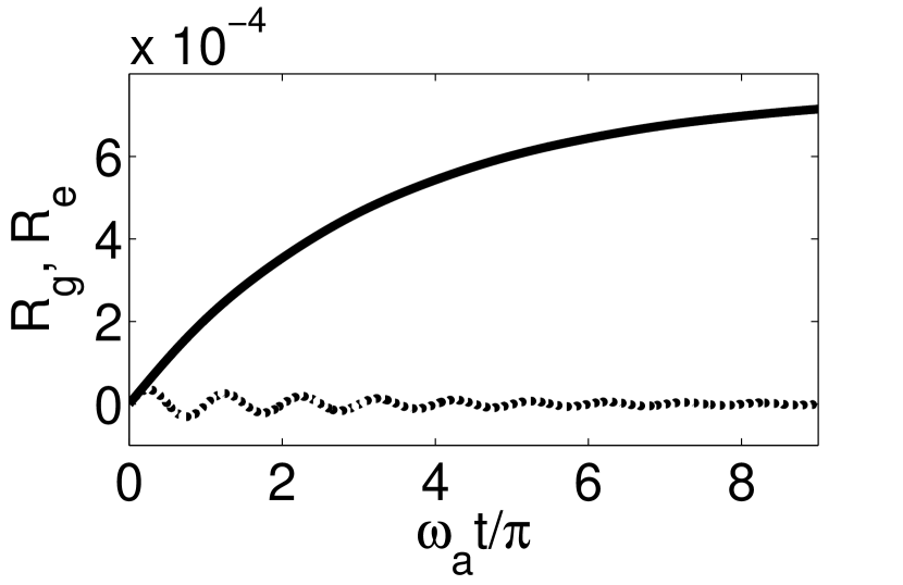
Figure 4: Relaxation rates, $R_{g}$ (dashed) and $R_{e}$ (solid) as a function of time. Parameters as in Fig. 2.

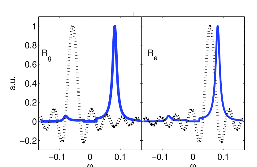
Figure 5: $R_{g}(t)$ and $R_{e}(t)$ (Eq. (39)) depicted as spectral overlaps of coupling spectrum (blue solid) and ${\rm sinc}((\omega\pm\omega_{a})t)$ (black dashed).

The entire dynamics is determined by $R_{e(g)}(t)$ (Figs. 4, 5), the relaxation rates of the excited (ground) states:

(i) At short times $t\ll 1/\omega_{a}\ll t_{c}$ the ${\rm sinc}$ function in (39) is much broader than $G_{T}$. The relaxation rates $R_{e}$ and $R_{g}$ are then equal at any temperature, indicating the complete breakdown of the RWA discussed above: $|g\rangle\rightarrow|e\rangle$ and $|e\rangle\rightarrow|g\rangle$ transitions do not require quantum absorption or emission by the bath, respectively. The rates $R_{e(g)}$ then become linear in time, manifesting the QZEkof00 ; facchi2001po ; kof04 :

$$R_{e(g)}(t\ll t_{c})\approx 2\dot{R}_{0}t,$$ (40)

$$\dot{R}_{0}\equiv\int_{-\infty}^{\infty}d\omega G_{T}(\omega)={\langle\mathcal{B}^{2}\rangle}.$$ (41)

This short-time regime entails the universal Zeno heating rate:

$$\frac{d}{dt}\left(\rho_{ee}-\rho_{gg}\right)\approx 4\dot{R}_{0}t(\rho_{gg}-\rho_{ee}).$$ (42)

(ii) At intermediate non-Markovian times, $t\sim 1/\omega_{a}$, when the ${\rm sinc}$ function and $G_{T}$ in (39) have comparable widths, the relaxation rates $R_{e(g)}(t)$ exhibit several unusual phenomena that stem from time-energy uncertainty. The change in the overlap of the ${\rm sinc}$ and $G_{T}$ functions with time results in damped aperiodic oscillations of $R_{e}(t)$ and $R_{g}(t)$, near the frequencies $\omega_{0}-\omega_{a}$ and $\omega_{0}+\omega_{a}$, respectively. This oscillatory time dependence that conforms neither to QZE nor to the converse AZE of relaxation speeduplan83 ; kof00 ; facchi2001po , will henceforth be dubbed the oscillatory Zeno effect (OZE). Due to the negativity of the ${\rm sinc}$ function between its consecutive maxima, we can have a negative relaxation rate, which is completely forbidden by the RWA. Since ${\rm sinc}\left[(\omega+\omega_{a})t\right]$ is much further shifted from the peak of $G_{T}(\omega)$ than ${\rm sinc}\left[(\omega-\omega_{a})t\right]$, $R_{g}(t)$ is more likely to be negative than $R_{e}(t)$ (Figs. 4, 5). Hence, $\rho_{gg}(t)$ may grow at the expense of $\rho_{ee}(t)$ more than allowed by the thermal-equilibrium detailed balance. This may cause transient cooling, as detailed below.

(iii) At long times $t\gg t_{c}$, the relaxation rates attain their Golden-Rule (Markov) valueskof04

$$R_{e(g)}(t\gg t_{c})\simeq 2\pi G_{T}(\pm\omega_{a}).$$ (43)

The populations then approach those of an equilibrium Gibbs state whose temperature is equal to that of the thermal bath (Fig. 2).

If we repeat this procedure often enough, the TLS will either increasingly heat up or cool down, upon choosing the time intervals $\Delta t_{k}$ to coincide with either peaks or troughs of the $\rho_{ee}$ oscillations, respectively. Since consecutive measurements affect the bath and the system differently, they may acquire different temperatures, which then become the initial conditions for subsequent QZE heating or OZE cooling, Fig. 6. The results are shown for both different and common (Fig. 7) temperatures of the system and the bath. Remarkably, the system may heat up solely due to the QZE, although the bath is colder, or cool down solely due to the OZE or AZE, although the bath is hotter. The bath may undergo changes in temperature and entropy too (Fig. 3).

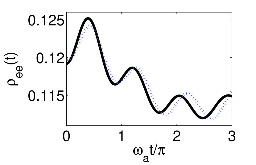
Figure 6: Example of a system experiencing first Zeno heating, then oscillatory-Zeno cooling, obtained from the second-order master equation (black-solid) and from the exact numerical solution for a discrete bath of 40 modes (blue dashed).

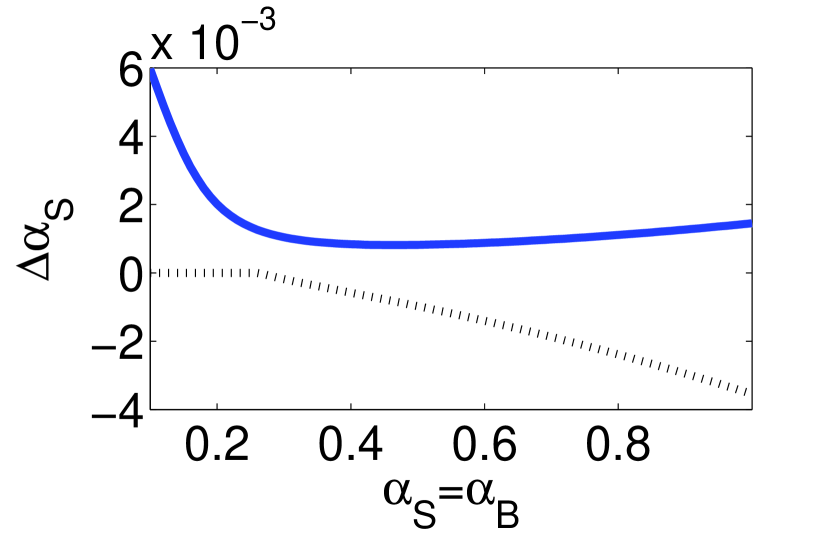
Figure 7: Maximal Zeno heating (blue solid) and subsequent maximal cooling (black dashed) as a function of common initial temperature of system and bath $\alpha_{S}=\alpha_{B}=\hbar\omega_{a}\beta$. Note the critical temperature for oscillatory-Zeno cooling. Parameters: memory time of the bath $t_{c}=10/\omega_{a}$, peak of the bath spectrum $\omega_{0}=\omega_{a}/0.7$, maximal coupling strength to the bath $|\eta_{max}|^{2}=4.36\omega_{a}$. These effects can be strongly magnified by choosing other suitable parameters.

V Derivation of cooling conditions

By integrating Eq. (39) over time to acquire $J_{g(e)}(t)$, one arrives at the following result:

$$J_{g}(t)=\int_{0}^{\infty}d\omega G_{0}(\omega)n_{T}(\omega){\rm sinc}^{2}((\omega-\omega_{a})t)\\ +\int_{0}^{\infty}d\omega G_{0}(\omega)(n_{T}(\omega)+1){\rm sinc}^{2}((\omega+\omega_{a})t)$$ (44)

$$J_{e}(t)=\int_{0}^{\infty}d\omega G_{0}(\omega)n_{T}(\omega){\rm sinc}^{2}((\omega+\omega_{a})t)\\ +\int_{0}^{\infty}d\omega G_{0}(\omega)(n_{T}(\omega)+1){\rm sinc}^{2}((\omega-\omega_{a})t)$$ (45)

To obtain cooling below the equilibrium temperature, one requires that:

$$\frac{J_{e}(t)}{J_{g}(t)}>\frac{J_{e}^{Eq}}{J_{g}^{Eq}}=\frac{R_{e}^{Eq}}{R_{g}^{Eq}}=\frac{n(\omega_{a})}{n(\omega_{a})+1}$$ (46)

Rearranging the terms in the above equation, gives the cooling condition,

$$\begin{split}&\int_{0}^{\infty}G_{0}(\omega)\frac{\sin^{2}\left[\frac{t}{2}(\omega-\omega_{a})\right]}{(\omega-\omega_{a})^{2}}(n_{T}(\omega_{a})-n_{T}(\omega))\\ >&\int_{0}^{\infty}G_{0}(\omega)\frac{\sin^{2}\left[\frac{t}{2}(\omega+\omega_{a})\right]}{(\omega+\omega_{a})^{2}}(n_{T}(\omega_{a})+n_{T}(\omega)+1)\end{split}$$ (47)

A general quest for finding the spectral density function $G_{0}(\omega)$,which satisfies the above condition in some time interval, at any given temperature $T$, is quite difficult. In the high temperature limit i.e., $n_{T}(\omega)>>1$ one can find a necessary condition on the peak position of $G_{0}(\omega)$, which can satisfy the above inequality. Substituting the high-temperature limit for $n_{T}(\omega)\simeq 1/\beta\omega$, one can show that in order to allow cooling $G_{0}(\omega)$ needs to be concentrated in the frequency interval defined by

$$\omega_{a}<\omega<\Omega,$$ (48)

where

$$\beta\Omega=1+\frac{\beta\omega_{a}+\sqrt{4+12\beta\omega_{a}+\beta^{2}\omega_{a}^{2}}}{2}.$$ (49)

Though $\beta\Omega>1$, it is only the maximum possible bound on the detuning of the bath spectrum for the qubit frequency, indicating that one should not detune the bath spectrum too far from $\omega_{a}$ to see the cooling effect. We have numerically verified these conditions for various bath coupling spectrums. In the same spirit one can find regions in frequency space, where for specific times there will be no cooling, independent of the shape of $G_{0}(\omega)$.

VI Entropy dynamics

One may always define the entropy of $\rho_{S}$ relative to its equilibrium state $\rho_{0}$ (“entropy distance”) and the negative of its rate of change, asali79 ; lin74 :

$$\bm{S}(\rho_{S}(t)||\rho_{0})\\ \equiv\mathrm{Tr}\{\rho_{S}(t)\ln\rho_{S}(t)\}-\mathrm{Tr}\{\rho_{S}(t)\ln\rho_{0}\}$$ (50)

$$\bm{\sigma}(t)\equiv-\frac{d}{dt}\bm{S}(\rho_{S}(t)||\rho_{0}).$$ (51)

In the Markovian realm $\bm{\sigma}(t)\geq 0$spo78 ; ali79 ; lin74 is a statement of the second law of thermodynamics. Since $\rho_{S}$ is diagonal, it follows that $\bm{\sigma(t)}$ is positive iff $\frac{d}{dt}\left|\rho_{ee}(t)-(\rho_{0})_{ee}\right|\leq 0$, consistently with the interpretation of the relative entropy $\bm{S}(\rho_{S}||\rho_{0})$ in (51) as the entropic “distance” from equilibrium. Conversely, whenever the oscillatory $\rho_{ee}(t)$ drifts away from its initial or final equilibria, $\bm{\sigma}$ takes negative values (Fig. 8).

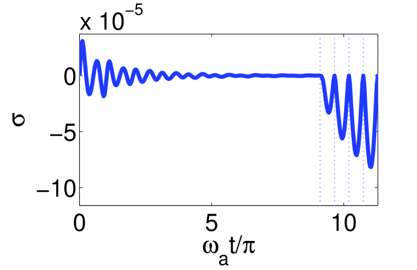
Figure 8: ${\bm{\sigma}}(t)$ (negative of relative entropy rate of change). Parameters as in Fig. 2.

VII Discussion: realization and practical consequences

Consider atoms or molecules in a microwave cavity (Fig. 9(a)) with controllable finite-temperature coupling spectrum $G_{T}(\omega)$ centered at $\omega_{0}$. Measurements can be effected on such a TLS ensemble with resonance frequency $\omega_{a}$ in the microwave domain, at time intervals $\Delta t_{k}\sim 1/(\omega_{0}\pm\omega_{a})$, by an optical QND probebraginsky1995qm at frequency $\omega_{p}\gg\omega_{a},\omega_{0}$. The probe pulses undergo different Kerr-nonlinear phase shifts $\Delta\phi_{e}$ or $\Delta\phi_{g}$ depending on the different symmetries (e.g., angular momenta) of $|e\rangle$ and $|g\rangle$. The relative abundance of $\Delta\phi_{e}$ and $\Delta\phi_{g}$ would then reflect the ratio $\rho_{ee}(t_{k})/\rho_{gg}(t_{k})$. Such QND probing may be performed with time-duration much shorter than $\omega_{a}^{-1}$, i.e. $\omega_{a}\tau_{k}\ll 1$, without resolving the energies of $|e\rangle$ and $|g\rangle$.

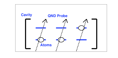
(a) Atoms in microwave cavity

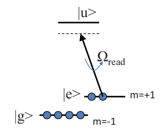
(b) Energy level description

Figure 9: Possible experimental setup

An experimental scenario involves collective N-atom coupling to near-resonant RF resonator (Fig. 9(a)). Let us choose ground sublevels ${|m=-1\rangle}\equiv{|g\rangle},{|m=+1\rangle}\equiv{|e\rangle}$, with Zeeman splitting $\omega_{eg}\cong MHz$. The collective Rabi frequency of $N\geq 10^{8}$ atoms at a cavity antinode is $N^{1/2}\Omega_{eg}/2\pi\cong 100KHz$. An optical beam will rotate in polarization (Fig. 9(b)), thus performing QND measurement (readout) that resolves ${|g\rangle}$ and ${|e\rangle}$ (by their symmetry, not by energy) if its Rabi frequency:

$$\Omega_{\rm read}\cong N^{1/2}(\Omega_{0})_{read}^{2}/\Delta\geq\omega_{eg}.$$ (52)

Such a Rabi frequency corresponds to RWA violation, as discussed in the text above.

Non-selective measurements increase the Von-Neumann entropy of the detector ancillae. Since our ancillae are laser pulses, they are only used once and we may progressively change the TLS ensemble thermodynamics by consecutive pulses, disregarding their entropic or energetic price.

VIII Conclusions

To conclude, we have shown that frequent QND measurements may induce either anomalous heating or anomalous cooling of TLS coupled to baths on non-Markovian time scales. These findings defy the standard notions of quantum thermodynamics regarding system equilibration in the presence of a thermal bath.

The practical advantage of the predicted anomalies is the possibility of very rapid control of cooling and entropy, which may be attained after several measurements at $t\geq\omega_{a}^{-1}$ and is only limited by the measurement rate. By contrast, conventional cooling requires much longer times, $t\gg t_{c}$, to reach thermal equilibrium.

References

- (1) LD. Landau, EM. Lifshitz, Statistical Physics, part 1, third ed., Pergamon Press, 1980.
- (2) H. Spohn, Entropy production for quantum dynamical semigroup, J. Math. Phys. 19 (1978) 1227.
- (3) R. Alicki, The quantum open system as a model of the heat engine, J. Phys. A 12 (1979) L103.
- (4) C. Jarzynski, Nonequilibrium equality for free energy differences, Phys. Rev. Lett. 78 (1997) 2690.
- (5) G. Lindblad, Expectations and entropy inequalities for finite quantum systems, Comm. Math. Phys. 39 (1974) 111–119.
- (6) LS Schulman, B. Gaveau, Ratcheting Up Energy by Means of Measurement, Phys. Rev. Lett. 97 (2006) 240405.
- (7) J. Piilo, S. Maniscalco, K.A. Suominen, Quantum Brownian motion for periodic coupling to an Ohmic bath, Phys. Rev. A 75 (2007) 32105.
- (8) Th. M. Nieuwenhuizen, A. E. Allahverdyan, Statistical thermodynamics of quantum Brownian motion: Construction of perpetuum mobile of the second kind, Phys. Rev. E 66 (2002) 036102.
- (9) Noam Erez, Goren Gordon, Mathias Nest, Gershon Kurizki, Thermodynamic control by frequent quantum measurements, Nature 452 (2008) 724.
- (10) C. Cohen-Tannoudji, J. Dupont-Roc, G. Grynberg, Atom-Photon Interactions, Wiley, New York, 1992.
- (11) A. G. Kofman, G. Kurizki, Unified theory of dynamically suppressed qubit decoherence in thermal baths, Phys. Rev. Lett. 93 (2004) 130406.
- (12) S. P. Heims, E. T. Jaynes, Theory of gyromagnetic effects and some related magnetic phenomena, Rev. Mod. Phys. 34 (1962) 143–165.
- (13) B. Misra, E. C. G. Sudarshan, Zeno’s paradox in quantum theory, J. Math. Phys. 18 (1977) 756–763.
- (14) A. G. Kofman, G. Kurizki, Acceleration of quantum decay processes by frequent observations, London Nature 405 (2000) 546–550.
- (15) P. Facchi, S. Pascazio, Quantum Zeno and inverse quantum Zeno effects, Progress in Optics 42 (2001) 147.
- (16) M. Nest, H.D. Meyer. Dissipative quantum dynamics of anharmonic oscillators with the multiconfiguration time-dependent Hartree method, J. Chem. Phys. 119 (2003) 24.
- (17) H.P. Breuer, F. Petruccione, The theory of open quantum systems, Oxford University Press New York, 2002.
- (18) A. M. Lane, Decay at early times - larger or smaller than the golden rule, Phys. Lett. A 99 (1983) 359–360.
- (19) V.B. Braginsky, F.Y. Khalili, Quantum Measurement, Cambridge University Press, 1995.