Probing the excitation of extreme starbursts: High resolution mid-IR spectroscopy of Blue Compact Dwarfs

Lei Hao ¹¹affiliation: University of Texas at Austin, McDonald Observatory, 1 University Station, C1402, Austin, Texas 78712-0259 , Yanling Wu²²affiliation: Caltech, Infrared Processing and Analysis Center, MC 314-6, Pasadena, CA 91125 , V. Charmandaris³³affiliation: University of Crete, Department of Physics, P. O. Box 2208, GR-71003, Heraklion, Greece ⁴⁴affiliation: IESL/Foundation for Research & Technology - Hellas, GR-71110, Heraklion, Greece, and Chercheur Associé, Observatoire de Paris, F-75014, Paris, France , H. W. W. Spoon⁵⁵affiliation: Cornell University, Astronomy Department, Ithaca, NY 14853-6801 , J. Bernard-Salas⁵⁵affiliation: Cornell University, Astronomy Department, Ithaca, NY 14853-6801 , D. Devost⁶⁶affiliation: CFHT:Canada France Hawaii Telescope, Kamuela, HI, 96743, USA. , V. Lebouteiller⁵⁵affiliation: Cornell University, Astronomy Department, Ithaca, NY 14853-6801 , J. R. Houck⁵⁵affiliation: Cornell University, Astronomy Department, Ithaca, NY 14853-6801 haol@astro.as.utexas.edu

Abstract

We present an analysis of the mid-infrared emission lines for a sample of 12 low metallicity Blue Compact Dwarf (BCD) galaxies based on high resolution observations obtained with Infrared Spectrograph on board the Spitzer Space Telescope. We compare our sample with a local sample of typical starburst galaxies and active galactic nuclei (AGNs), to study the ionization field of starbursts over a broad range of physical parameters and examine its difference from the one produced by AGN. The high-ionization line [OIV]25.89 $\mu$ m is detected in most of the BCDs, starbursts, and AGNs in our sample. We propose a diagnostic diagram of the line ratios [OIV]25.89 $\mu$ m/[SIII]33.48 $\mu$ m as a function of [NeIII]15.56 $\mu$ m/[NeII]12.81 $\mu$ m which can be useful in identifying the principal excitation mechanism in a galaxy. Galaxies in this diagram split naturally into two branches. Classic AGNs as well as starburst galaxies with an AGN component populate the upper branch, with stronger AGNs displaying higher [NeIII]/[NeII] ratios. BCDs and pure starbursts are located in the lower branch. We find that overall the placement of galaxies on this diagram correlates well with their corresponding locations in the log([NII]/H $\alpha$ ) vs. log([OIII]/H $\beta$ ) diagnostic diagram, which has been widely used in the optical. The two diagrams provide consistent classifications of the excitation mechanism in a galaxy. On the other hand, the diagram of [NeIII]15.56 $\mu$ m/[NeII]12.81 $\mu$ m vs. [SIV]10.51 $\mu$ m/[SIII]18.71 $\mu$ m is not as efficient in separating AGNs from BCDs and pure starbursts. Our analysis demonstrates that BCDs in general do display higher [NeIII]/[NeII] and [SIV]/[SIII] line ratios than starbursts, with some reaching values even higher than those found at the centers of AGNs. Despite their hard radiation field though, no [NeV]14.32 $\mu$ m emission has been detected in the BCDs of our sample.

Subject headings:

dust, extinction – infrared: galaxies – galaxies: dwarf – galaxies: starburst – galaxies: active – galaxies: abundances

1. Introduction

Starburst galaxies are hosts of intense star formation activity with star formation rates (SFR) more than a factor of 3 compared to the Milky Way (SFR $>$ 10M_⊙yr^-1). The stellar population of the starbursts, especially the number of massive stars and the slope of the initial mass function (IMF), directly affect the hardness of the ionization field in the interstellar medium (ISM). Therefore, ratios of emission lines of different excitation levels are powerful tools to study the properties of the ionization field and to infer the stellar population of the starbursts. Infrared emission-line ratios are of particular interest and have been explored extensively with the Infrared Space Observatory (i.e. Thornley et al., 2000; Förster Schreiber et al., 2001; Verma et al., 2003, 2005), as the active star forming regions in the disks of starburst galaxies and circumnuclear regions are often optically obscured by dust. As a result, the emitted radiation, originating from a massive starburst and/or an accreting active nucleus, is emerging in the mid-infrared (mid-IR) (see Vacca et al., 2002; Gorjian et al., 2001) and far-IR. The advent of the Spitzer Space Telescope with its improved sensitivity opens new avenues in this direction, enabling detailed studies of large samples of quiescent and star forming galaxies (Dale et al., 2006, 2009; O’Halloran et al., 2008; Bernard-Salas et al., 2009), as well as more complex dust enshrouded infrared luminous sources which often host an active galactic nucleus (AGN) (Armus et al., 2007; Farrah et al., 2007).

Estimating the hardness of the ionization field plays a key role in determining the dominant power source at the centers of galaxies. Nuclear starbursts and accreting super-massive black holes (SMBH) are often intertwined and coexist, as best demonstrated in the case of Ultra Luminous Infrared Galaxies (ULIRGs)(see e.g. Genzel et al., 1998; Armus et al., 2007, and references therein). The radiation of an AGN, produced from the accretion of gas and stars onto the SMBH, has a much harder spectrum compared to the one produced by the massive young stellar populations. Therefore, the hardness of the radiation field has been a key parameter addressed by previous diagnostic methods to determine the energy source in galaxies (e.g. Baldwin et al., 1981; Veilleux & Osterbrock, 1987; Genzel et al., 1998; Laurent et al., 2000; Nardini et al., 2008).

In the study of the ionization field of galaxies with massive starbursts, the case of low-metallicity Blue Compact Dwarfs (BCDs) is particularly interesting. BCDs are galaxies characterized by their blue optical colors (M_B $<$ -18 mag), small linear sizes ( $<$ 1kpc) and low luminosities (Thuan & Martin, 1981; Gil de Paz et al., 2003). Even though BCDs are defined based on their morphological properties, they have been ubiquitously found to have low oxygen abundances as measured from the ionized gas in HII regions.

It is well established that the hardness of the stellar radiation increases with decreasing metallicity (e.g. Campbell et al., 1986). As a result, the ionization field of BCDs is generally much harder compared to a typical starburst. It is also known that the mass of a super massive black hole (SMBH) is correlated with the mass of the bulge of the host galaxy (Magorrian et al., 1998; Gebhardt et al., 2000; Ferrarese & Merritt, 2000) while only a fraction of the most massive SMBH are actively emitting radiation as a result of mass accretion (Hao et al., 2005b). BCDs in general are not massive enough to host such an active SMBH, with possibly only a few exceptions (see Izotov et al., 2007; Izotov & Thuan, 2008). Consequently, the excitation mechanism for the hard radiation field in BCDs is likely significantly different from the one responsible for the radiation field produced by an AGN. Furthermore, unlike starburst galaxies which are often obscured by dust, an analysis of a large sample of BCDs suggests that in BCDs nearly always the young massive stars which ionize the interstellar medium are easily detected and their dust extinction measured from the optical Balmer lines is typically fairly low (Wu et al., 2008b). There might be exceptions indicated from the mid-IR observations, with SBS0335-052E as the most extreme case. However, this is rather a unique galaxy and deviates from the usual trends seen in BCDs for different reasons as discussed in detail by Houck et al. (2004b). Understanding the differences in the excitation mechanism between BCDs and AGNs can provide insightful clues to decipher the power source in a starburst galaxy also hosting an AGN. Identifying those differences from the mid-IR spectral features is one of the main motivations behind the present work.

BCDs are often much fainter than typical starburst galaxies in the infrared. Up until the launch of the Spitzer Space Telescope (Werner et al., 2004), studies of starburst galaxies in the IR have included only a handful of BCDs (Lutz et al., 1998; Thornley et al., 2000; Verma et al., 2003; Madden et al., 2006). The superb sensitivity of the Spitzer allows us to observe a large sample of BCDs (see Wu et al., 2006, 2008a). In this paper, we provide the ionized gas diagnostic analysis of the low metallicity BCDs accessible to the high-resolution modules of the Infrared Spectrograph (IRS, Houck et al., 2004a). In addition, we contrast the BCD sample with typical starbursts and AGNs, to probe the excitation mechanism in these types of objects and understand where the difference comes from.

In §2, we introduce the sample and the data reduction method. In §3, we study the high-ionization emission lines, and propose a new diagnostic diagram to determine the energy source in a galaxy. In §4, we focus on other infrared emission lines and compare various excitation diagnostic diagrams of starbursts and BCDs. Our findings are summarized in §5.

2. Sample and Data Reduction

2.1. The BCD sample

We have compiled a sample of 12 BCDs and observed them in starring mode with the high-resolution modules (short-high, SH: 4.7 $\arcsec$ $\times$ 11.3 $\arcsec$ and long-high, LH: 11.1 $\arcsec$ $\times$ 22.3 $\arcsec$ ) of the IRS as part of the instrument team’s Guaranteed Time Observation (GTO) programs. The galaxies were drawn from the sample of Wu et al. (2006). We exclude Tol1214-277 as it is too faint and its high-resolution spectrum has low signal-to-noise ratio. We also exclude CG0752, CG0563, and CG0598 as they do not show typical BCD signatures. The characteristics of individual objects in the sample and analysis based on their Spitzer low-resolution spectra are presented in Wu et al. (2006, 2008a, 2008b).

The high-resolution module slits were centered on the nucleus of each galaxy, as was the case of the low-resolution observations (Wu et al., 2006). The data were processed by the Spitzer Science Center (SSC) data reduction pipeline version 13.2. Individual pointings to each nod position of the slit were co-added. The median of the combined images were extracted using the full slit extraction method of the IRS data analysis package SMART (Higdon et al., 2004). Then the extracted spectra were flux calibrated by multiplying them with a relative spectral response function (RSRF), which was created from the IRS standard star, $\xi$ Dra, for which accurate templates were available (Cohen et al., 2003). Note that emission from the sky background has not been subtracted from our spectra due to the lack of dedicated sky observations, thus discontinuity exists in some source spectra between SH and LH, however, this will not affect the results of our analysis since our conclusions are based on ratios of emission lines observed in the same module.

In the Appendix, we include close up plots of strong and weak emission lines visible in the IRS high-resolution spectra of BCDs. In order to measure the line strengths, a Gaussian profile is fitted to the lines above a local continuum fitted by an one-order polynomial. The [OIV]25.89 $\mu$ m and [FeII]25.99 $\mu$ m are close to each other and they are fit together using a two-Gaussian profile with fixed rest-frame wavelengths. The measured line strengths for the BCD sample are listed in Table 1. The errors are estimated based on the error propagation of the Gaussian fit assuming the error of the flux as the root mean square ( $rms$ ) of the continuum fit. Note that this does not take into account all the systematic uncertainties, especially the flux calibration. We estimate these to be 5% and choose it as our minimum uncertainty. The upper-limits are obtained by measuring the flux of a Gaussian with a height three times the local $rms$ , and with a FWHM equal to the instrumental resolution.

No extinction correction has been performed in our analysis. The corrections are typically minor for mid-IR fine-structure line ratios, except for ratios involving lines found close to the silicate features, such as the [SIV]10.51 $\mu$ m line. In the analysis of diagrams involving the [SIV] line (see Figure 9), we provide arrows indicating the effects of an A_V=30 mag of extinction, assuming a uniform dust screen and a Li & Draine (2001) extinction curve (see Farrah et al., 2007).

2.2. The Starburst and AGN sample

In order to study the ionization field of starbursts over a broad range of physical properties, we also examine a sample of 24 local starbursts observed in staring mode with the IRS high-resolution modules. The details of the sample, their high-resolution spectra and line measurements are described in Bernard-Salas et al. (2009). It should be emphasized that even though we broadly use the term “starburst” when referring to them, some may also have a weak AGN component.

In addition, we created a comparison sample of typical AGNs to investigate how the difference in the excitation mechanism of the gas, namely the radiation produced by an accretion disk versus massive young star formation, is reflected in the mid-IR emission lines. It is not our intention to have an AGN sample that is complete, but rather one that is representative of typical AGNs. Hence, we choose bona-fide AGNs, with no ambiguity in their classification, where the nuclear emission is known to dominate the integrated spectra of their host galaxies. We select from the Type 1 sources (Quasars and Seyfert 1s) used in Hao et al. (2007) for which IRS high-resolution observations are available. We also examine the strength of the Polycyclic Aromatic Hydrocarbon (PAH) emission in their mid-IR spectra and exclude sources with strong PAH features, since this would suggest a significant contribution from star forming regions in the disk of the host galaxy. Among those sources with weak PAH emission, we choose 10 AGNs that show strong mid-IR emission lines, in order to obtain the best S/N possible in our measurements. The AGN IRS spectra were extracted and the emission lines measured in the same way as the BCDs (see §2.1).

Furthermore, whenever applicable, we also compare the properties of emission lines in BCDs with those in low-redshift ULIRGs as well as HII regions found in our Galaxy, and in the Large and Small Magellanic Clouds (LMC/SMC). The sample and line measurements of the low-redshift ULIRGs are taken from Farrah et al. (2007), and the HII region data from Peeters et al. (2002) and Lebouteiller et al. (2008).

3. High-Ionization Emission Lines Diagnostics

3.1. The [OIV]25.89 $\mu$ m Emission

The IRS high-resolution spectra of BCDs are rich in fine-structure emission lines. All BCDs display strong [NeIII]15.56 $\mu$ m, [SIII]18.71 $\mu$ m, and [SIV]10.51 $\mu$ m emission. The [NeII]12.81 $\mu$ m line is well detected in about half of the BCD sample, but it is not seen in SBS0335-052E, Tol65, and VIIZw403. In the comparison samples of starbursts and AGNs, all these lines are strong and we discuss their relative flux ratios in §4.

The presence of high-ionization emission lines is of great interest, since their excitation often requires extreme conditions. One particular case is the [OIV]25.89 $\mu$ m line which has an ionization potential (IP) of 54eV, just above the HeII edge, and therefore it cannot be readily generated in the HII regions surrounding main-sequence stars. However, the [OIV] line had already been detected in several starburst galaxies with ISO (see Lutz et al., 1998). A possible explanation for this was that the [OIV] emission is due to a dust enshrouded AGN as the hard radiation field produced by the AGN can easily provide the energy needed to ionize O³⁺. However, Lutz et al. (1998) showed that at least in some starburst systems (such as the outer regions of M82), the [OIV] cannot be attributed to a weak AGN. Instead it must be due to either very hot stars, such as the Wolf-Rayet (WR) stars (see also Schaerer & Stasińska, 1999) or to the ionizing shocks associated with the starburst activity.

With the superb sensitivity of the Spitzer Space Telescope, we now find that the [OIV] line is fairly common in our BCD sample as well as the comparison sample of starburst galaxies. We detected [OIV] emission in 8 of the 12 BCDs, and in 21 of the 24 starbursts (see Bernard-Salas et al., 2009). This is very interesting since, as we will discuss in the following sessions, line ratios involving [OIV] provide a good diagnostic tool for identifying the presence of an AGN (see also Genzel et al., 1998; Armus et al., 2007).

3.2. The [OIV]/[SIII] vs. [NeIII]/[NeII] diagram

Refer to caption — Figure 1.— A plot of the [OIV]25.89 $\mu$ m/[SIII]33.48 $\mu$ m as a function of [NeIII]15.56 $\mu$ m/[NeII]12.81 $\mu$ m, for BCDs (diamonds), starbursts (squares), AGNs (crosses), and ULIRGs (plus signs). A circle around a symbol indicates that [NeV]14.32 $\mu$ m emission has been detected, while a filled symbol implies that this galaxy also has been classified as a Wolf-Rayet (WR) in the optical (see §3.4). The error bars of the line ratios in this and all subsequent plots are similar to the symbol size. The galaxies appear to be localized on two branches. One branch consists mainly of AGNs, or starbursts/ULIRGs hosting an AGN, while the other mainly contains BCDs or pure starburst galaxies. Two dashed lines are drawn as a guide to identify the two branches.

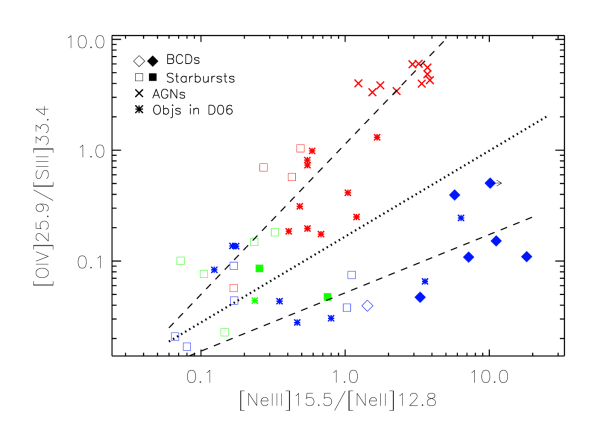
In Figure 1, we plot the line ratios of [OIV]25.89 $\mu$ m/[SIII]33.48 $\mu$ m as a function of [NeIII]15.56 $\mu$ m/[NeII]12.81 $\mu$ m for our BCDs, starburst galaxies AGNs and ULIRGs. We choose to use the line ratio of [OIV]25.89 $\mu$ m and [SIII]33.48 $\mu$ m because of their large difference in the ionization potential, and the absence of aperture effects, as both lines reside in the same IRS long-high module (see also Figure 3 in Genzel et al. 1998) . We use the [NeIII]/[NeII] line ratio as the other variable, as it is commonly used as an indicator of the strength of the EUV radiation field (e.g. Lutz et al., 1998; Thornley et al., 2000; Verma et al., 2003). Since both [NeIII] and [NeII] lines are of the same element, the ratio is independent of the gas abundance. We clearly see that the [OIV]/[SIII] ratio separates AGNs from BCDs, with AGNs having in general a factor of 10 higher [OIV]/[SIII] ratios than BCDs, even though they have similar [NeIII]/[NeII] ratios. Starburst galaxies display smaller [NeIII]/[NeII] ratios than AGNs and BCDs, but their values of the [OIV]/[SIII] ratio vary. In particular, it appears that starburst galaxies populate two branches with a common origin (the dashed lines in Figure 1), one pointing towards the locus of AGNs and the other to the BCDs. Among the starburst galaxies, Mrk266, NGC1365, NGC2623, NGC4194, NGC4945, NGC520, NGC660, NGC253, NGC1614, NGC1097, NGC3079, NGC4676, and NGC7252 are located in the upper branch reaching to the AGN locus, while NGC1222, NGC2146, NGC3256, NGC3310, NGC3628, NGC4088, and NGC7714 are in the lower branch that ties to the BCDs. The galaxies IC342, NGC3556, and NGC4818 have no detected [OIV] emission and their upper limits are indicated with arrows on the plot.

Given that the gas in AGNs and BCDs is excited by distinctly different physical mechanisms, the fact that they are found at the corresponding ends of the two branches of the diagram, also suggests that the excitation mechanisms leading to the [OIV] line emission in starbursts galaxies populating the two branches is different. This could be understood if the mid-IR emission of starbursts in the upper branch is due to some AGN component, while in starbursts of the lower branch is only due to the reprocessing of pure stellar radiation. Therefore, such a diagram can be used as a diagnostic tool to determine the origin of the dust enshrouded energy source in star forming galaxies. Interestingly, among the starbursts located in the upper branch, six also have detected [NeV]14.32 $\mu$ m emission (see Bernard-Salas et al., 2009), which has an IP of 97eV and is a clear AGN indicator. Five galaxies (NGC520, NGC253, NGC1614, NGC4676 and NGC7252) which do not have a confirmed AGN signature so far, are located in the lower left corner of the plot, where the two branches merge. Since at this area of the plot classification is more ambiguous, it is possible that a weak AGN component could be present, even though its [NeV] emission is too weak to be detected.

Unfortunately, in most of the ULIRGs with available IRS high resolution spectroscopy, their [SIII]33.48 $\mu$ m emission lines are redshifted out of the wavelength coverage of the IRS (see Farrah et al., 2007). Among the 10 ULIRGs that have both [OIV]25.89 $\mu$ m and [SIII]33.48 $\mu$ m detected, 9 are located on the upper branch and they all have detected [NeV] emission. IRAS09022-3615 is the only ULIRG with no [NeV] detection and it is located between the two branches. This is again consistent with the assertion that star forming galaxies with an AGN component do follow the upper branch.

The lower branch of the diagram seems to be populated by sources in which the ionizing radiation is due only to stellar photospheres. In addition to the BCDs, the pure starburst galaxies NGC7714, NGC3310, and NGC1222 (e.g. Brandl et al., 2004; Wehner et al., 2006; Beck et al., 2007) are located in the lower branch before the two branches merge. Moving along the branch towards higher values of the [NeIII]/[NeII] ratio, the metallicity overall decreases (see §4). The harder radiation field produced by the low metallicity environment strongly increases the [NeIII]/[NeII] ratio (by up to a factor of 100), but increases only moderately the [OIV]/[SIII] ratio (by a factor of 10). This was also noticed by Lutz et al. (1998), who indicated that low-metallicity dwarfs exhibit relatively stronger [OIV] than low-excitation starbursts, but the effect is not very pronounced compared to the large excitation difference as measured by the [NeIII]/[NeII]. One galaxy with a detected [NeV] emission (NGC3628, see Bernard-Salas et al., 2009) is on the lower branch. We note though that its location is also at the far left where the two branches merge, and as a result it does not contradict our bifurcation scheme.

As with the [NeIII]/[NeII] ratio, the ratio of [SIV]10.51 $\mu$ m/[SIII]18.71 $\mu$ m has also been widely used as a probe of the hardness of the ionization field. When plotting the [OIV]25.89 $\mu$ m/[SIII]33.48 $\mu$ m as a function of the [SIV]/[SIII] line ratio, we observe a similar bifurcation signature (see Figure 2). The sources located on the upper and lower branches in Figure 2 are the same to the ones found on the upper and lower branches in Figure 1. The separation of the two branches though is not as clear as in Figure 1, mainly because of the narrower range of the [SIV]/[SIII] values for our sample than the range of the [NeIII]/[NeII] ratios. In addition, in several starbursts (8 out of the 24 galaxies) no [SIV] emission was detected, thus making a clear definition of the merging points of the two branches challenging.

3.3. [OIV] Emission as an AGN Diagnostic

3.3.1 The [OIV]/[SIII] ratio and optical classification

Close examination of the [OIV]/[SIII] vs. [NeIII]/[NeII] diagram presented in the previous section suggests that it can be used as an AGN-starburst diagnostic, similar to the log([NII]/H $\alpha$ ) vs. log([OIII]/H $\beta$ ) diagram (e.g. the BPT diagram, Baldwin et al., 1981), which has been used traditionally to distinguish AGNs from starbursts in the optical (Veilleux & Osterbrock, 1987; Kewley et al., 2001; Kauffmann et al., 2003). In both diagrams, star forming galaxies are distributed along two separate branches, each having one end respectively anchored by the location of AGNs and BCDs. In Figure 3, we plot on the BPT diagram $\sim$ 40,000 galaxies from the Sloan Digital Sky Survey (SDSS, see Hao et al., 2005a). Strong AGNs have high [NII]/H $\alpha$ and [OIII]/H $\beta$ ratios and they are found at the tip of the right branch. Low-metallicity BCDs have high [OIII]/H $\beta$ but low [NII]/H $\alpha$ ratios and they are located at the tip of the left branch. The natural separation of galaxies into two branches indicates again a different excitation mechanism. The blue dotted line, empirically defined by Kauffmann et al. (2003), separates the two branches. These authors classify galaxies below the line as star forming galaxies, and those above it as AGNs. The red dashed line is taken from Kewley et al. (2001), and demarcates the maximum position that can be obtained by pure photo-ionization models. Galaxies located above the line require an additional excitation mechanism, such as an AGN, or strong shocks. The general classification scheme using the two separation lines (Kewley et al., 2006) considers objects above Kewley’s line as AGN dominated sources, between Kewley’s and Kauffmann’s line as composite AGN and starburst sources, and below the Kauffmann’s line as star forming galaxies.

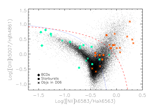
To quantitatively check the analogy between our [OIV] diagram (Figure 1) and the log([NII]/H $\alpha$ ) vs. log([OIII]/H $\beta$ ) diagram used in the optical, we have collected from the literature existing optical data for our starbursts and BCDs. Special care was taken to match the optical apertures to the 11” wide Spitzer IRS-LH slit, in which the [OIV] line is located. This is especially important for the starburst galaxies as many of them are extended. The most appropriate optical datasets for the majority of galaxies were the integrated spectra obtained by Moustakas & Kennicutt (2006) from which we retrieved the optical spectra data for 13 starbursts and 8 BCDs.

To expand our dataset, we also use the data for star-forming galaxies from Dale et al. (2006), which have matchable Spitzer high-resolution mapping spectra extracted with an aperture of 23” $\times$ 15”, and optical spectra taken with an aperture of 20” $\times$ 20”. There are 19 objects with both detections in [OIV]25.89 $\mu$ m and optical lines used in the BPT diagram, which are displayed in the Figure 2 of Dale et al. (2006). In our Figures 3 and 4, we place our samples with optical data, as well as the star-forming galaxies from Dale et al. (2006), in the corresponding optical log([OIII]/H $\beta$ ) vs. log([NII]/H $\alpha$ ) and infrared [OIV]/[SIII] vs. [NeIII]/[NeII] diagrams.The colors of the data symbols in each diagram are assigned by their corresponding classification in the other diagram (see Figure captions). In Figure 4, the galaxies found above Kewley’s line in Figure 3 are red¹¹1We do not have the matching optical data for the AGNs in our sample, but they are expected to lie well to the right of the Kewley’s line., between Kewley’s and Kauffmann’s line are green, and below Kauffmann’s line are blue. We found that most optically identified strong AGNs (marked with red $\times$ ) and starbursts (blue squares) are well separated in the upper and lower branches, especially for values of the [NeIII]/[NeII] ratio greater than $0.3$ . There are four galaxies optically classified as starbursts (blue squares) located in the upper branch in Figure 4. However, we note that their location in the optical diagram in Figure 3 is near the locus where the two branches merge, an area where classification of individual objects is ambiguous.

In the optical diagram of Figure 3, the data points are colored based on their classification in the infrared diagram of Figure 4. More specifically, we empirically define a line separating the upper and lower branch, having the functional form of:

log(\rm{[OIV]/[SIII]})=0.08\times log(\rm{[NeIII]/[NeII]})+0.014

(1)

Galaxies located on the upper branch above the line are plotted in Figure 3 in orange, and below the line in cyan. This demonstrates that the upper and lower branch of the infrared diagram correspond well to the right and left branch of the optical.

We should stress once more that the optical spectra are collected from various sources and have been obtained with different apertures. This likely introduces uncertainties in the separatrix mentioned above, which cannot be easily quantified. Even for datasets where optical and infrared apertures are matched, wavelength dependent extinction will result in discrepancies between the different classifications, in particular for dusty sources, since the infrared can probe into regions which are optically thick. Therefore, it is not surprising to have some outliers that do not correspond to the same regions in both diagrams. For example, galaxies located between Kewley’s and Kauffmann’s line (green objects in Figure 4) may lie either on the upper or lower branch of the infrared diagram. Despite these uncertainties, the overall consistency of the two diagrams is very encouraging, convincing us that the [OIV]/[SIII] vs. [NeIII]/[NeII] diagnostic along with equation (1) can be used to classify the energy source of nuclear emission in galaxies, particularly for those with high dust content.

3.3.2 The [OIV]/[SIII] ratio and other infrared diagnostics

The ratio of the flux of [OIV]25.89 $\mu$ m line with the flux of lower-ionization line has been already proposed to diagnose the dominant source of power in ULIRGs (Genzel et al., 1998; Armus et al., 2007). In the Genzel et al. study, the ratio of [OIV]25.89 $\mu$ m to the [NeII]12.81 $\mu$ m (or [SIII]33.48 $\mu$ m) was plotted against the strength of the 7.7 $\mu$ m PAH. The PAH features are strong in starbursts and weak in AGNs, as the PAH molecules are easily destroyed by the hard radiation of the accretion disk or outshined by the hot dust continuum emission from the AGN torus. In Figure 5, we plot the [OIV]/[SIII] ratio as a function of the equivalent width (EW) of the 6.2 $\mu$ m PAH feature. The PAH EWs for the galaxies in our sample are collected from Brandl et al. (2006); Wu et al. (2006), and Spoon et al. (2007). As was the case with Figure 3 colors of the galaxies in Figure 5 are based on their mid-infrared classification in Figure 4. Those found on the upper branch above the dotted separatrix line are marked in orange, while those on the lower branch are in cyan. We find that the two color groups define two separate trends, with the AGNs residing at the tip of one group and the BCDs at the tip of the other. The upper trend is similar to the trend found in the traditional Genzel et al. diagram (indicated with the upper dashed line), while the other trend clearly falls below it. This suggests that the method to diagnose the fraction of AGN and starburst power in the mid-IR for a given source suggested by Genzel et al. (1998), can only be applied to sources which are part of the upper trend in Figure 5. The upper and lower dashed lines can be represented as equation (2) and (3) respectively:

log(\rm{[OIV]/[SIII]})-log(6.0)=0.19/(log(\rm{EW(6.2)})-log(0.7))

(2)

log(\rm{[OIV]/[SIII]})-log(0.35)=0.51/(log(\rm{EW(6.2)})-log(0.7))

(3)

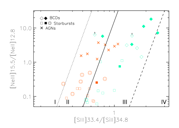
Dale et al. (2006) have also proposed a diagnostic diagram based on the [SIII]33.48 $\mu$ m/[SiII]34.81 $\mu$ m line ratios as a function of the [NeIII]15.56 $\mu$ m/[NeII]12.81 $\mu$ m ratios to distinguish AGN from starburst emission. Their method relies on the fact that [SiII], having an IP of only 8.2 eV, is a low-ionization emission line and a strong coolant of X-ray-irradiated gas (Maloney et al., 1996). AGNs usually have stronger [SiII] emission than starburst galaxies and diagnostic diagrams involving [SiII] present an advantage in cases of faint sources where [OIV] is not easily detected. In Figure 6, we plot the galaxies from our sample on the [SIII]/[SiII] vs [NeIII]/[NeII] diagram, similarly to the Figure 9 of Dale et al. (2006). The galaxies are divided into four regions, and are classified accordingly in a statistical sense: galaxies located in regions I and II should be classified as an AGN with a $1\sigma$ confidence interval of 83%-97% and 73%-88% respectively, and galaxies found in regions III and IV should be classified as a star-forming systems with a $1\sigma$ confidence interval of 84%-93% and 91%-98%, respectively. In Figure 6 , the galaxies are also colored the same way as in Figure 3 and Figure 5. We find that AGNs and star-forming galaxies situated on the upper branch are preferentially located in regions I and II, while BCDs and star forming galaxies on the lower branch are found in regions III and IV. This suggests that the two methods overall agree.

3.4. The nature of the [OIV]25.89 $\mu$ m emission in starbursts

As mentioned in the previous section, the [OIV]25.89 $\mu$ m emission in galaxies cannot originate from the HII regions around main-sequence stars. Instead, it has to be associated either with an AGN component, or with WR stars (Crowther 1999) and/or shock excitation (Lutz et al., 1998). We have already shown in §3.2 and §3.3 that the [OIV] diagram can successfully identify galaxies where an AGN contributes to their mid-IR spectrum as they are placed on the upper branch of the Figure 1. In this section, we present a preliminary analysis on the nature of the [OIV] emission in the starburst galaxies and BCDs of the lower branch, focusing on the interpretation of models which include WR stars and shocks. More detailed study on this subject will be presented in an upcoming paper.

Some of the sources in our sample are classified as Wolf-Rayet galaxies. They show features of WR stars in their optical spectra, most commonly the broad HeII $\lambda 4686\AA$ emission which has an IP of $\sim 54$ eV, similar to [OIV]. Therefore, identifying correlations between WR features and [OIV] emission could, in principle, reveal the contribution of those stars. We cross-matched our BCDs with the WR galaxy catalog presented in Schaerer et al. (1999) and found that seven BCDs (IZw18, SBS0335-052E, UM461, IIZw40, NGC1569, Mrk1450, and NGC1140) as well as two starbursts (NGC1614 and NGC7714) have reported WR features.

Unfortunately, this WR galaxy sample is small, and there are no consistent measurements of the optical WR features from the literature. Thus a direct correlation of the WR strength and the [OIV] line emission could not be established. In Figure 1 we have marked these WR galaxies (Schaerer et al., 1999) as filled symbols. It appears that at least the detections of WR signatures are not closely associated with high [OIV]/[SIII] ratios, instead, they appear to be more correlated with high [NeIII]/[NeII] ratios.

Another way to probe the contribution of the WR stars to the [OIV] emission is by photo-ionization modeling. We perform a tentative exploration of the contribution of those stars to the presence of the O³⁺ ion in our lower branch galaxies with Starburst 99 (Leitherer 1999) and CLOUDY (Ferland 2001). We use Starburst 99 to model the stellar radiation field of an instantaneous burst of star formation aging from 1 to 10 Myrs. All stars have a metallicity of 1/3 Z_⊙ and the follow a Salpeter IMF. The output from Starburst 99 is used as input to CLOUDY in order to estimate the flux of the mid-IR emission lines.

The models predict that the presence of considerable [OIV] emission is directly related to the appearance of the Wolf-Rayet phases, becoming strong around 4 Myrs after the onset of the burst and fading to undetectable levels 2 Myrs later. On the other hand, the [NeIII] line is related to the presence of massive main sequence O stars but also becomes very weak after 6 Myrs. Both [NeII] and [SIII] lines are still strong after 10 Myrs. Consequently the [OIV]/[SIII] and [NeIII]/[NeII] line ratios peak around 4-5 Myrs after the onset of the burst with values of $\sim$ 0.6 and 40 respectively. The value of 0.6 for the [OIV]/[SIII] line ratio agrees with the highest value observed in the galaxies of the lower branch in Figure 1, but the predicted [NeIII]/[NeII] ratio is about a factor of 4 higher than the observed value. Clearly a more systematic study exploring thoroughly the parameter space of the models and comparing them to larger sample of galaxies with mid-IR measurements is required to further investigate this discrepancy.

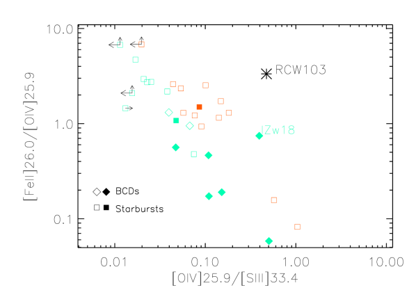
We also study the effects of shocks on the production of [OIV] utilizing infrared lines which are strong in regions of shocks, such as the [FeII]25.99 $\mu$ m (see Lutz et al., 2003). The infrared [FeII] lines have been suggested to trace well of the supernova activity (Greenhouse et al., 1991, see also O’Halloran et al. 2008). The [FeII] ionic abundances in supernova remnants are orders of magnitudes larger than the typical values found in Orion-like HII regions (e.g. Seward et al., 1983; Graham et al., 1987; Oliva et al., 1989). This is primarily due to shock destruction of grains. Since iron is normally depleted onto the grains, the abundance of iron in the ISM is significantly increased in supernova remnants. Furthermore, the cooler and denser gas behind a fast shock generates more low-ionized Fe⁺ compared to what is found in typical HII regions. Following the analysis of Lutz et al. (2003) to evaluate the effects of shocks in NGC6240, we plot in Figure 7 the ratio of [FeII]25.99 $\mu$ m/[OIV]25.89 $\mu$ m as a function of [OIV]25.89 $\mu$ m/[SIII]33.48 $\mu$ m. Also plotted are the measurements of the supernovae remnant RCW103 (Oliva et al., 1999). Most BCDs and starbursts in our sample show an anti-correlation on the diagram, with no obvious indication of enhanced [FeII] emission. However, one galaxy, IZw18, appears to be an outlier compared to other BCDs with a clear enhancement of the [FeII] emission relative to the [OIV] emission. This enhanced [FeII] emission could indicate a significant contribution of shocks in IZw18.

The influence of shocks to the observed [OIV] emission can be better constrained with detailed shock models (e.g. Allen et al., 2008) but we defer this work to a future paper on this topic. Overall, our preliminary study described in this section suggests that there is no strong indication that shocks play an important role in the mid-IR emission of starbursts and BCDs. Hence, WR stars are the most likely culprit of the [OIV] emission seen in the lower-branch galaxies of the Figure 1. We do note though the difficulty to simultaneously fit the [OIV]/[SIII] and [NeIII]/[NeII] ratios with current photo-ionization models. It appears that the models require mechanisms to significantly suppress [NeIII]/[NeII] ratios for a fixed [OIV] emission. This issue is discussed more in §4.

3.5. The [NeV]14.32 $\mu$ m Emission

As we have discussed earlier, BCDs display a significantly harder radiation field than typical starbursts with high [OIV]/[SIII] and [NeIII]/[NeII] ratios. However, no [NeV]14.32 $\mu$ m emission has been detected in any of them. It is known that [NeV], with an IP of 97eV, serves as an unambiguous indicator of an AGN and the 7 out of our 24 starburst galaxies where [NeV]14.32 $\mu$ m was detected, all host an AGN (see table 1 of Bernard-Salas et al., 2009). In Figure 8, we plot the [NeV]14.32 $\mu$ m/[NeII]12.81 $\mu$ m ratio as a function of [NeIII]15.56 $\mu$ m/[NeII]12.81 $\mu$ m for BCDs, starbursts, AGNs, and ULIRGs and find a similar bifurcation signature to the one in Figure 1. This also confirms the bifurcation nature of the [OIV] diagram discussed in §3.2 and §3.3. A similar bifurcation is also seen in the [NeV]14.32 $\mu$ m/[NeII]12.81 $\mu$ m vs. [SIV]10.512 $\mu$ m/[SIII]18.712 $\mu$ m diagram (not plotted).

4. General Excitation of Star Forming Galaxies

In addition to the high-ionization emission lines of [NeV] and [OIV], other common mid-IR emission lines such as [SIV]10.51 $\mu$ m, [SIII]18.71 $\mu$ m, [NeII]12.81 $\mu$ m, and [NeIII]15.56 $\mu$ m have been used in order to probe the ionization field in BCDs and starbursts, the [NeIII]15.56 $\mu$ m/[NeII]12.81 $\mu$ m vs. [SIV]10.51 $\mu$ m/[SIII]18.71 $\mu$ m diagram being such an example (e.g. Verma et al., 2003; Dale et al., 2006; Farrah et al., 2007). Both Wu et al. (2006) and Bernard-Salas et al. (2009) studied this diagram independently for different samples. Here we combine both and also include the data from our comparison sample of AGN, ULIRGs, and HII regions. The study is similar to the one presented by Groves et al. (2008), who also include samples of various galaxy types. The advantage of the present work is that the measurements are more consistent as all data were obtained with the Spitzer high-resolution modules.

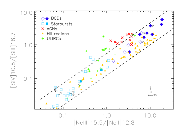
In Figure 9, we plot the [NeIII]15.56 $\mu$ m/[NeII]12.81 $\mu$ m and the [SIV]10.51 $\mu$ m/[SIII]18.71 $\mu$ m ratios for the starbursts, BCDs, AGNs, HII regions, and low-redshift ULIRGs. For the HII regions and the ULIRG sample, only sources with detections in all four lines are displayed. In addition, we include the SH mapping observations of the central positions of NGC5253 (Beirão et al., 2006), a typical BCD with metallicity of 1/6 Z_⊙ (Kobulnicky et al., 1999). Since WR features have also been found in the center of NGC5253, we designate it with a filled diamond as other BCDs with detected WR features.

Observing the plot we note that starbursts populate the lower-left corner of the plot (see also Bernard-Salas et al., 2009). BCDs in general have higher values in both line ratios than the starbursts, while those with WR signatures systematically have even higher [NeIII]/[NeII] and [SIV]/[SIII] ratios than those without. The values of [NeIII]/[NeII] in BCDs reach as high as 20, and [SIV]/[SIII] as high as 10, values which in some cases are even greater than those seen in AGNs. BCDs, starbursts as well as giant HII regions all lie in a band stretching over 3 orders of magnitude in [NeIII]/[NeII] and [SIV]/[SIII]. The band, denoted by the two dashed lines, has a slope of $\sim 0.9$ , similar to the slope obtained by Groves et al. (2008). As discussed by Groves et al. (2008), AGNs and ULIRGs are offset from the band displaying slightly higher [SIV]/[SIII] ratios relative to their [NeIII]/[NeII] ratios. This is very likely due to the harder radiation field in AGNs which excites [SIV] more easily than [NeIII]. However, we notice that the offset is not as significant as in the [OIV] diagram. This indicates that the [NeIII]/[NeII] and [SIV]/[SIII] ratios are not very sensitive to the excitation mechanisms, and cannot be used as diagnostics of the central energy source in a galaxy (Lebouteiller et al., 2008).

The higher [NeIII]/[NeII] and [SIV]/[SIII] ratios in BCDs compared to average starburst galaxies indicate a harder radiation field in BCDs. This had already been well established (e.g. Verma et al., 2003; Dale et al., 2006, and references therein). We note, though, that in our sample of BCDs and starbursts there is little overlap in the values of the [NeIII]/[NeII] and [SIV]/[SIII] ratios with a separatrix at [NeIII]/[NeII] $\sim 1.2$ and [SIV]/[SIII] $\sim 0.4$ . Since our BCDs have preferentially sub-solar metallicities²²2Here we adopt (Ne/H)_⊙=1.2 $\times$ 10^-4 from Feldman & Widing (2003), (S/H)_⊙=1.4 $\times$ 10^-5 from Asplund et al. (2005) and (O/H)_⊙=4.9 $\times$ 10^-4 from Allende Prieto et al. (2001). (Wu et al., 2008a), while the galaxies in the starburst sample are more metal rich (Bernard-Salas et al., 2009), their separation in the diagram suggests that metallicity is likely the dominant parameter determining the [NeIII]/[NeII] and [SIV]/[SIII] ratios.

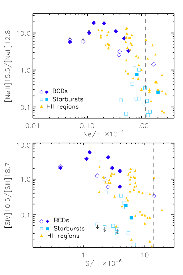
To examine this more directly, we use the metallicity measurements of BCDs, HII regions, and starbursts from Wu et al. (2008a), Lebouteiller et al. (2008), and Bernard-Salas et al. (2009), and plot in Figure 10, the [NeIII]/[NeII] ratios vs. the Ne abundances and [SIV]/[SIII] ratios vs. the S abundances. We observe an anti-correlation between excitation and abundances for both Ne and S, even though there is a substantial scatter (see also Verma et al., 2003; Wu et al., 2006).

As mentioned earlier, the low value of the [NeIII]/[NeII] ratio in starbursts with high metallicities was noted already using ISO data (see also Thornley et al., 2000; Verma et al., 2003; Madden et al., 2006), but its implications are still puzzling. The low ratios apparently suggest a lack of massive stars in the starbursts, in contradiction to the fact that high-mass stars are clearly observed in nearby starbursts (e.g. O’Connell et al., 1995; Whitmore & Schweizer, 1995; Meurer et al., 1995). Thornley et al. (2000) attributed this to an aging effect: massive starbursts have a shorter lifetime, thus, the hottest stars may not be the dominant source of ionization in the starbursts. However, Rigby & Rieke (2004) propose that as high-mass stars spend much of their lives embedded within ultra-compact HII regions (i.e. Charmandaris et al., 2008), the high density and high extinction of the ultra-compact HII regions prevents the mid-infrared nebular lines from forming and escaping.

We note that the starbursts with low [NeIII]/[NeII] ratios have fairly high [OIV]/[SIII] ratios (see Figure 1). This puts additional constraints to the issue of low values of observed [NeIII]/[NeII] ratios. As discussed in §3.4, if WR stars are the main source of the [OIV] emission, the observed values of the [OIV]/[SIII] in starbursts argue strongly against a low mass cutoff of the IMF in these starbursts, since the WR phase would be too short to sustain the intensity of the [OIV] observed. It will also places some constraints on the scenario that massive stars spend much of their life in ultra-compact HII regions. The strong extinction and high density will have to somehow significantly affect [NeIII] and [NeII], but not as much the [OIV] emission.

In Figure 10, we notice that the two extremely low metallicity objects, IZw18 and Tol65 (see Wu et al., 2008b), deviate from the anti-correlation of the emission line ratios vs. the abundances. It appears as if the anti-correlation starts after a maximum value for [NeIII]/[NeII] and [SIV]/[SIII] at $\sim$ 20 and $\sim$ 8 respectively. We should note though that extremely low metallicity galaxies are scarce, and their abundance measurements using the infrared fine-structure lines are more challenging due to the non-detection of their Hu $\alpha$ 12.7 $\mu$ m line. However, similar plots using the oxygen abundance determined from optical spectroscopy also shows the same scatter (Wu et al., 2006).

5. Conclusions

We have presented our analysis of the high spectral resolution mid-IR observations for a sample of 12 BCDs obtained with Spitzer/IRS. A direct comparison with samples of starburst galaxies, AGN, ULIRGs, as well as isolated HII regions, enabled us to extend earlier studies of the ionization and excitation in star forming galaxies towards lower metallicities, and to use the observed mid-IR line emission to explore the excitation mechanisms in these systems.

Although BCDs are known to have a hard radiation field, no [NeV]14.32 $\mu$ m emission has been detected with Spitzer/IRS even for the most metal-poor BCDs.

We find that the [OIV]25.89 $\mu$ m line is commonly detected in the BCDs, starbursts and AGNs. We have demonstrated that the diagram of [OIV]25.89 $\mu$ m/[SIII]33.48 $\mu$ m as a function of [NeIII]15.56 $\mu$ m/[NeII]12.81 $\mu$ m can be useful diagnostic to probe the dominant power source in dust enshrouded systems. Star forming galaxies populate two branches in this diagram, with those harboring an AGN component located on the upper branch, and those without on the lower one. This diagram provides a classification consistent with the log([NII]/H $\alpha$ ) vs. log([OIII]/H $\beta$ ) diagram in the optical, especially for [NeIII]/[NeII] values above 0.3. We empirically define a line (Equation 1) separating galaxies with and without AGN contribution, which could be used in conjunction with other diagnostics to better determine the presence of an AGN in the infrared. A similar bifurcation is seen in a [NeV]/[NeII] vs. [NeIII]/[NeII] diagram. In the [NeIII]/[NeII] vs. [SIV]/[SIII] diagram. AGNs and ULIRGs are only slightly off the band defined by BCDs, starbursts, and HII regions, with higher [SIV]/[SIII] values for given [NeIII]/[NeII] ratios.

In an effort to probe the contribution of shock excitation to the observed [OIV]25.89 $\mu$ m flux, we compare it with the [FeII]25.99 $\mu$ m line , which is a good tracer of supernovae activity. We found no evidence of shock contribution, demonstrated by an enhanced [FeII] emission, in starbursts or BCDs. The only exception is IZw18, which may indicate a significant shock contribution in this low metallicity system.

The most likely contributor to the [OIV] flux, both in starbursts and BCDs, are WR stars. However, current photo-ionization models predict flux ratios of [NeIII]/[NeII] which are too high for the observed [OIV]/[SIII] values. This places an additional constrain on the problem of low [NeIII]/[NeII] ratios already known in high-metallicity starbursts, and will be further investigated in future work.

The authors thank the anonymous referee for useful comments which greatly improved the manuscript. We also thank John Moustakas for kindly providing us the optical data of the SINGS sample. Support for this work was provided by NASA through Contract Number 1257184 issued by the Jet Propulsion Laboratory, California Institute of Technology under NASA contract 1407. V.C. acknowledges partial support from the EU ToK grant 39965 and FP7-REGPOT 206469.

References

Allen et al. (2008) Allen, M. G., Groves, B. A., Dopita, M. A., Sutherland, R. S., & Kewley, L. J. 2008, ApJS, 178, 20
Armus et al. (2007) Armus, L., et al. 2007, ApJ, 656, 148
Baldwin et al. (1981) Baldwin, J. A., Phillips, M. M., & Terlevich, R. 1981, PASP, 93, 5
Beck et al. (2007) Beck, S. C., Turner, J. L., & Kloosterman, J. 2007, AJ, 134, 1237
Beirão et al. (2006) Beirão, P., Brandl, B. R., Devost, D., Smith, J. D., Hao, L., & Houck, J. R. 2006, ApJ, 643, L1
Bernard-Salas et al. (2009) Bernard-Salas, J., et al. 2009, ArXiv e-prints 0908.2812
Brandl et al. (2006) Brandl, B. R., et al. 2006, ApJ, 653, 1129
Brandl et al. (2004) Brandl, B. R., et al. 2004, ApJS, 154, 188
Campbell et al. (1986) Campbell, A., Terlevich, R., & Melnick, J. 1986, MNRAS, 223, 811
Charmandaris et al. (2008) Charmandaris, V., Heydari-Malayeri, M., & Chatzopoulos, E. 2008, A&A, 487, 567
Cohen et al. (2003) Cohen, M., Megeath, S. T., Hammersley, P. L., Martín-Luis, F., & Stauffer, J. 2003, AJ, 125, 2645
Dale et al. (2006) Dale, D. A., et al. 2006, ApJ, 646, 161
Dale et al. (2009) Dale, D. A., et al. 2009, ApJ, 693, 1821
Farrah et al. (2007) Farrah, D., et al. 2007, ApJ, 667, 149
Ferrarese & Merritt (2000) Ferrarese, L., & Merritt, D. 2000, ApJ, 539, L9
Förster Schreiber et al. (2001) Förster Schreiber, N. M., Genzel, R., Lutz, D., Kunze, D., & Sternberg, A. 2001, ApJ, 552, 544
Gebhardt et al. (2000) Gebhardt, K., et al. 2000, ApJ, 539, L13
Genzel et al. (1998) Genzel, R., et al. 1998, ApJ, 498, 579
Gil de Paz et al. (2003) Gil de Paz, A., Madore, B. F., & Pevunova, O. 2003, ApJS, 147, 29
Gorjian et al. (2001) Gorjian, V., Turner, J. L., & Beck, S. C. 2001, ApJ, 554, L29
Graham et al. (1987) Graham, J. R., Wright, G. S., & Longmore, A. J. 1987, ApJ, 313, 847
Greenhouse et al. (1991) Greenhouse, M. A., Woodward, C. E., Thronson, H. A., Jr., Rudy, R. J., Rossano, G. S., Erwin, P., & Puetter, R. C. 1991, ApJ, 383, 164
Groves et al. (2008) Groves, B., Nefs, B., & Brandl, B. 2008, MNRAS, 391, L113
Hao et al. (2005a) Hao, L., et al. 2005a, AJ, 129, 1783
Hao et al. (2005b) Hao, L., et al. 2005b, AJ, 129, 1795
Hao et al. (2007) Hao, L., Weedman, D. W., Spoon, H. W. W., Marshall, J. A., Levenson, N. A., Elitzur, M., & Houck, J. R. 2007, ApJ, 655, L77
Higdon et al. (2004) Higdon, S. J. U., et al. 2004, PASP, 116, 975
Houck et al. (2004a) Houck, J. R., et al. 2004a, ApJS, 154, 18
Houck et al. (2004b) Houck, J. R., et al. 2004b, ApJS, 154, 211
Izotov & Thuan (2008) Izotov, Y. I., & Thuan, T. X. 2008, ApJ, 687, 133
Izotov et al. (2007) Izotov, Y. I., Thuan, T. X., & Guseva, N. G. 2007, ApJ, 671, 1297
Kauffmann et al. (2003) Kauffmann, G., et al. 2003, MNRAS, 346, 1055
Kewley et al. (2001) Kewley, L. J., Dopita, M. A., Sutherland, R. S., Heisler, C. A., & Trevena, J. 2001, ApJ, 556, 121
Kewley et al. (2006) Kewley, L. J., Groves, B., Kauffmann, G., & Heckman, T. 2006, MNRAS, 372, 961
Kobulnicky et al. (1999) Kobulnicky, H. A., Kennicutt, R. C., Jr., & Pizagno, J. L. 1999, ApJ, 514, 544
Laurent et al. (2000) Laurent, O., Mirabel, I. F., Charmandaris, V., Gallais, P., Madden, S. C., Sauvage, M., Vigroux, L., & Cesarsky, C. 2000, A&A, 359, 887
Lebouteiller et al. (2008) Lebouteiller, V., Bernard-Salas, J., Brandl, B., Whelan, D. G., Wu, Y., Charmandaris, V., Devost, D., & Houck, J. R. 2008, ApJ, 680, 398
Li & Draine (2001) Li, A., & Draine, B. T. 2001, ApJ, 554, 778
Lutz et al. (1998) Lutz, D., Kunze, D., Spoon, H. W. W., & Thornley, M. D. 1998, A&A, 333, L75
Lutz et al. (2003) Lutz, D., Sturm, E., Genzel, R., Spoon, H. W. W., Moorwood, A. F. M., Netzer, H., & Sternberg, A. 2003, A&A, 409, 867
Madden et al. (2006) Madden, S. C., Galliano, F., Jones, A. P., & Sauvage, M. 2006, A&A, 446, 877
Magorrian et al. (1998) Magorrian, J., et al. 1998, AJ, 115, 2285
Maloney et al. (1996) Maloney, P. R., Hollenbach, D. J., & Tielens, A. G. G. M. 1996, ApJ, 466, 561
Meurer et al. (1995) Meurer, G. R., Heckman, T. M., Leitherer, C., Kinney, A., Robert, C., & Garnett, D. R. 1995, AJ, 110, 2665
Moustakas & Kennicutt (2006) Moustakas, J., & Kennicutt, R. C., Jr. 2006, ApJS, 164, 81
Nardini et al. (2008) Nardini, E., Risaliti, G., Salvati, M., Sani, E., Imanishi, M., Marconi, A., & Maiolino, R. 2008, MNRAS, 385, L130
O’Connell et al. (1995) O’Connell, R. W., Gallagher, J. S., III, Hunter, D. A., & Colley, W. N. 1995, ApJ, 446, L1
O’Halloran et al. (2008) O’Halloran, B., Madden, S. C., & Abel, N. P. 2008, ApJ, 681, 1205
Oliva et al. (1989) Oliva, E., Moorwood, A. F. M., & Danziger, I. J. 1989, A&A, 214, 307
Oliva et al. (1999) Oliva, E., Moorwood, A. F. M., Drapatz, S., Lutz, D., & Sturm, E. 1999, A&A, 343, 943
Peeters et al. (2002) Peeters, E., et al. 2002, A&A, 381, 571
Rigby & Rieke (2004) Rigby, J. R., & Rieke, G. H. 2004, ApJ, 606, 237
Schaerer et al. (1999) Schaerer, D., Contini, T., & Pindao, M. 1999, A&AS, 136, 35
Schaerer & Stasińska (1999) Schaerer, D., & Stasińska, G. 1999, A&A, 345, L17
Seward et al. (1983) Seward, F. D., Harnden, F. R., Jr., Murdin, P., & Clark, D. H. 1983, ApJ, 267, 698
Spoon et al. (2007) Spoon, H. W. W., Marshall, J. A., Houck, J. R., Elitzur, M., Hao, L., Armus, L., Brandl, B. R., & Charmandaris, V. 2007, ApJ, 654, L49
Thornley et al. (2000) Thornley, M. D., Schreiber, N. M. F., Lutz, D., Genzel, R., Spoon, H. W. W., Kunze, D., & Sternberg, A. 2000, ApJ, 539, 641
Thuan & Martin (1981) Thuan, T. X., & Martin, G. E. 1981, ApJ, 247, 823
Vacca et al. (2002) Vacca, W. D., Johnson, K. E., & Conti, P. S. 2002, AJ, 123, 772
Veilleux & Osterbrock (1987) Veilleux, S., & Osterbrock, D. E. 1987, ApJS, 63, 295
Verma et al. (2005) Verma, A., Charmandaris, V., Klaas, U., Lutz, D., & Haas, M. 2005, Space Science Reviews, 119, 355
Verma et al. (2003) Verma, A., Lutz, D., Sturm, E., Sternberg, A., Genzel, R., & Vacca, W. 2003, A&A, 403, 829
Wehner et al. (2006) Wehner, E. H., Gallagher, J. S., Papaderos, P., Fritze-von Alvensleben, U., & Westfall, K. B. 2006, MNRAS, 371, 1047
Werner et al. (2004) Werner, M. W., et al. 2004, ApJS, 154, 1
Whitmore & Schweizer (1995) Whitmore, B. C., & Schweizer, F. 1995, AJ, 109, 960
Wu et al. (2008a) Wu, Y., Bernard-Salas, J., Charmandaris, V., Lebouteiller, V., Hao, L., Brandl, B. R., & Houck, J. R. 2008a, ApJ, 673, 193
Wu et al. (2008b) Wu, Y., Charmandaris, V., Houck, J. R., Bernard-Salas, J., Lebouteiller, V., Brandl, B. R., & Farrah, D. 2008b, ApJ, 676, 970
Wu et al. (2006) Wu, Y., Charmandaris, V., Hao, L., Brandl, B. R., Bernard-Salas, J., Spoon, H. W. W., & Houck, J. R. 2006, ApJ, 639, 157

Table 1Mid-Infrared Line Measurements of BCDs

	Flux^a^aThe integrated fluxes are measured from the high resolution spectra of the targets. Background emission has not been subtracted and no scaling between the SH and LH modules of IRS has been applied. The central wavelength and the ionization potential of each line are indicated. ( $\times 10^{-16}$ W m^-2)
Object Name	[SIV]	[NeII]	[NeIII]	[SIII]	[SIII]	[SiII]	[NeV]	[NeV]	[OIV]	[FeII]
	10.51 $\mu$ m	12.81 $\mu$ m	15.56 $\mu$ m	18.71 $\mu$ m	33.48 $\mu$ m	34.81 $\mu$ m	14.32 $\mu$ m	24.32 $\mu$ m	25.89 $\mu$ m	25.99 $\mu$ m
	34.8eV	21.6eV	41.0eV	23.3eV	23.3eV	8.2eV	97.1eV	97.1eV	54.9eV	7.9eV
Haro11	4.396 $\pm$ 0.030	3.114 $\pm$ 0.027	9.801 $\pm$ 0.058	4.523 $\pm$ 0.041	6.773 $\pm$ 0.351	5.165 $\pm$ 0.267	$<$ 0.076	$<$ 0.554	0.456 $\pm$ 0.116	0.433 $\pm$ 0.188
NGC1140	1.226 $\pm$ 0.014	1.138 $\pm$ 0.025	3.770 $\pm$ 0.032	2.007 $\pm$ 0.013	4.071 $\pm$ 0.078	2.777 $\pm$ 0.088	$<$ 0.015	$<$ 0.081	0.192 $\pm$ 0.037	0.108 $\pm$ 0.044
SBS0335-052E	0.155 $\pm$ 0.004	$<$ 0.014	0.142 $\pm$ 0.005	0.042 $\pm$ 0.009	0.204 $\pm$ 0.027	$<$ 0.150	$<$ 0.012	$<$ 0.042	0.103 $\pm$ 0.018	0.006 $\pm$ 0.007
NGC1569	14.764 $\pm$ 0.080	1.576 $\pm$ 0.030	17.583 $\pm$ 0.095	7.270 $\pm$ 0.055	19.197 $\pm$ 0.468	10.113 $\pm$ 0.444	$<$ 0.069	$<$ 0.460	2.917 $\pm$ 0.223	0.554 $\pm$ 0.124
IIZw40	18.555 $\pm$ 0.141	0.622 $\pm$ 0.024	11.299 $\pm$ 0.085	4.581 $\pm$ 0.045	8.199 $\pm$ 0.156	3.672 $\pm$ 0.215	$<$ 0.054	$<$ 0.286	0.899 $\pm$ 0.119	0.155 $\pm$ 0.066
UGC4274	0.422 $\pm$ 0.016	0.898 $\pm$ 0.028	1.281 $\pm$ 0.030	1.265 $\pm$ 0.033	3.008 $\pm$ 0.156	1.661 $\pm$ 0.124	$<$ 0.044	$<$ 0.100	0.119 $\pm$ 0.032	0.156 $\pm$ 0.037
IZw18	0.045 $\pm$ 0.007	0.008 $\pm$ 0.002	0.046 $\pm$ 0.005	0.022 $\pm$ 0.005	0.109 $\pm$ 0.024	0.141 $\pm$ 0.049	$<$ 0.010	$<$ 0.035	0.043 $\pm$ 0.008	0.032 $\pm$ 0.010
VIIZw403	0.107 $\pm$ 0.013	$<$ 0.015	0.089 $\pm$ 0.006	0.087 $\pm$ 0.007	0.159 $\pm$ 0.074	0.108 $\pm$ 0.038	$<$ 0.015	$<$ 0.040	$<$ 0.030	$<$ 0.030
Mrk1450	0.734 $\pm$ 0.010	0.134 $\pm$ 0.007	0.963 $\pm$ 0.008	0.438 $\pm$ 0.010	0.774 $\pm$ 0.157	0.300 $\pm$ 0.107	$<$ 0.011	$<$ 0.040	0.084 $\pm$ 0.011	0.039 $\pm$ 0.010
UM461	0.456 $\pm$ 0.009	0.015 $\pm$ 0.005	0.281 $\pm$ 0.008	0.081 $\pm$ 0.006	$<$ 0.153	0.091 $\pm$ 0.018	$<$ 0.015	$<$ 0.064	$<$ 0.045	$<$ 0.045
Tol65	0.069 $\pm$ 0.007	$<$ 0.014	0.089 $\pm$ 0.005	0.031 $\pm$ 0.006	0.129 $\pm$ 0.037	0.198 $\pm$ 0.037	$<$ 0.009	$<$ 0.024	$<$ 0.028	$<$ 0.028
Mrk1499	0.175 $\pm$ 0.006	0.194 $\pm$ 0.009	0.502 $\pm$ 0.006	0.291 $\pm$ 0.005	0.616 $\pm$ 0.039	0.375 $\pm$ 0.046	$<$ 0.009	$<$ 0.025	$<$ 0.028	$<$ 0.028