Good shadows, dynamics, and convex hulls

Abstract. The Ekeland variational principle implies what can be regarded as a strong version, in the $C^{1}$ category, of the Yau minimum principle: under the appropriate hypotheses every minimizing sequence admits a good shadow, a second minimizing sequence that has good properties and is asymptotic to the original one. Using arguments from dynamical systems, we give another proof of this result and also establish, with the aid of Gromov’s theorem on monotonicity of volume ratios, a special case of a conjecture claiming the existence of good shadows in the original $C^{2}$ setting of the Yau minimum principle. The interest in having an abundance of good shadows stems from the fact that this is a desirable property if one wants to refine the applications of the asymptotic minimum principle, as it allows for information to be localized at infinity. These ideas are applied in this paper to the study of the convex hulls of complete submanifolds of Euclidean $n$-space that have controlled Grassmanian-valued Gauss maps.

1 Introduction

The well known Yau minimum principle ([3],[12],[18]), stated below, is a powerful tool in geometric analysis (see, for instance, [8],[14],[19]):

Theorem 1.1.

Let $M$ be a complete manifold whose Ricci curvature is bounded from below, and $f:M\to\mathbb{R}$ of class $C^{2}$ such that $\inf_{M}f>-\infty$. Then, there exists a sequence $(x_{n})$ in $M$ satisfying $f(x_{n})\to\inf_{M}f$, $||\nabla f(x_{n})||\to 0$ and $\liminf_{n\to\infty}\Delta f(x_{n})\geq 0$.

By analogy, one may ask the following question: If $f$ is supposed to be only of class $C^{1}$, is there a minimizing sequence for $f$ along which the gradient of $f$ is small? In the following theorem we observe not only that such special sequences exist, but also that they can be found asymptotically near any specified minimizing sequence.

Theorem 1.2.

Let $M$ be a complete manifold, and $f:M\to\mathbb{R}$ of class $C^{1}$ such that $\inf_{M}f>-\infty$. Then, for every sequence $(x_{n})$ in $M$ such that $f(x_{n})\to\inf_{M}f$, there exists a sequence $(y_{n})$ in $M$ such that $d(x_{n},y_{n})\to 0$, $f(y_{n})\to\inf_{M}f$ and $||\nabla f(y_{n})||\to 0$.

As we will see, this abundance of “good”minimizing sequences will allow us to establish a sharp geometric application that does not follow from the Yau minimum principle, even in the $C^{\infty}$ case (Theorem 1.4).

The formal similarity between Theorems 1.1 and 1.2 is manifest, except for the statement about special minimizing sequences that are asymptotically close to an arbitrary minimizing one.

Definition. Let $M$ be a complete non-compact Riemannian manifold, and $f:M\to\mathbb{R}$ a function of class $C^{2}$ satisfying $\inf f>-\infty$. A minimizing sequence $(p_{n})$ of $f$ is said to admit a good shadow if there exists a minimizing sequence $(q_{n})$ in $M$ such that $\lim d(p_{n},q_{n})=0$,  $\lim||\nabla f(q_{n})||=0$,  and  $\liminf\Delta f(q_{n})\geq 0$ (likewise, if $f$ is $C^{1}$ one only requires the first two properties).

The analogy between the two theorems above will be complete if the following can be shown to be true:

Conjecture.  Let $f:M\to\mathbb{R}$ be of class $C^{2}$, $\inf f>-\infty$, $M$ a complete manifold with Ricci curvature bounded below. Then every minimizing sequence of $f$ has a good shadow.

In $\S 2$ we offer two proofs of Theorem 1.2. The first one is based on the Ekeland variational principle ([5], [6], [15]), a well known result in control theory and non-linear analysis. A new line of argument, based on ideas from dynamical systems, is also presented. The reason for including the second proof here is that a considerable elaboration of it, together with a result of Gromov, yields the following special case of the good shadows conjecture (see also Theorem 3.1):

Theorem 1.3.

Let $M^{m}$ be a complete manifold with Ricci curvature bounded from below, and $f:M\to\mathbb{R}$ a function of class $C^{2}$ such that $\inf f>-\infty$ and $\sup||Hessf||<\infty$. Then every minimizing sequence of $f$ admits a good shadow.

A compelling reason for examining the above conjecture – one that goes beyond a mere comparison between the Ekeland variational principle and the Yau minimum principle – is that the good shadow property is a useful tool to have if one wants to refine the applications of the asymptotic minimum principle, as it allows for information to be localized at infinity. Indeed, this is the philosophy behind the proofs of Theorems 1.4 and 1.7 below.

The remarks of the last paragraph are best understood in the applications of the asymptotic minimum (maximum) principle to the study of submanifolds. In these problems, geometric intuition can often help to locate in space a particular (but, a priori, not sufficiently well-behaved) minimizing sequence. One can then try to find a good shadow of this sequence, for which the computations of the relevant quantities can yield the desired result.

In what follows we describe how the ideas outlined above can be used, in the context of Theorem 1.2, to study the problem of characterizing the convex hulls of $C^{1}$ immersed submanifolds that have controlled Gauss maps.

Due to the low regularity, the usual tools of submanifold geometry, centered as they are on the study of the second fundamental form, cannot be applied to $C^{1}$ submanifolds. Nevertheless, these are naturally occurring objects, worthy of study. For instance, it follows from a theorem of Nash-Kuiper [9] that every Riemannian manifold $M^{m}$ admits an isometric $C^{1}$-embedding into an arbitrarily small neighborhood of $R^{2m}$. Of course, for smoother immersions the expected codimension is much higher [7]. See also the end of this Introduction for an interesting question regarding $C^{1}$ isometric immersions, in the context of the present paper.

Any non-empty open convex subset $\cal O$ of $\mathbb{R}^{n}$ is the convex hull of a $C^{\infty}$ complete submanifold, of any codimension. To see this when $n\geq 3$, take a smooth curve $\Gamma\subset\cal O$, of infinite length on both ends, whose convex hull is $\cal O$. Let $M$ be the union over all $p\in\Gamma$ of smoothly varying $k$-dimensional spheres $S^{(k)}_{r(p)}$, $1\leq k\leq n-2$, centered at $p$ and contained in the normal space of $\Gamma$ at $p$. Taking $r(p)$ to decay fast enough one can make sure that the resulting manifold $M$, which is automatically complete, is contained in $\cal O$. Since $p$ is in the convex hull of $S^{(k)}_{r(p)}$ for any $p\in\Gamma$, it follows that the convex hull of $M$ satisfies $\text{Conv}\,(M)=\cal O$.

Using Theorem 1.2, we show that there are obstructions for a given convex set to be the convex hull of a complete $C^{1}$ submanifold of a fixed codimension, provided the Gauss map, which is of course continuous, is assumed to be uniformly continuous.

Recall that $h:M^{m}\to\mathbb{R}^{n}$ is said to be substantial if $h(M)$ is not contained in a proper affine subspace of $\mathbb{R}^{n}$.

Theorem 1.4.

Let $M$ be a complete $m$-dimensional Riemannian manifold, $n>m$, and $h:M\to\mathbb{R}^{n}$ a substantial $C^{1}$ isometric immersion for which the Grassmanian-valued Gauss map $\mathcal{G}:M\to G(n-m,n)$, given by $\mathcal{G}(p)=[h_{\ast}TM_{p}]^{\perp}$, is uniformly continuous. Then either $\text{Conv}\,[h(M)]=\mathbb{R}^{n}$, or each point in the boundary of $\text{Conv}\,[h(M)]$ admits at most $n-m$ supporting hyperplanes in general position.

Corollary 1.5.

If $h:M^{m}\to\mathbb{R}^{n}$ is a substantial $C^{1}$ immersion of a compact manifold, then each point in the boundary of $\text{Conv}\,[h(M^{m})]$ admits at most $n-m$ supporting hyperplanes in general position.

Observing that the limit of supporting hyperplanes is itself a supporting hyperplane, we have:

Corollary 1.6.

If $M^{n-1}$ is compact and $h:M^{n-1}\to\mathbb{R}^{n}$ is a $C^{1}$ immersion, then $h$ is substantial and each point $p$ in the boundary of $\text{Conv}\,[h(M^{n-1})]$ admits a unique support hyperplane $H_{p}$. Moreover, the map $p\mapsto H_{p}$ is continuous.

Theorem 1.3 also has applications to the geometry of submanifolds:

Theorem 1.7.

Let $M^{m}$ be a complete manifold, $n>m$, and $h:M^{m}\to\mathbb{R}^{n}$ a substantial $C^{2}$ isometric immersion, with bounded second fundamental form and uniformly continuous mean curvature vector field $\overrightarrow{H}$. Suppose $\text{Conv}\,[h(M^{m})]\neq\mathbb{R}^{n}$ and let $H_{1},\ldots,H_{s}$ be supporting hyperplanes in general position that pass through a point $p_{o}$ of the boundary of $\text{Conv}\,[h(M^{m})]$. Let $e_{i}\in[H_{i}]^{\perp}$ be the unit vector such that $\langle h(x)-p_{o},e_{i}\rangle\geq 0$ for every $x\in M^{m},\;i=1,...,s$. Then $s\leq n-m$ and there exists a sequence $(p_{k})$ in $M^{m}$ such that $\text{d}(h(p_{k}),H_{1}\cap\dots\cap H_{s})\to 0$ and $\liminf_{k\to\infty}\left\langle\overrightarrow{H}(p_{k}),e_{i}\right\rangle\geq 0,\;i=1,\ldots,s$.

The following result can be viewed as a generalization of the fact that the mean curvature of a compact convex hypersurface of $\mathbb{R}^{n}$ is nonnegative, after an appropriate choice of the orientation.

Theorem 1.8.

Let $h:M^{m}\to\mathbb{R}^{n}$ be a substantial $C^{2}$ isometric immersion of a compact Riemannian manifold $M^{m}$, and $H_{1},\ldots,H_{s}$ supporting hyperplanes in general position that pass through a point $p_{o}$ of the boundary of $\text{Conv}\,[h(M^{m})]$. Let $e_{1},\ldots,e_{s}$ be as in the statement of the Theorem 1.7. Then $s\leq n-m$, $h(M)\cap H_{1}\cap\dots\cap H_{s}\neq\emptyset$, and for every point $q\in M^{n}$ such that $h(q)\in H_{1}\cap\dots\cap H_{s}$ one has $\left\langle\overrightarrow{H}(q),e_{i}\right\rangle\geq 0,\;i=1,\ldots,s$.

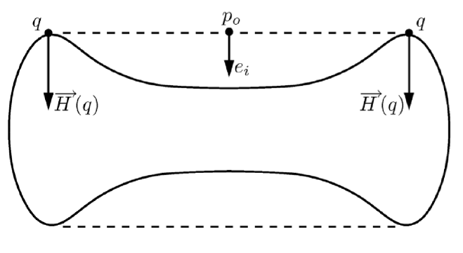
Fig. 1: Theorem 1.8

Examples. It is easy to illustrate Theorem 1.4, already in low dimensions:

i) Let $l$ be a line in $\mathbb{R}^{3}$, and $P_{1}$, $P_{2}$ planes such that $P_{1}\cap P_{2}=l$. Let $\cal O$ be a component of $\mathbb{R}^{3}-(P_{1}\cup P_{2})$. One can construct a complete $C^{\infty}$ curve $\Gamma\subset\cal O$ such that $\text{Conv}\;(\Gamma)=\cal O$ and $\Gamma$ has bounded curvature. The last condition ensures that the Gauss map $\mathcal{G}:\Gamma\to G(2,3)$ is uniformly continuous. Along $l$, the maximum number of supporting hyperplanes to $\partial\cal O$ that are in general position is two, which is also the codimension of $\Gamma$. This gives the equality case in Theorem 1.4.

We give an informal description of how $\Gamma$ can be constructed. Start with oriented line segments $l_{n}$ parallel to $l$, $n\geq 1$, contained in $\cal O$, getting longer as $n\to\infty$, and accumulating onto the entire oriented line $l$. One obtains $\Gamma$ by connecting for all $n\geq 1$ the last point of $l_{n}$, in a smooth way, to the first point of $l_{n+1}$, by means of a curve $\gamma_{n}$ of curvature less than one. The curve $\gamma_{n}$ is supposed to be very long, going deep inside $\cal O$ and turning slowly, so that the curvature can be kept smaller than one. Once $\gamma_{n}$ is far from $l$, one can also make $\gamma_{n}$ twist around, with controlled curvature, so as to make its convex hull bigger. It is now clear that a sequence of curves $\gamma_{n}$ can be created so that $\Gamma$ has curvature less than one and $\text{Conv}\;(\Gamma)=\cal O$.

Observe that such a construction is impossible if, instead of a curve, one takes $\Gamma$ to be a complete surface. Indeed, as the surface gets closer and closer to $l$, in order for $\Gamma$ to remain in $\cal O$ it has to fold abruptly, thus violating the condition that the Gauss map is uniformly continuous.

ii) Let $M$ be an open hemisphere in $S^{2}\subset\mathbb{R}^{3}$. Its convex hull is, of course, the solid hemisphere. At points along the great circle, $\text{Conv}\;(M)$ has two supporting hyperplanes in general position, whereas the codimension of $M$ is one. This shows that Theorem 1.4 fails if the submanifold is not complete.∎

The uniform continuity condition on the Gauss map allows for the Ricci curvature of the submanifold to be unbounded from below. In fact, it is easy to construct smooth complete graphs in $\mathbb{R}^{3}$ with these properties. This shows that Theorem 1.1 cannot be applied to prove Theorem 1.4, even if the submanifold in question is of class $C^{\infty}$.

To put these remarks in perspective note that, by the Gauss equation, the natural way to force the intrinsic curvatures of a submanifold to be bounded is simply to require that the second fundamental form has bounded length. Although this is not obvious, at least in the case of hypersurfaces the latter condition means that the Gauss map is globally Lipschitzian, which is stronger than merely requiring the Gauss map to be uniformly continuous.

We stress that, in Theorem 1.4, even if the submanifold is $C^{\infty}$ and has bounded second fundamental form, the Yau minimum principle cannot be applied. Indeed, as it will be clear from the proof, one needs to find good shadows that are provided in the $C^{1}$ context by Theorem 1.2, for arbitrary minimizing sequences. Theorem 1.1, on the other hand, guarantees the existence of a single minimizing sequence with “good”properties.

A natural question is whether the condition in Theorem 1.4, stating that the boundary points of the convex hull admits at most $n-m$ tangent hyperplanes in general position, is also sufficient for the construction of examples. Here, again, one ought to keep in mind that the Gauss map is only required to be uniformly continuous, instead of the stronger condition of being Lipschitz. We are indebted to J. Fu for pointing out that the work of Alberti [1] may be relevant to this question.

Another interesting problem concerning immersions with uniformly continuous Gauss maps, albeit unrelated to the actual results in the present paper, has to do with the isometric immersions $\varphi:M^{2}\to R^{3}$ of Hadamard surfaces with curvature bounded away from zero. By Efimov’s theorem [4], no such $\varphi$ exists that is of class $C^{2}$. On the other hand, by the Nash-Kuiper’s theorem [9] there is a $\varphi$ of class $C^{1}$; in particular, its Gauss map is continuous. If $M^{2}$ is as above, does there exist a $C^{1}$ isometric immersion $\varphi:M^{2}\to\mathbb{R}^{3}$ whose Gauss map is uniformly continuous? By [9], the answer is yes if $M^{2}$ is the universal cover of a compact surface with negative curvature.

Finally, we refer to [16] for other geometric properties that can be recovered from Grassmanian-valued Gauss maps.

2 A strong $\bf C^{1}$ version of the Yau minimum principle

For the first proof of Theorem 1.2 we will need the following fundamental result ([5], [6], [15]):

The Ekeland Variational Principle. Let $(X,d)$ be a complete metric space, and $f:X\to\mathbb{R}$ a function which is lower semi-continuous and bounded from below. Then for any $\varepsilon,\delta>0$, and $x\in X$ with $f(x)\leq\inf_{X}f+\varepsilon$, there is $y\in X$ satisfying

i) $d(x,y)\leq\delta$

ii) $f(y)\leq f(x)$

iii) $f(y)<f(z)+\frac{\varepsilon}{\delta}d(y,z)$,   for all $z\in X$ with $z\neq y$.

First proof of Theorem 1.2. For each $n\in\mathbb{N}$, let $\varepsilon_{n}=f(x_{n})-\inf_{M}f$, $\delta_{n}=\sqrt{\varepsilon_{n}}$. In the sequel we will prove the existence of a sequence $(y_{n})$ in $M$ satisfying

$$f(y_{n})\leq f(x_{n}),\;\;\;d(x_{n},y_{n})\leq\delta_{n}$$ (2.1)

and

$$||\nabla f||(y_{n})\leq\delta_{n}.$$ (2.2)

Since $\delta_{n}\to 0$ as $n\to\infty$, $(y_{n})$ will have the desired properties. If $f(x_{n})=\inf_{M}f$, take $y_{n}=x_{n}$. Otherwise, we have $\varepsilon_{n}>0$, $\delta_{n}>0$, and applying the Ekeland Variational Principle with $\varepsilon=\varepsilon_{n}$, $\delta=\delta_{n}$ and $x=x_{n}$, we obtain $y_{n}\in M$ satisfying (2.1) and

$$f(y_{n})<f(z)+\frac{\varepsilon_{n}}{\delta_{n}}d(y_{n},z)=f(z)+\delta_{n}\,d(y_{n},z),$$ (2.3)

for all $z\in M$ with $z\neq y_{n}$. To show (2.2), take an arbitrary unit vector $v\in T_{y_{n}}M$ and let $\gamma:(-c,c)\to M$ be the unit speed geodesic in $M$ so that $\gamma(0)=y_{n}$ and $\gamma^{\prime}(0)=v$. Reducing $c$ if necessary, we can suppose that the image of $\gamma$ is contained in a normal neighborhood of $y_{n}$ in M. From (2.3) we have, with $z=\gamma(t)$,

$$f\big{(}\gamma(t)\big{)}-f(y_{n})>-\delta_{n}\,d\big{(}\gamma(t),y_{n}\big{)}=-\delta_{n}\,|t|,\;\;\;0<|t|<c,$$ (2.4)

which implies

$$\frac{f\big{(}\gamma(t)\big{)}-f(y_{n})}{t}<\delta_{n},\;\;\;-c<t<0.$$ (2.5)

Since $f$ is of class $C^{1}$, it follows that

$$\langle\nabla f(y_{n}),v\rangle=\frac{d}{dt}\Big{|}_{t=0}f\circ\gamma(t)=\lim_{t\to 0^{-}}\frac{f\big{(}\gamma(t)\big{)}-f(y_{n})}{t}\leq\delta_{n},$$ (2.6)

for all $v\in T_{y_{n}}M$ with $||v||=1$. Therefore,

$$\big{|}\langle\nabla f(y_{n}),v\rangle\big{|}\leq\delta_{n},$$ (2.7)

for all unit vector $v\in T_{y_{n}}M$, so that

$$||\nabla f(y_{n})||\leq\delta_{n},\;\;\;n\in\mathbb{N}.$$ (2.8)

The sequence $(y_{n})$ satisfies (2.1) and (2.2) and thus the conditions of the theorem. ∎

Second proof of Theorem 1.2. For each $n\in\mathbb{N}$, let

$$r_{n}=\sqrt{f(x_{n})-\inf_{M}f}.$$ (2.9)

As in the first proof of Theorem 1.2, we will construct a sequence $(y_{n})$ in $M$ satisfying

$$f(y_{n})\leq f(x_{n}),\;\;\;d(x_{n},y_{n})\leq r_{n},\;\;\;||\nabla f||(y_{n})\leq r_{n},$$ (2.10)

for all $n\in\mathbb{N}$. The conclusion that $(y_{n})$ meets the conditions of the theorem will follow from the fact that $r_{n}\to 0$ when $n\to\infty$. If $\nabla f(x_{n})=0$, take $y_{n}=x_{n}$. In case $\nabla f(x_{n})\neq 0$, denote by $\gamma_{n}:[0,\tau_{n})\to M$ the maximal integral curve of the vector field $X=-||\nabla f||^{-2}\,\nabla f$ such that $\gamma_{n}(0)=x_{n}$. From $(f\circ\gamma_{n})^{\prime}=-1$, we obtain

$$f(\gamma_{n}(t))-f(x_{n})=-t$$ (2.11)

for all $t$ in $[0,\tau_{n})$. Recall that $q\in M$ belongs to the $w$-limit set of $\gamma_{n}$ if there exists a sequence $(t_{k})$ contained in $[0,\tau_{n})$ such that $\lim_{k\to\infty}t_{k}=\tau_{n}$ and $\lim_{k\to\infty}\gamma_{n}(t_{k})=q$. The orbits of X are also orbits of $-\nabla f$. It follows from ([13], p. 13) that the $w$-limit set of $\gamma_{n}$ consists entirely of critical points of $f$. Denote by $\overline{B}(x_{n},r_{n})$ the closed ball with center at $x_{n}$ and radius $r_{n}$. We have two cases to consider:

i) The $\omega$-limit set of $\gamma_{n}$ contains a point $q_{n}$ in $\overline{B}(x_{n},r_{n})$. As observed above, $q_{n}$ is necessarily a critical point for $f$ and we set $y_{n}=q_{n}$.

ii) The $\omega$-limit set of $\gamma_{n}$ does not intersect $\overline{B}(x_{n},r_{n})$. Let $t_{n}$ be the first time such that the positive trajectory of $X$ through $x_{n}$ hits $\partial B(x_{n},r_{n})$. We have

$$r_{n}\leq\hbox{length}\;\gamma_{n}|_{[0,t_{n}]}=\int_{0}^{t_{n}}||\gamma_{n}^{\prime}(t)||dt\leq t_{n}\;\max_{\gamma_{n}|_{[0,t_{n}]}}(||\nabla f||^{-1}),$$ (2.12)

so that, by (2.11),

$$r_{n}\min_{\gamma_{n}|_{[0,t_{n}]}}||\nabla f||\leq t_{n}=f(x_{n})-f(\gamma_{n}(t_{n}))<f(x_{n})-\inf_{M}f.$$ (2.13)

It follows from (2.9) and (2.13) that

$$\min_{\gamma_{n}|_{[0,t_{n}]}}||\nabla f||<r_{n}.$$ (2.14)

Choosing $\theta_{n}\in[0,t_{n}]$ so that $||\nabla f||(\gamma_{n}(\theta_{n}))=\min_{\gamma_{n}|_{[0,t_{n}]}}||\nabla f||$ and taking $y_{n}=\gamma_{n}(\theta_{n})$, we have $f(y_{n})\leq f(x_{n})$ and, since $\gamma_{n}([0,t_{n}])\subset\overline{B}(x_{n},r_{n})$,

$$d(x_{n},y_{n})\leq r_{n}=\sqrt{f(x_{n})-\inf_{M}f}.$$

Moreover, by (2.14), $||\nabla f||(y_{n})<r_{n}$. Hence the sequence $(y_{n})$ satisfies (2.10) and thus the conditions of the theorem.∎

3 Flows and asymptotic minimum principles

In this section we study the conjecture from the Introduction, using gradient flows as in the second proof of Theorem (1.2). Here, however, the situation is much more complex and only partial results are available. Instead of estimating only lengths, one needs to estimate both lengths and volumes. Further refinements of the basic strategy may yet yield a proof of the full conjecture.

Proof of Theorem 1.3. Let $\phi_{t}$ be the local flow of $X=-\nabla f$ on $M$, so that

$$\frac{d}{dt}\phi_{t}(p)=-\nabla f(\phi_{t}(p)),\;\;\phi_{0}(p)=p,$$ (3.1)

where $t\in[0,\tau(p))=$ the maximal interval of existence of the forward solution.

For each $n\in\mathbb{N}$, set

$$\delta_{n}=\sqrt{f(p_{n})-\inf_{M}f},\;\;\;r_{n}=\sqrt{\delta_{n}}.$$ (3.2)

Since $\delta_{n}\to 0$ as $n\to\infty$, we may suppose, without loss of generality, that $\delta_{n}<r_{n}$ for all $n\in\mathbb{N}$. We will construct a sequence $(q_{n})$ in $M$ satisfying

$$\text{d}(p_{n},q_{n})\leq r_{n},\;\;\;\liminf_{n\to\infty}\Delta f(q_{n})\geq 0.$$ (3.3)

If $\delta_{n}=0$, we have $\Delta f(p_{n})\geq 0$ and we choose $q_{n}=p_{n}$. Fix $n\in\mathbb{N}$ so that $\delta_{n}>0$. We are going to distinguish between two cases:

a) Every positive orbit originating in $\overline{B}(p_{n},r_{n}^{2})$ remains in the open ball $B(p_{n},r_{n})$.

b) There is at least one trajectory that joins the boundaries of $B(p_{n},r_{n}^{2})$ and $B(p_{n},r_{n})$ in finite time.

In the first alternative, $\tau(p)=\infty$ for every $p\in\overline{B}(p_{n},r_{n}^{2})$. Let $\mu$ denote the Riemannian measure of $M$. By Liouville’s formula for the change of volume under a flow [10], one has, for all $t>0$, since $\Delta=\text{div}\nabla$,

$$\mu\big{(}B(p_{n},r_{n})\big{)}\geq\mu\big{(}\phi_{t}(B(p_{n},r_{n}^{2}))\big{)}=\int_{B(p_{n},r_{n}^{2})}\exp\Big{(}\int_{0}^{t}-\Delta f(\phi_{s}(p))ds\Big{)}d\mu(p).$$ (3.4)

If there exists $\varepsilon>0$ such that $\Delta f(q)\leq-\varepsilon$ for all $q\in B(p_{n},r_{n})$, a contradiction can be easily established by letting $t\to\infty$ in the above formula. Hence one can choose $q_{n}\in B(p_{n},r_{n})$ such that $\Delta f(q_{n})\geq 0$.

We now work under the conditions of alternative b). Consider the quantity $\tau_{n}$ which gives the shortest time to travel from $\partial B(p_{n},r_{n}^{2})$ to $\partial B(p_{n},r_{n})$, along a trajectory of $X$. Formally,

$$\tau_{n}=\inf\;\big{\{}t:t\in(0,\tau(p)),\;p\in\partial B(p_{n},r_{n}^{2})\;\text{and}\;\phi_{t}(p)\in\partial B(p_{n},r_{n})\big{\}}.$$ (3.5)

In particular,

$$\phi_{\tau_{n}}\big{(}\,\overline{B}(p_{n},r_{n}^{2})\big{)}\subset\overline{B}(p_{n},r_{n}).$$ (3.6)

We want to estimate the first exit time $\tau_{n}$. Let $x_{n}\in\partial B(p_{n},r_{n}^{2})$ and $t_{n}\in(0,\tau(x_{n}))$ be such that $\phi_{t_{n}}(x_{n})\in\partial B(p_{n},r_{n})$ and $t_{n}<2\tau_{n}$.

The last integral of

$$f(x_{n})-f(\phi_{t_{n}}(x_{n}))=-\int_{0}^{t_{n}}(f\circ\phi_{s})^{\prime}ds = \int_{0}^{t_{n}}||\nabla f||^{2}(\phi_{s}(x_{n}))ds$$ (3.7)

$$\geq \frac{1}{t_{n}}\left[\int_{0}^{t_{n}}||\nabla f||(\phi_{s}(x_{n}))ds\right]^{2}$$

gives the length of the portion of the orbit of $X=-\nabla f$ over the time interval $[0,t_{n}]$, through $x_{n}$. Since the last point of this orbit segment lies in $\partial B(p_{n},r_{n})$, its length is at least $r_{n}(1-r_{n})$. Collecting this information, and observing (3.7), we obtain

$$\frac{\delta_{n}(1-r_{n})^{2}}{2\tau_{n}}\leq\frac{r_{n}^{2}(1-r_{n})^{2}}{t_{n}}\leq f(x_{n})-f(\phi_{t_{n}}(x_{n}))\leq f(x_{n})-\inf_{M}f.$$ (3.8)

We will now estimate the last term in (3.8). Define $h:M\to\mathbb{R}$ by $h(x)=||\nabla f(x)||^{2}+\varepsilon$, where $\varepsilon$ is a positive real number. Given $p,q\in M$, consider an unit speed minimizing geodesic $\gamma:[0,a]\to M$ joining $p$ to $q$. If $K$ is an upper bound for the norm of the Hessian operator of $f$, we have

$$\Big{|}\frac{d}{dt}h(\gamma(t))\Big{|}=2|\langle\nabla_{\gamma^{\prime}}\nabla f,\nabla f\rangle|\leq 2K||\nabla f||\leq 2K\sqrt{h(\gamma(t))},$$ (3.9)

and so

$$\big{|}\sqrt{h(\gamma(t))}-\sqrt{h(\gamma(0))}\,\big{|}\leq Kt,\;\;\;t>0.$$ (3.10)

Setting $t=a$ and letting $\varepsilon\to 0$,

$$\big{|}\,||\nabla f(p)||-||\nabla f(q)||\,\big{|}\leq Ka=Kd(p,q),\;\;\;p,q\in M.$$ (3.11)

On the other hand, from the second proof of Theorem 1.2, there exists $y_{n}\in\overline{B}(p_{n},\delta_{n})$ so that $||\nabla f||(y_{n})\leq\delta_{n}$. Using this fact and (3.11), we obtain

$$||\nabla f(z)||\leq||\nabla f(y_{n})||+K\text{d}(y_{n},z)\leq\delta_{n}(1+2K),\;\;\;z\in\overline{B}(p_{n},\delta_{n}).$$ (3.12)

Considering an unit speed minimizing geodesic segment $\gamma:[0,\delta_{n}]\to M$ joining $p_{n}$ to $x_{n}$, it follows from (3.12) that

$$|f(x_{n})-f(p_{n})| \leq \int_{0}^{\delta_{n}}|(f\circ\gamma)^{\prime}(t)|dt=\int_{0}^{\delta_{n}}|\langle\nabla f(\gamma(t)),\gamma^{\prime}(t)\rangle|dt$$ (3.13)

$$\leq \int_{0}^{\delta_{n}}||\nabla f(\gamma(t))||dt\leq\delta_{n}^{2}(1+2K).$$

From (3.8) and (3.13), we obtain

$$\frac{\delta_{n}(1-r_{n})^{2}}{2\tau_{n}} \leq f(x_{n})-f(p_{n})+f(p_{n})-\inf_{M}f$$ (3.14)

$$\leq \delta_{n}^{2}(1+2K)+\delta_{n}^{2}=2\delta_{n}^{2}(1+K),$$

and so

$$\frac{(1-r_{n})^{2}}{\tau_{n}}\leq 4\delta_{n}(1+K).$$ (3.15)

Since $\delta_{n}\to 0$ and $r_{n}\to 0$ as $n\to\infty$, one has, in particular, $\lim_{n\to\infty}\tau_{n}=+\infty$.

From Liouville’s formula,

$$\mu\big{(}\phi_{\tau_{n}}(B(p_{n},r_{n}^{2}))\big{)}=\int_{B(p_{n},r_{n}^{2})}\exp\left(\int_{0}^{\tau_{n}}-\Delta f(\phi_{s}(p))ds\right)d\mu(p).$$ (3.16)

Jensen’s inequality applied to the probability measure $\nu/\nu(\Omega)$, where $\nu$ is a finite measure on $\Omega$, gives

$$\psi\left(\frac{1}{\nu(\Omega)}\int_{\Omega}gd\nu\right)\leq\frac{1}{\nu(\Omega)}\int_{\Omega}(\psi\circ g)d\nu,$$ (3.17)

whenever $\psi$ is convex and $g$ is integrable.

Applying (3.17) to (3.16),

$$\frac{\mu(\phi_{\tau_{n}}(B(p_{n},r_{n}^{2})))}{\mu(B(p_{n},r_{n}^{2}))}\geq\exp\left[\frac{1}{\mu(B(p_{n},r_{n}^{2}))}\int_{B(p_{n},r_{n}^{2})}\left(\int_{0}^{\tau_{n}}-\Delta f(\phi_{s}(p))ds\right)d\mu(p)\right].$$ (3.18)

If $M^{c}$ stands for the space form of curvature $c<0$, where $c$ is sufficiently negative as compared to the lower bound of the Ricci curvature of $M$, Gromov’s theorem on monotonicity of volume ratios ([2], p. 125) implies that for all $x\in M$ the quotient

$$\frac{v^{c}(r)}{v(x,r)},$$

between the volumes of balls of radius $r$ in $M^{c}$ and $M$, is a nondecreasing function. In particular,

$$\frac{\mu\big{(}B(p_{n},r_{n})\big{)}}{\mu\big{(}B(p_{n},r_{n}^{2})\big{)}}\leq\frac{v^{c}(r_{n})}{v^{c}(r_{n}^{2})}.$$ (3.19)

Recalling that $\phi_{\tau_{n}}(\overline{B}(p_{n},r_{n}^{2}))\subset\overline{B}(p_{n},r_{n})$, it follows from (3.18) and (3.19) that

$$\frac{1}{\mu(B(p_{n},r_{n}^{2}))}\int_{B(p_{n},r_{n}^{2})}\Big{(}\int_{0}^{\tau_{n}}-\Delta f(\phi_{s}(p))ds\Big{)}d\mu(p)\leq\log\Big{(}\frac{v^{c}(r_{n})}{v^{c}(r_{n}^{2})}\Big{)}.$$ (3.20)

Next, we take $\Omega_{n}=B(p_{n},r_{n}^{2})\times[0,\tau_{n}]$, endowed with the probability measure $\nu$ given by the normalization of the product measure on $B(p_{n},r_{n}^{2})\times[0,\tau_{n}]$. Dividing (3.20) by $\tau_{n}$, and using (3.15), we arrive at

$$\int_{\Omega_{n}}-\Delta f(\phi_{s}(q))d\nu(q,s)\leq\frac{1}{\tau_{n}}\log\Big{(}\frac{v^{c}(r_{n})}{v^{c}(r_{n}^{2})}\Big{)} \leq \frac{4(1+K)}{(1-r_{n})^{2}}\delta_{n}\log\Big{(}\frac{v^{c}(r_{n})}{v^{c}(r_{n}^{2})}\Big{)}$$ (3.21)

$$\leq 16(1+K)\delta_{n}\log\Big{(}\frac{v^{c}(r_{n})}{v^{c}(r_{n}^{2})}\Big{)},$$

for every sufficiently large $n$.

Since $\Omega_{n}$ has mass one, it follows from (3.21) that, for every sufficiently large $n\in\mathbb{N}$, there are $s_{n}\in[0,\tau_{n}]$ and $q_{n}^{\prime}\in B(p_{n},r_{n}^{2})$ such that, with $q_{n}=\phi_{s_{n}}(q_{n}^{\prime})$, one has

$$d(p_{n},q_{n})\leq r_{n},\;\;\;\Delta f(q_{n})\geq 16(1+K)\delta_{n}\log\Big{(}\frac{v^{c}(r_{n}^{2})}{v^{c}(r_{n})}\Big{)}.$$ (3.22)

The volume element of $M^{c}$ in spherical coordinates is uniformly bounded from above and below by fixed multiples of $r^{m-1}$ if $r<1$. In particular, there exists a constant $A>0$ such that

$$\delta_{n}\log\Big{(}\frac{v^{c}(r_{n}^{2})}{v^{c}(r_{n})}\Big{)}\geq\delta_{n}\log\Big{(}A\frac{r_{n}^{2m}}{r_{n}^{m}}\Big{)}=\delta_{n}\log(A\,r_{n}^{m}),$$ (3.23)

which implies, since $\delta_{n}=r_{n}^{2}\to 0$ as $n\to\infty$,

$$\liminf_{n\to\infty}\Delta f(q_{n})\geq 16(1+K)\lim_{n\to\infty}\delta_{n}\text{log}(\delta_{n}^{m/2})=8(1+K)m\lim_{n\to\infty}\delta_{n}\text{log}\,\delta_{n}=0.$$ (3.24)

Thus the sequence $(q_{n})$ satisfies (3.3) as desired. To complete the proof of the theorem it remains to show that $||\nabla f||(q_{n})\to 0$ as $n\to\infty$. By Theorem 1.2, there exists a minimizing sequence $(q_{n}^{\prime})$ with $\text{d}(q_{n},q_{n}^{\prime})\to 0$, $||\nabla f||(q_{n}^{\prime})\to 0$. Applying (3.11) to $q_{n}$ and $q_{n}^{\prime}$, one sees that $||\nabla f||(q_{n})$ also tends to zero. ∎

Adjusting the proof of Theorem 1.3 one has the following:

Theorem 3.1.

Let $M$ be a complete manifold with Ricci curvature bounded from below, and $f:M\to\mathbb{R}$ a function of class $C^{2}$ satisfying $\inf_{M}f>-\infty$. Let $(p_{n})$ be a sequence in $M$ that is strongly minimizing for $f$, in the sense that there exists $\delta>0$ such that the oscillation of $f$ on $B(p_{n},\delta)$ tends to zero, i.e.,

$$\lim_{n\to\infty}\left[\max_{B(p_{n},\delta)}f-\min_{B(p_{n},\delta)}f\right]=0.$$ (3.25)

Then there exists a minimizing sequence $(q_{n})$ in $M$ for $f$ such that

$$\lim_{n\to\infty}d(p_{n},q_{n})=0,\;\;\;\liminf_{n\to\infty}\Delta f(q_{n})\geq 0.$$ (3.26)

Proof. For each $n\in\mathbb{N}$, set

$$r_{n}=\left[\max_{B(p_{n},\delta)}f-\min_{B(p_{n},\delta)}f\right]^{\frac{1}{4}}.$$ (3.27)

We will construct a sequence $q_{n}$ such that

$$\text{d}(p_{n},q_{n})\leq r_{n},\;\;\;\liminf\Delta f(q_{n})\geq 0.$$ (3.28)

From (3.25), one sees that such a sequence $(q_{n})$ will satisfy (3.26). Since $r_{n}\to 0$ as $n\to\infty$, we may suppose, without loss of generality, that $r_{n}\in[0,\delta)$ for all $n\in\mathbb{N}$, where $\delta$ is as in the statement of the theorem. If $r_{n}=0$, $f$ is constant in $B(p_{n},\delta)$, and we take $q_{n}=p_{n}$. Fix a real number $\kappa\in(0,1)$ and denote by $\phi_{t}$ the local flow of $X=-\nabla f$ on $M$. For each $n\in\mathbb{N}$ for which $r_{n}>0$, we have two possibilities: either every positive orbit originating in $\overline{B}(p_{n},\kappa r_{n})$ remains in the open ball $B(p_{n},r_{n})$ or there is at least one trajectory that joins the boundaries of $B(p_{n},\kappa r_{n})$ and $B(p_{n},r_{n})$ in finite time. In the first case we prove, in the same way as in the proof of Theorem (1.3), the existence of $q_{n}\in\overline{B}(p_{n},r_{n})$ such that $\Delta f(q_{n})\geq 0$, and we take $q_{n}=p_{n}$. In the second case, reasoning as in the proof of Theorem 1.3, with $r_{n}^{2}$ replaced by $\kappa r_{n}$, we obtain

$$\frac{(1-\kappa)^{2}r_{n}^{2}}{2\tau_{n}}\leq\max_{B(p_{n},\delta)}f-\min_{B(p_{n},\delta)}f,$$ (3.29)

which implies, in view of (3.27),

$$\frac{(1-\kappa)^{2}}{2\tau_{n}}\leq r_{n}^{2}.$$ (3.30)

In particular, $\tau_{n}\to\infty$ as $n\to\infty$. Continuing as in the proof of Theorem 1.3, we arrive at

$$\frac{\mu(B(p_{n},r_{n}))}{\mu(B(p_{n},\kappa r_{n}))}\geq\exp\left[\frac{1}{\mu(B(p_{n},\kappa r_{n}))}\int_{B(p_{n},\kappa r_{n})}\left(\int_{0}^{\tau_{n}}-\Delta f(\phi_{s}(p))ds\right)d\mu(p)\right].$$ (3.31)

By Gromov’s theorem on monotonicity of volume ratios ([2], p. 125),

$$\frac{\mu\big{(}B(p_{n},r_{n})\big{)}}{\mu\big{(}B(p_{n},\kappa r_{n})\big{)}}\leq\frac{v^{c}(r_{n})}{v^{c}(\kappa r_{n})},$$ (3.32)

where $c$ is sufficiently negative as compared to the lower bound of the Ricci curvature of $M$, and $v^{c}(r)$ is the volume of a closed ball in the space form $M^{c}$ of curvature $c<0$. Since $r_{n}<\delta$ for all $n$, it follows from the homogeneity of $M^{c}$ that there exists $C>0$ such that

$$\frac{v^{c}(r_{n})}{v^{c}(\kappa r_{n})}\leq C.$$ (3.33)

It follows from (3.31), (3.32) and (3.33) that

$$\frac{1}{\mu(B(p_{n},\kappa r_{n}))}\int_{B(p_{n},\kappa r_{n})}\Big{(}\int_{0}^{\tau_{n}}-\Delta f(\phi_{s}(p))ds\Big{)}d\mu(p)\leq\log C.$$ (3.34)

Using (3.34) and arguing as in Theorem 1.3, we conclude that there exists $q_{n}\in\overline{B}(p_{n},r_{n})$ so that

$$\Delta f(q_{n})\geq\frac{\text{log}\,(C^{-1})}{\tau_{n}}.$$ (3.35)

It is now clear that the sequence $(q_{n})$ satisfies (3.28), as desired.∎

Remarks. (i) The conclusion in Theorem 3.1 fails if the Ricci curvature is unbounded from below. To see this, let $X:M^{2}\to B(0,1)\subset R^{3}$ be a complete proper minimal immersion. Examples of such surfaces were constructed by Martín-Morales [11]. It follows from [17] that the Gaussian curvature of X is necessarily unbounded from below. Let $f(p)=-|X(p)|^{2}$. Since X is proper in the unit ball, $\lim_{p\to\infty}f(p)=-1$ uniformly on $p$, and condition (3.25) holds. On the other hand, minimality implies that $\Delta f=-4$, so that the condition $\liminf_{n\to\infty}\Delta f(q_{n})\geq 0$ can never be realized.

(ii) Taking $\kappa=1/2$ one sees from (3.32) that the hypothesis that the Ricci curvature is bounded from below can be weakened to the condition that $M$ satisfies a local volume doubling condition: there exist $a,b>0$ such that for any $p\in M$ and $0<r<a$, one has $\text{Vol}\;B(p,r)\leq b\text{Vol}\;B(p,\frac{r}{2})$.

4 Proofs of the geometric theorems

Proof of Theorem 1.4. Suppose $\text{Conv}\,[h(M)]\neq\mathbb{R}^{n}$ and let $H_{1},\cdots,H_{s}$ be supporting hyperplanes in general position through a point $p_{o}$ in the boundary of $\text{Conv}\,[h(M)]$. We want to show that $s\leq n-m$. To this end, for $i=1,...,s$, denote by $e_{i}$ the unit vector that is normal to $H_{i}$ and points inside $\text{Conv}\,[h(M)]$, and let $f_{i}:\mathbb{R}^{n}\to\mathbb{R}$ be the height function with respect to $H_{i}$, i.e.,

$$f_{i}(y)=\langle y-p_{o},e_{i}\rangle.$$ (4.1)

The fact that $e_{i}$ points inside $\text{Conv}\,[h(M)]$, $i=1,\ldots,s$, means that

$$h(M)\subset\{y\in\mathbb{R}^{n}:f_{i}(y)\geq 0\},\;\;i=1,\ldots,s.$$ (4.2)

By our assumption that the immersion is substantial, one has that $h(M)$ is not contained in $H_{1}\cap\cdots\cap H_{s}$.

We claim that there is a sequence $(p_{k})$ in $M$, $h(p_{k})\notin H_{1}\cap\cdots\cap H_{s}$, such that the distance between $h(p_{k})$ and $H_{1}\cap\cdots\cap H_{s}$ tends to zero as $k\to\infty$ (the sequence $h(p_{k})$ may actually go to infinity in $\mathbb{R}^{n}$).

To prove the claim, we will need a formula for computing the distance to the intersection $H_{1}\cap\dots\cap H_{s}$ of the affine hyperplanes $H_{1},\ldots,H_{s}$. Let $y$ be a fixed point in $\mathbb{R}^{n}$. Suppose first $y\notin H_{1}\cap\dots\cap H_{s}$ and let $z$ be the unique point in $H_{1}\cap\dots\cap H_{s}$ realizing the distance between $y$ and $H_{1}\cap\dots\cap H_{s}$. Since $y-z\perp H_{1}\cap\dots\cap H_{s}$, there exist unique real numbers $a_{1},...,a_{s}$ such that $y-z=a_{1}e_{1}+\dots+a_{s}e_{s}$. Taking the inner product with $e_{j}$, we obtain, for $j=1,...,s$,

$$\sum_{i=1}^{s}a_{i}\langle e_{i},e_{j}\rangle=\langle y-z,e_{j}\rangle=\langle y-p_{o},e_{j}\rangle+\langle p_{o}-z,e_{j}\rangle=\langle y-p_{o},e_{j}\rangle,$$ (4.3)

which implies

$$a_{j}=\sum_{i=1}^{s}\langle y-p_{o},e_{i}\rangle g^{ij},\;\;\;j=1,...,s,$$ (4.4)

where $(g^{ij})_{i,j=1,...,s}$ is the inverse of the matrix $(\langle e_{i},e_{j}\rangle)_{i,j=1,...,s}$. From (4.3) and (4.4),

$$\text{d}(y,H_{1}\cap\dots\cap H_{s}) = ||y-z||$$ (4.5)

$$= \left\langle\sum_{i=1}^{s}a_{i}e_{i},\sum_{j=1}^{s}a_{j}e_{j}\right\rangle^{\frac{1}{2}}$$

$$= \left[\sum_{j=1}^{s}a_{j}\sum_{i=1}^{s}a_{i}\langle e_{i},e_{j}\rangle\right]^{\frac{1}{2}}=\left[\sum_{j=1}^{s}a_{j}\langle y-p_{o},e_{j}\rangle\right]^{\frac{1}{2}}$$

$$= \left[\sum_{i,j=1}^{s}\langle y-p_{o},e_{i}\rangle\langle y-p_{o},e_{j}\rangle g^{ij}\right]^{\frac{1}{2}},$$

If $y\in H_{1}\cap\dots\cap H_{s}$, we have $\langle y-p_{o},e_{i}\rangle=0$, $i=1,...,s$, and (4.5) holds in the same way.

Assuming the claim is not true, there is $\varepsilon>0$ so that

$$d\big{(}h(x),H_{1}\cap\cdots\cap H_{s}\big{)}\geq\varepsilon,\;\;\;x\in M.$$ (4.6)

Let $H$ be the hyperplane of $\mathbb{R}^{n}$ that contains $p_{o}$ and is orthogonal to the vector $e_{1}+\dots+e_{s}$, and $f:\mathbb{R}^{n}\to\mathbb{R}$ the corresponding height function with respect to $(e_{1}+\dots+e_{s})/a$, $a=||e_{1}+\dots+e_{s}||$, so that

$$f(y)=\Big{\langle}y-p_{o},\frac{e_{1}+\dots+e_{s}}{a}\Big{\rangle}.$$ (4.7)

If $f_{i}(y)\geq 0,\;i=1,...,s$, and $f(y)<\delta$, it follows from (4.1) and (4.7) that

$$0\leq\langle y-p_{o},e_{i}\rangle<a\delta,\;\;\;i=1,...,s,$$ (4.8)

which implies, with the aid of (4.5),

$$d(y,H_{1}\cap\dots\cap H_{s})<naC\delta,\;\;\;C^{2}:=\max_{i,j}|g^{ij}|.$$ (4.9)

Choosing $\delta=\varepsilon/naC$, we conclude that $d(y,H_{1}\cap\dots\cap H_{s})<\varepsilon$ for all $y\in\mathbb{R}^{n}$ satisfying $f(y)<\delta$ and $f_{i}(y)\geq 0,\;i=1,...,s$. It follows from the above and (4.6) that $f\big{(}h(x)\big{)}\geq\delta$, for all $x\in M$. Since the set $\{y\in\mathbb{R}^{n}:f(y)\geq\delta\}$ is convex, we conclude that

$$\text{Conv}\,[h(M)]\subset\{y\in\mathbb{R}^{n}:f(y)\geq\delta\},$$ (4.10)

contradicting the fact that $p_{o}$ belongs to $H$ and also to the boundary of $\text{Conv}\,[h(M)]$. Hence (4.6) cannot occur, and the claim is proved.

Since

$$\lim_{k\to\infty}f_{i}\big{(}h(p_{k})\big{)}=\inf_{M}(f_{i}\circ h)=0,\;\;1\leq i\leq s,$$

we can use Theorem 1.2 to obtain $s$ sequences $q_{k}^{(i)}\in M$, $1\leq i\leq s$, $k\geq 1$, such that the distance between $q_{k}^{(i)}$ and $p_{k}$ goes to zero and $\nabla(f_{i}\circ h)(q_{k}^{(i)})\to 0$ when $k\to\infty$. Since $\nabla(f_{i}\circ h)(x)$ is the tangential component of $\nabla f_{i}\big{(}h(x)\big{)}$ in $T_{x}M$ for all $x\in M$, and $e_{i}=\nabla f_{i}(y)$ for all $y\in\mathbb{R}^{n}$, this last condition means that the angle between $e_{i}$ and the normal space $N(q_{k}^{(i)})$ is tending to zero.

Passing to a subsequence, we may assume that $N(p_{k})\to W$ for some $W\in G(n-m,n)$. Since the distance between $q_{k}^{(i)}$ and $p_{k}$ is going to zero as $k\to\infty$, and the Gauss map is uniformly continuous, it follows that $N(q_{k}^{(i)})$ is also converging to $W$. But, as remarked before, the limit of $N(q_{k}^{(i)})$ in $G(n-m,n)$ contains $e_{i}$. This proves that $W$ contains the $s$ linearly independent vectors $e_{1},\ldots,e_{s}$. In particular, $\hbox{codim}\;h(M)=\dim W=n-m\geq s$, as desired. ∎

Proof of Theorem 1.7. Since, by hypothesis, the length $|\sigma|$ of the vector valued second fundamental form $\sigma$ is bounded, the Grassmanian-valued Gauss map is uniformly continuous, and the first assertion, $s\leq n-m$, follows from Theorem 1.4.

Defining $f_{i}:\mathbb{R}^{n}\to\mathbb{R}$ by (4.1), it follows from our assumption on the vectors $e_{1},\ldots,e_{s}$ that the functions $f_{i}\circ h,\;i=1,\ldots,s$, are all nonnegative on $M^{m}$. A simple calculation shows, for $i=1,\ldots,s$, that

$$\text{Hess}(f_{i}\circ h)_{x}(v,v)=\langle\sigma(v,v),e_{i}\rangle,\;\;\;x\in M,\;v\in T_{x}M,$$ (4.11)

and so

$$\Delta(f_{i}\circ h)(x)=n\langle\overrightarrow{H}(x),e_{i}\rangle,\;\;x\in M,\;i=1,\ldots,s.$$ (4.12)

Let $(p_{k})$ be a sequence in $M^{m}$ such that $\text{d}(h(p_{k}),H_{1}\cap\cdots\cap H_{s})\to 0$ as $k\to\infty$. That such a sequence exists is a consequence of the proof of Theorem 1.4. It is immediate that $(p_{k})$ is a minimizing sequence for each one of the functions $f_{i}\circ h$.

Using that $|\sigma|$ is bounded, we obtain from (4.11) that the operator norm of $\text{Hess}(f_{i}\circ h)$ is uniformly bounded on $M$, for all $i=1,\ldots,s$. Since, by the Gauss equation, the Ricci curvature of $M$ is bounded, we can apply Theorem 1.3 to obtain $s$ sequences $\big{(}q_{k}^{(i)}\big{)}$ in $M$, $1\leq i\leq s$, $k\geq 1$, such that

$$\lim_{k\to\infty}\text{d}\big{(}q_{k}^{(i)},p_{k}\big{)}=0,$$ (4.13)

$$\liminf_{k\to\infty}\Delta(f_{i}\circ h)\big{(}q_{k}^{(i)}\big{)}\geq 0.$$ (4.14)

It follows from (4.12) and (4.14) that

$$\liminf_{k\to\infty}\left\langle\overrightarrow{H}\big{(}q_{k}^{(i)}\big{)},e_{i}\right\rangle\geq 0,\;\;\;i=1,\ldots,s.$$ (4.15)

Using (4.13) and our assumption that the mean curvature vector field $\overrightarrow{H}$ is uniformly continuous on $M$, we obtain $||\overrightarrow{H}(p_{k})-\overrightarrow{H}(q_{k}^{(i)})||\to 0$, which implies, with the aid of (4.15), that $\liminf_{k\to\infty}\left\langle\overrightarrow{H}(p_{k}),e_{i}\right\rangle\geq 0,\;i=1,\ldots,s$. This concludes the proof of the theorem.∎

Proof of Theorem 1.8. From the proof of Theorem 1.4, there exists a sequence $(p_{k})$ in $M^{m}$ such that

$$\lim_{k\to\infty}\text{d}(h(p_{k}),H_{1}\cap\dots\cap H_{s})=0.$$ (4.16)

Since $M^{m}$ is compact we may assume, passing to a subsequence, that $(p_{k})$ converges to a point $p\in M$. It follows from (4.16) that $h(p)\in H_{1}\cap\dots\cap H_{s}$, which proves the first assertion of the theorem.

Let $q$ be a point in $M^{m}$ such that $h(q)\in H_{1}\cap\dots\cap H_{s}$. Then $h(q)$ belongs to the boundary of $\text{Conv}\,[h(M^{m})]$ and $H_{1},\ldots,H_{s}$ are supporting hyperplanes that pass through $h(q)$. Let $(q_{k})$ be a sequence in $M^{m}$ so that $q_{k}\to q$. Then $\text{d}(h(q_{k}),H_{1}\cap\dots\cap H_{s})\to 0$, and from the proof of Theorem 1.7 we obtain

$$\liminf_{k\to\infty}\left\langle\overrightarrow{H}(q_{k}),e_{i}\right\rangle\geq 0,\;i=1,\ldots,s.$$ (4.17)

Since $q_{k}\to q$, it follows from (4.17) that $\left\langle\overrightarrow{H}(q),e_{i}\right\rangle\geq 0,\;i=1,\ldots,s$, as was to be proved.∎

$$\begin{array}[]{lcccccccccl}\text{Francisco Fontenele}&&&&&&&&&&\text{Frederico Xavier}\\ \text{Departamento de Geometria}&&&&&&&&&&\text{Department of Mathematics}\\ \text{Universidade Federal Fluminense}&&&&&&&&&&\text{University of Notre Dame}\\ \text{Niter\'{o}i, RJ, Brazil}&&&&&&&&&&\text{Notre Dame, IN, USA}\\ \text{fontenele@mat.uff.br}&&&&&&&&&&\text{fxavier@nd.edu}\\ \end{array}$$

References

[1] G. Alberti, On the structure of singular sets of convex functions, Calc. Var., 2 (1994) 17-27.
[2] I. Chavel, Riemannian Geometry: A Modern Introduction, Cambridge Tracts in Mathematics, 108 (1997).
[3] S. Y. Cheng and S. T. Yau, Differential equations on Riemannian manifolds and
their geometric applications, Comm. Pure Appl. Math., 28
(1975) 333-354.
[4] Efimov N. V., Hyperbolic problems in the theory of surfaces. Proc. Int. Congress Math. Moscow (1966).
Am. Math. Soc. Translation, 70 (1968), 26-38.
[5] I. Ekeland, On the variational principle, J. Math. Anal. Appl., 47 (1974) 324-352.
[6] D. G. de Figueiredo, Lectures on the Ekeland variational principle with applications and detours,
Lect. Notes, College on Variational Problems in Analysis, Trieste,
1988.
[7] M. Gromov, Partial differential relations, Springer-verlag, (1985).
[8] L. Jorge and D. Koutroufiotis, An estimate for the curvature of bounded submanifolds,
Amer. J. Math., 103 (1981) 711-725.
[9] N. H. Kuiper, On - isometric imbeddings I, Nederl. Akad. Wetensch. Proc. Ser. A,
58 (1955) 545-556.
[10] R. Mané, Ergodic Theory and Differentiable Dynamics, Springer-Verlag, (1987).
[11] F. Martín and S. Morales, On the
asymptotic behavior of a complete bounded minimal surface in
, Trans. Amer. Math. Soc. 356 (2004), 3985-3994.
[12] H. Omori, Isometric immersions of Riemannians manifolds,
J. Math. Soc. Japan, 19 (1967) 205-214.
[13] J. Palis, W. de Melo, Geometric Theory of Dynamical Systems, Springer-verlag, (1982)
[14] A. Ratto, M. Rigoli and A. G. Setti, On the Omori-Yau maximum principle and its application to differential equations and geometry,
J. Funct. Anal., 134 (1995) 486-510.
[15] M. Struwe, Variational methods, A Series of Modern Surveys in Mathematics, V. 34, Third
edition, Springer, 2000.
[16] F. Xavier, Using Gauss maps to detect intersections, L’enseignement Mathématique,
53 (2007) 15-31.
[17] F. Xavier, Convex hulls of complete minimal surfaces,
Math. An. 269 (1984) 179-182.
[18] S. T. Yau, Harmonic functions on complete Riemannian manifolds,
Comm. Pure Appl. Math., 28 (1975) 201-228.
[19] S. T. Yau, A general Schwarz lemma for Kähler manifolds,
Amer. J. Math., 100 (1978) 197-203.