The Heating of Test Particles in Numerical Simulations of Alfvénic Turbulence

Abstract

We study the heating of charged test particles in three-dimensional numerical simulations of weakly compressible magnetohydrodynamic (MHD) turbulence (“Alfvénic turbulence”); these results are relevant to particle heating and acceleration in the solar wind, solar flares, accretion disks onto black holes, and other astrophysics and heliospheric environments. The physics of particle heating depends on whether the gyrofrequency of a particle $\Omega_{0}$ is comparable to the frequency of a turbulent fluctuation $\omega$ that is resolved on the computational domain. Particles with $\Omega_{0}\sim\omega$ undergo strong perpendicular heating (relative to the local magnetic field) and pitch angle scattering. By contrast, particles with $\Omega_{0}\gg\omega$ undergo strong parallel heating. Simulations with a finite resistivity produce additional parallel heating due to parallel electric fields in small-scale current sheets. Many of our results are consistent with linear theory predictions for the particle heating produced by the Alfvén and slow magnetosonic waves that make up Alfvénic turbulence. However, in contrast to linear theory predictions, energy exchange is not dominated by discrete resonances between particles and waves; instead, the resonances are substantially “broadened.” We discuss the implications of our results for solar and astrophysics problems, in particular the thermodynamics of the near-Earth solar wind. This requires an extrapolation of our results to higher numerical resolution, because the dynamic range that can be simulated is far less than the true dynamic range between the proton cyclotron frequency and the outer-scale frequency of MHD turbulence. We conclude that Alfvénic turbulence produces significant parallel heating via the interaction between particles and magnetic field compressions (“slow waves”). However, on scales above the proton Larmor radius Alfvénic turbulence does not produce significant perpendicular heating of protons or minor ions (this is consistent with linear theory, but inconsistent with previous claims from test particle simulations). Instead, the Alfvén wave energy cascades to perpendicular scales below the proton Larmor radius, initiating a kinetic Alfvén wave cascade.

1. Introduction

The heating and acceleration of particles by magnetohydrodynamic (MHD) turbulence is believed to play a critical role in phenomena as diverse as the solar wind and solar corona (e.g., Cranmer & van Ballegooijen 2005), accretion disks in active galactic nuclei (e.g., Quataert & Gruzinov 1999), and the confinement and re-acceleration of cosmic-rays in the Galaxy (e.g., Chandran 2000; Yan & Lazarian 2002). This paper focuses on the physics of particle heating by weakly compressible MHD turbulence. Weakly compressible MHD turbulence consists of nonlinearly interacting Alfvén and slow magnetosonic waves; since the Alfvén waves dominate the dynamics (Goldreich & Sridhar, 1995), we will often refer to such turbulence as Alfvénic turbulence. Measurements of magnetized turbulence in laboratory plasmas and in the solar wind (Bale et al., 2005; Sahraoui et al., 2009), as well as analytic models (Shebalin et al., 1983; Higdon, 1984; Goldreich & Sridhar, 1995) and numerical simulations (Cho & Vishniac, 2000; Maron & Goldreich, 2001) demonstrate that most of the energy in Alfvénic turbulence cascades to small scales perpendicular to the magnetic field. This strongly influences how Alfvénic turbulence couples to particles (e.g., Quataert 1998; Leamon et al. 1999).

The solar wind and solar corona provide a particularly rich source of data on both the properties of MHD turbulence (e.g., the magnetic and electric field power spectra) and on the possible thermodynamic outcome of particle heating and acceleration by such turbulence (e.g., the proton, electron, and minor ion temperatures and/or distribution functions). A detailed review of these observational results and their theoretical interpretation is not critical for this paper (see, e.g., Marsch 2006). However, one result that is particularly germane is the fact that the proton distribution function is typically anisotropic with respect to the local magnetic field: $T_{\perp}\simeq 0.9\,T_{\parallel}$ in the solar wind at $\sim 1$ AU, although the sign of the anisotropy depends on the wind speed (Kasper et al., 2002; Hellinger et al., 2006). In the fast solar wind, minor ions such as O VI have $T_{\perp}\gg T_{\parallel}$, with $T_{\perp}/T_{\parallel}$ increasing with the charge to mass ratio of the ions (Marsch, 2006). An outstanding problem is whether these measurements can be accounted for by heating by anisotropic Alfvénic turbulence – this is a particularly important question given the growing body of evidence that the turbulent fluctuations in the solar wind at $\sim 1$ AU are consistent with anisotropic Alfvénic turbulence (Bale et al., 2005; Sahraoui et al., 2009).

The question of how Alfvénic turbulence heats and accelerates particles is equally pressing in other astrophysical contexts. For example, in a particular class of models for accretion onto black holes, Coulomb collisions between electrons and ions are too slow to maintain thermal equilibrium, resulting in a two temperature plasma with $T_{i}\neq T_{e}$ (Rees et al., 1982). Weakly compressible MHD turbulence is present in accretion disks because of the nonlinear saturation of the magnetorotational instability (Balbus & Hawley, 1998). In two-temperature accretion disk models, the radiation from the accreting plasma is produced largely by the (lighter) electrons, and is thus sensitive to the details of how the turbulent energy is thermalized as heat.

There is an extensive body of work studying the heating and acceleration of (test) particles by plasma waves using “quasilinear” theory. The key assumptions of this theory are that the orbits of the particles are given by unperturbed helical motion around magnetic field lines and that the plasma waves are long-lived; as a result, energy exchange between waves and particles occurs only at discrete resonances (e.g., Stix 1992 and references therein; see §2). To the extent that MHD turbulence can be approximated as a superposition of roughly linear waves, the same resonances should describe how magnetized turbulence couples to the underlying plasma. This viewpoint dominates the literature on particle heating and acceleration by MHD turbulence (e.g., Miller & Roberts 1995; Quataert 1998; Leamon et al. 1999; Chandran 2000; Cranmer & van Ballegooijen 2003).

In this paper, we go beyond linear theory by directly simulating the orbits of charged test particles in three-dimensional numerical simulations of weakly compressible MHD turbulence. Our numerical simulations capture the physics of wave-particle interactions (e.g., cyclotron resonances) without making many of the simplifying assumptions of standard linear theory. In addition to wave-particle resonances that can in principle operate throughout the inertial range in a turbulent plasma, current sheets can form on small scales; these current sheets represent an additional mechanism for particle heating. In order to isolate the effects of current sheets, we calculate test particle heating in simulations with and without an explicit resistivity; we note up-front, however, that our MHD simulations probably do not correctly capture how reconnection heats particles (see §5). Previous work on test particle heating in numerical simulations of MHD turbulence (Dmitruk et al., 2004) concluded that the preferential perpendicular heating of ions in the solar wind summarized above could readily be accounted for. We disagree with this conclusion for reasons discussed in §5.

The test particle method used here has significant strengths, but also some weaknesses. Our grid-based MHD code can resolve a reasonably large inertial range in a computationally efficient manner with test particles spanning many orders of magnitude in gyrofrequency and/or velocity, thus accurately capturing much of the relevant physics in a single calculation. The downside of the test particle approximation is that efficient particle heating or acceleration would in reality modify the turbulent cascade, an effect that is not captured by our approach. Fully electromagnetic particle-in-cell (PIC) calculations of Alfvénic turbulence are not feasible with current computing power. An alternative approach, gyrokinetics, self-consistently captures the physics of low frequency kinetic turbulence, and can be used to study the combined problem of particle heating and its effect on the turbulent cascade (Howes et al., 2008b). Gyrokinetic simulations are, however, computationally intensive and order out higher frequency dynamics such as the cyclotron resonances. The test particle method used here is thus a complementary approach that can be used to rapidly and accurately explore the wave-particle interactions and reconnection physics that occur on large-scales in MHD turbulence.

The remainder of this paper is organized as follows. §2 reviews the linear theory predictions for particle heating by Alfvénic turbulence; these provide a useful framework for interpreting our numerical results. §3 outlines our numerical methods, with some of the details given in the Appendix. We present the results of a fiducial simulation in §4.1, along with our interpretation of the resulting particle heating and its relation to linear theory; §§4.2–4.5 explore the effects of varying the resistivity, magnetic field strength, and particle distribution function. Finally, in §5 we summarize our results and discuss their implications, focusing on the near-Earth solar wind.

2. Analytic expectations

Weakly compressible Alfvénic turbulence can be viewed as a collection of nonlinearly interacting Alfvén and slow magnetosonic waves (Goldreich & Sridhar, 1995). We focus largely, but not entirely, on plasmas with $\beta\gtrsim 1$, so that the linear dispersion relation of both waves is given by $\omega\simeq|k_{\parallel}|v_{A}$, where $\omega$ is the frequency of the wave, $k_{\parallel}$ is its wave-vector along the local magnetic field, and $v_{A}$ is the local Alfvén speed. In quasilinear theory, these waves exchange energy with particles only at discrete resonances, when (e.g., Stix 1992)

$$\omega-k_{\parallel}u_{\parallel}=n\Omega$$ (1)

where $u_{\parallel}$ is the particle’s velocity along the magnetic field, $\Omega$ is the particle’s cyclotron frequency, and $n$ is an integer. When equation (1) is satisfied for a linear wave, there is phase coherence averaged over long timescales $\gg\omega^{-1}$, and thus energy can be exchanged between the wave and the particles. In strong Alfvénic turbulence, however, nonlinear interactions transfer energy from one scale to another on a timescale comparable to the linear wave period ($\sim\omega^{-1}$). It is thus unclear whether standard quasilinear theory will adequately describe the heating of particles by strong Alfvénic turbulence. At a minimum, we expect the discrete resonances in equation (1) – which show up as delta functions in linear theory – to be significantly “broadened” due to the rapid decorrelation of the phases of waves in strong turbulence (e.g., Chandran 2000).

The $n=0$ resonance in equation (1) generally applies to low frequency fluctuations having $\omega\ll\Omega$. In this case resonance occurs when $\omega=k_{\parallel}u_{\parallel}$, i.e., when the parallel velocity of a particle is comparable to the parallel phase speed of the wave, so that particles “surf” along with the wave. In the presence of such low frequency electromagnetic fluctuations, the magnetic moment of a particle, defined here as

$$\mu=\frac{u_{\perp}^{2}}{B}$$ (2)

is an adiabatic invariant and remains approximately constant ($B=|\boldsymbol{B}|$ is the magnitude of the magnetic field strength and $u_{\perp}$ is the gyration/perpendicular velocity).

It is straightforward to show that in the limit $\omega\ll\Omega$, the equation of motion for a charged particle simplifies to (Achterberg, 1981)

$$\frac{du_{\parallel}}{dt}=\frac{q}{m}E_{\parallel}-\mu\nabla_{\parallel}B$$ (3)

and

$$\frac{du_{\perp}}{dt}=\frac{u_{\perp}}{2B}\left(\frac{\partial B}{\partial t}+u_{\parallel}\nabla_{\parallel}B\right)$$ (4)

where $E_{\parallel}$ is the parallel electric field and $\nabla_{\parallel}$ is the gradient along the local magnetic field; note that equation (4) refers to the magnitude of the perpendicular velocity and so does not contain the cyclotron motion.

Equation (3) demonstrates that the $n=0$ resonance contains two physically distinct heating mechanisms, that due to parallel electric fields (Landau damping) and that due to the $\mu\nabla B$ force (transit-time damping); for simplicity, however, we will refer to this low-frequency resonant interaction as the “Landau resonance.” In MHD, linear Alfvén waves have $\delta E_{\parallel},\delta B=0$ and thus cannot interact with particles via the Landau resonance. Alfvén waves do develop $\delta E_{\parallel}\neq 0$ and/or $\delta B\neq 0$ on small scales where MHD breaks down (e.g., Quataert 1998), but this is not captured by our turbulence simulations which utilize MHD.

Unlike the Alfvén wave, the slow wave has $\delta B\neq 0$ in MHD; analytic studies of particle heating by anisotropic Alfvénic turbulence have thus predicted that the slow wave should produce significant heating via the Landau resonance (e.g., Blackman 1999). In linear theory, this is predicted to be entirely parallel heating, i.e., it should increase the parallel temperature, but not the perpendicular temperature, of the particles. This follows directly from equation (4) by considering a single Fourier component with $\delta B\propto e^{-i\omega t+i{\bf k\cdot r}}$, in which case $du_{\perp}/dt\propto[\omega-k_{\parallel}u_{\parallel}]$. By construction, however, $\omega=k_{\parallel}u_{\parallel}$ at the Landau resonance and so $du_{\perp}/dt=0$.

If $\omega\sim\Omega$, i.e., if the fields vary significantly on the timescale of a particle’s cyclotron motion, strong “cyclotron resonance” may occur; this corresponds to $n=\pm 1$ in equation (1). Cyclotron resonance occurs when the perpendicular electric force due to a wave remains in phase with the rotating cyclotron motion of a particle. Because $\omega\sim\Omega$, adiabatic invariance of $\mu$ is violated and cyclotron resonance leads to strong pitch angle scattering and perpendicular heating.

The Alfvén wave component of anisotropic MHD turbulence is a transverse linearly polarized wave that can undergo cyclotron resonance with both negatively and positively charged particles. By contrast, anisotropic slow waves are largely longitudinal and thus do not undergo strong cyclotron resonance. To estimate the conditions required for cyclotron resonance in anisotropic MHD turbulence, we use Goldreich & Sridhar’s (1995) critical balance conjecture that relates the typical parallel ($k_{\parallel}$) and perpendicular ($k_{\perp}$) wavevectors of turbulent fluctuations: $k_{\parallel}\simeq k_{\perp}^{2/3}k_{min}^{1/3}$, where $k_{min}^{-1}$ is the outer scale of the turbulence. This scale-dependent anisotropy of incompressible MHD turbulence has been confirmed in a number of numerical studies (Cho & Vishniac, 2000; Maron & Goldreich, 2001). Together with the dispersion relation for Alfvén waves in MHD, $\omega=|k_{\parallel}|v_{A}$, this implies that cyclotron resonance occurs when

$$k_{\perp}^{2/3}k_{min}^{1/3}\left(v_{A}-u_{\parallel}\frac{k_{\parallel}}{|k_{\parallel}|}\right)=\pm\Omega.$$ (5)

Equation (5) will be useful for interpreting some of the numerical results described later in this paper.

To summarize the above discussion, quasilinear theory predicts that anisotropic Alfvénic turbulence resonantly couples to particles in two ways: (1) parallel $\mu\nabla_{\parallel}B$ heating of particles by Landau-resonant slow modes, (2) pitch-angle scattering and perpendicular heating of particles by cyclotron-resonant Alfvén waves. Quasilinear theory does not account for possible heating of particles at current sheets, but this will naturally be a feature of our resistive MHD simulations, in addition to the wave-particle resonances reviewed here.

3. Numerical methods

Our simulations focus on collisionless test particles evolving in isothermal subsonic MHD turbulence. Our approach involves two distinct computational phases. First, the macroscopic fields are evolved according to the MHD equations. Then the test particles’ positions and velocities are updated, using the macroscopic fields to compute the appropriate Lorentz force.

3.1. The MHD Integrator

To compute the macroscopic fields, we use the Athena MHD code (Gardiner & Stone, 2005; Stone et al., 2008). Calculations are done on a uniform Cartesian grid with periodic boundary conditions. Our fiducial resolution features 256³ zones, but some high resolution calculations are done at 512³. We initialize the grid with uniform fields. A background magnetic field is set along the $x$-axis, with a magnitude $B_{0}$ determined by the chosen value of $\beta=\rho c_{s}^{2}/[B_{0}^{2}/8\pi]$, where $\rho$ is the fluid density and $c_{s}$ is its sound speed. The fluid velocity is initially zero. Kinetic energy is then steadily injected into the box, and the turbulence progressively grows.

We drive the turbulence with a method similar to that of Lemaster & Stone (2009). At each timestep, we generate a velocity perturbation with a random amplitude in Fourier space, which is then added to the fluid’s velocity. The Fourier components of this velocity perturbation are non-zero only for $0<k\leq 4\times\frac{2\pi}{L}$ (where $L$ is the size of the simulation box), so that we are exclusively driving on large scales. We project each Fourier component perpendicular to $\boldsymbol{k}$, so as to make it divergence-free. This avoids explicitly driving compressible modes. Finally, we ensure that the energy injection rate ($\dot{E}$) is constant at each timestep; it is given roughly by $\dot{E}\simeq L^{2}\rho\delta v^{3}$, where $\delta v$ is the magnitude of the turbulent velocity once the turbulence has saturated.

After each random perturbation, the fields evolve according to the conservative equations of isothermal MHD, either ideal or resistive, depending on the value of $\eta$:

$$\frac{\partial\rho}{\partial t}+\boldsymbol{\nabla}\cdot(\rho\boldsymbol{v})=0$$ (6)

$$\frac{\partial\rho\boldsymbol{v}}{\partial t}+\boldsymbol{\nabla}\cdot\left[\rho\boldsymbol{v}\boldsymbol{v}-\frac{\boldsymbol{B}\boldsymbol{B}}{4\pi}+\left(P+\frac{\boldsymbol{B}^{2}}{8\pi}\right)\boldsymbol{I}\right]=\boldsymbol{0}$$ (7)

$$\frac{\partial\boldsymbol{B}}{\partial t}=\boldsymbol{\nabla}\times(\boldsymbol{v}\times\boldsymbol{B})+\frac{\eta c}{4\pi}\boldsymbol{\nabla}^{2}\boldsymbol{B}$$ (8)

In our simulations, these equations are implemented by evaluating the conservative fluxes with the HLLD Riemann solver (Miyoshi & Kusano, 2005) and then evolving the fields using a Van Leer integrator (Stone & Gardiner, 2009). The constrained-Transport (CT) algorithm ensures that the magnetic field remains divergence-free. In the case of resistive MHD ($\eta\neq 0$), the evolution of the fields is operator-split: at each timestep, we first evolve the fields according to the ideal equations, and then apply the magnetic diffusion operator in a way that is consistent with CT.

Our simulations are run with $L=\rho=c_{s}=1.0$, but are actually scale-free. Our results can thus be transformed to any other physical parameters by scaling them with an appropriate combination of the new $L$, $\rho$ and $c_{s}$. The behavior of the turbulence is controlled by two dimensionless numbers: the energy injection rate $\dot{E}$ (in units of $\rho L^{2}c_{s}^{3}$) and the dimensionless magnetic field strength (e.g., $\beta$ or $v_{A}/c_{s}$).

Our choices of $\dot{E}$ and $\beta$ produce both low sonic and low Alfvénic Mach numbers ($\delta v/c_{s}<1$ , $\delta v/v_{A}<1$). Therefore, our simulations lie in the regime of weakly compressible Alfvénic turbulence. As the simulation proceeds, the energy cascades from low wavenumber, where it is injected, to higher perpendicular wavenumber, thus forming an inertial range. The cascading energy is eventually damped by physical and numerical dissipation at very high wavenumber. After some time (a few $L/\delta v$), the energy dissipation rate equals the injection rate, and the amplitude of the turbulence saturates. Diagnostics of the power spectra in the saturated state agree reasonably well with the Goldreich-Sridhar predictions and with previous numerical simulations; e.g., our results are consistent with a $k_{\perp}^{-10/3}$ spectrum of the energy density and most of the energy is contained at perpendicular wavenumbers $k_{\perp}\gg k_{\parallel}$, consistent with the critical balance conjecture.

3.2. The Particle Integrator

Once the saturated state of the turbulence is reached (at $t=4\,L/c_{s}$), we turn on the particle integrator. From then on, the particles and macroscopic fields are evolved simultaneously. The periodic boundaries of the simulation box also apply to the particles. We found that the driving of the turbulence could introduce spurious acceleration of the particles (see §A of the Appendix). In order to avoid this we stop driving the turbulence after the particles have been injected, and let the turbulence progressively decay. The particle integrator usually runs for a physical time of $1.0\,L/c_{s}$. Figure 1 shows the evolution of the turbulence during a typical run. The energy first builds up and saturates, and then decays as we inject the particles and turn off the driving.

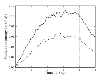
Figure 1.— Energy in the turbulent fluctuations versus time. The solid and dashed lines correspond to the total kinetic energy and magnetic energy, respectively. The vertical dotted line marks the time at which the particle integration begins. After that time the turbulence decays, to avoid spurious particle heating due to the temporal driving (see Appendix A).

Our collisionless charged particles evolve according to:

$$\frac{d\boldsymbol{u}}{dt}=\frac{q}{m}\boldsymbol{E}+\frac{q}{mc}\boldsymbol{u}\times\boldsymbol{B}$$ (9)

where $\boldsymbol{u}$ is the particle’s velocity and the remaining symbols have their standard meanings. In the particle integrator, the fields $\boldsymbol{E}$ and $\boldsymbol{B}$ are interpolated in space and time from their known values on the grid to the particle’s position. We obtain $\boldsymbol{E}$ from $\boldsymbol{v}$ and $\boldsymbol{B}$ on the grid by using:

$$\boldsymbol{E}=-\frac{1}{c}\boldsymbol{v}\times\boldsymbol{B}+\frac{\eta}{4\pi}\boldsymbol{\nabla}\times\boldsymbol{B}$$ (10)

The particle’s charge-to-mass ratio ($q/m$ in equation eq. [9]) is a free parameter. Our simulations simultaneously evolve different types of particles, with charge-to-mass ratios spanning several orders of magnitude. To make the results easier to interpret, we convert the charge-to-mass ratio to a normalized gyrofrequency: $\Omega_{0}=qB_{0}/mc$. The actual gyrofrequency $\Omega$ of a particle is close to $\Omega_{0}$, but may differ due to local turbulent fluctuations in the $\boldsymbol{B}$ field.

In our runs, particles all have positive charge. Since anisotropic Alfvénic turbulence consists of slow waves and linearly polarized Alfvén waves, the sense of the gyration (due to the sign of the charge) should make no difference to the particle heating and acceleration. To confirm this, we compared simulations with negatively charged particles to those with positively charged particles, and observed no significant differences.

3.2.1 Integration method

We first implemented the 4^th-order Runge-Kutta method and found that it was not suitable for this specific problem. We performed tests using a constant, uniform magnetic field (instead of the turbulent fields). Those tests showed a small but steady decrease in the gyroradius and the energy of the particles since the sign of the error is always in the same direction. With, e.g., 10 time steps per gyration, the energy decreased by 1 percent per gyration. This numerical bias is particularly dangerous given our goal of studying particle heating.

We thus replaced the Runge-Kutta method by the following implicit leap-frog numerical scheme, where positions are defined at integer time and velocities at half integer time:

$$\frac{\boldsymbol{u}^{n+1/2}-\boldsymbol{u}^{n-1/2}}{\Delta t} =\frac{q}{m}\boldsymbol{E}^{n}$$

$$+\frac{q}{mc}\frac{(\boldsymbol{u}^{n+1/2}+\boldsymbol{u}^{n-1/2})}{2}\times\boldsymbol{B}^{n}$$ (11)

$$\frac{\boldsymbol{x}^{n+1}-\boldsymbol{x}^{n}}{\Delta t} =\boldsymbol{u}^{n+1/2}$$ (12)

where a superscript $n$ indicates that the variable is defined at time level $n$.

The specific implementation of equation (3.2.1) that we use is the Boris particle pusher (Boris, 1970). Unlike the Runge-Kutta method, this scheme is symmetric in time and symplectic, thus conserving energy and adiabatic invariants to machine precision. Another advantage of this method is that the fields only need to be interpolated once per timestep, which makes it considerably faster than the 4^th-order Runge-Kutta method.

We choose the particle timestep $\Delta t$ so as to properly resolve the gyration. In order to also ensure that the particle timestep is smaller than the MHD timestep, we use:

$$\Delta t=\mathrm{min}\left(\frac{1}{40}\frac{2\pi}{\Omega_{0}},\frac{1}{10}\Delta t_{\mathrm{MHD}}\right)$$ (13)

which produces at least 40 steps per gyration. Tests using simplified field configurations confirmed the accuracy of this method. Some of our tests are described in §B of the Appendix.

3.2.2 Interpolation

The $\boldsymbol{B}$ and $\boldsymbol{E}$ fields are interpolated from their values on the grid and at the discrete MHD timesteps to the particle’s position. We use the Triangular Shaped Cloud (TSC) interpolation method (Hockney & Eastwood, 1981) in space and time. More details on the algorithm can be found in §C of the Appendix.

In ideal MHD, $E_{\parallel}=0$. Although this is indeed true on the grid, the interpolated $\boldsymbol{E}$ may have a non-zero component along the interpolated $\boldsymbol{B}$. Because the particles’ motion parallel to the magnetic field is unimpeded, this component, although small, can produce significant acceleration. In order to avoid non-physical parallel energization, we compute $\boldsymbol{E}\cdot\boldsymbol{B}$ on the grid (this is zero in ideal MHD, but non-zero in resistive MHD) and interpolate it to the particle’s position. We then modify the component of $\overline{\boldsymbol{E}}$ parallel to $\overline{\boldsymbol{B}}$:

$$\widetilde{\boldsymbol{E}}=\overline{\boldsymbol{E}}+\left(\overline{(\boldsymbol{E}\cdot\boldsymbol{B})}-\overline{\boldsymbol{E}}\cdot\overline{\boldsymbol{B}}\right)\frac{\overline{\boldsymbol{B}}}{||\overline{\boldsymbol{B}}||^{2}}$$ (14)

where the overline symbolizes interpolation and $\widetilde{\boldsymbol{E}}$ is the new electric field. This ensures that:

$$\widetilde{\boldsymbol{E}}\cdot\overline{\boldsymbol{B}}=\overline{(\boldsymbol{E}\cdot\boldsymbol{B})}$$ (15)

i.e., that the parallel component of $\widetilde{\boldsymbol{E}}$ is correct.

3.3. Measurement and Initialization of the Particles

We initialize the particles uniformly over the entire computational domain. We then give them a parallel velocity $u_{\parallel}$ and a gyration velocity $u_{\perp}$ drawn from the distributions discussed below.

Since the motion of a particle is in fact the superposition of a rapid gyration and a slowly varying drift, calculating the gyration velocity $u_{\perp}$ requires knowledge of the drift velocity: $u_{\perp}=||\boldsymbol{u}_{\perp,tot}-\boldsymbol{u}_{d}||$. ($\boldsymbol{u}_{\perp,tot}$ and $\boldsymbol{u}_{d}$ are the total perpendicular velocity of the particle and its drift velocity, respectively.) We take into account the dominant $\boldsymbol{E}\times\boldsymbol{B}$ drift but neglect the other drifts ($\nabla B$, curvature drift, polarization drift, …), which are small for the particles considered here. For simplicity, we also neglect the $\boldsymbol{E}\times\boldsymbol{B}$ drift due to the resistive part of $\boldsymbol{E}$, and adopt the following definition:

$$u_{\perp}=||\boldsymbol{u}_{\perp,tot}-\boldsymbol{v}_{\perp}||$$ (16)

where $\boldsymbol{v}_{\perp}$ is the perpendicular velocity of the fluid.

We use two different kinds of initial velocity distributions. For some of our calculations, our aim is to isolate the statistical effect of the turbulence on a certain type of particle. In this case, all of the particles have the same initial parallel velocity and magnetic moment:

$$f_{0}(\boldsymbol{x},\boldsymbol{u})\propto\delta\left(u_{\parallel}-u_{\parallel,0}\right)\delta\left(u_{\perp}-\sqrt{\mu_{0}B(\boldsymbol{x})}\right)$$ (17)

where $u_{\parallel,0}$ and $\mu_{0}$ specify the initial particle properties. We give the particles the same magnetic moment, not the same gyration velocity, because analytic theory predicts that $\mu$ should be conserved for particles with high $\Omega_{0}$ (§2). With this initialization we can easily check whether the interaction with the turbulence indeed conserves $\mu$. This test has been extensively performed while developing our methods.

By contrast, in other calculations, we study the integrated heating over a “realistic” distribution of particles. Here, we choose to assign the velocities according to an isotropic Maxwell-Boltzmann distribution:

$$f_{MB}(\boldsymbol{x},\boldsymbol{u})\propto\exp\left[-\frac{\left(u_{\perp}^{2}+u_{\parallel}^{2}\right)}{2c_{s}^{2}}\right]$$ (18)

In all cases the particles are split into $N$ groups, where in each group, particles all have the same physical properties such as charge-to-mass ratio (i.e., $\Omega_{0}$) or initial velocity. Each of the N groups contains particles with different values of the physical property being studied in the particular simulation (e.g., $\Omega_{0}$ or velocity).

4. Results

In the following sections we describe the interaction between the turbulence and particles with different gyrofrequencies $\Omega_{0}$ and velocities (§4.1). We also compare simulations with and without explicit resistivity (§4.2), simulations with different background magnetic field strengths (§4.3), and simulations with different grid resolution (§4.4). Finally, we study the net effect of the turbulence on a thermal distribution of particles (§4.5). To help guide the reader’s intuition, we note that our fiducial calculations (see Table 1) have $\beta\sim 1$ and turbulence with outer-scale velocities $\delta v\sim 0.5c_{s}$; the outer-scale eddy turnover time is $\sim 2L/c_{s}$. We consider particles with a range of velocities $\sim 0.1-10\,c_{s}$. High velocity particles ($\gg c_{s}$) transit the box many times in the course of the simulation; doing so, they may unphysically sample a similar realization of the turbulent fluctuations. We thus focus on lower velocity particles where the periodic box boundary conditions we employ are more reliable. This corresponds primarily to the velocities of protons or minor ions, rather than electrons, which have typical velocities $\sim 40\,c_{s}$ for $T_{e}\sim T_{p}$.

The range of gyrofrequencies we consider is $\sim 10-10^{4}\,c_{s}/L$. For a resolution of 256³, the highest linear frequency on the computational domain is $\omega_{max}\simeq k_{\parallel,max}v_{A}\sim 350\,c_{s}/L$ where we have used the critical balance conjecture (§2) to estimate that for anisotropic Alfvénic turbulence, $k_{\parallel,max}\simeq k_{max}^{2/3}\,k_{min}^{1/3}$ ($k_{max}\simeq\pi/\Delta x$ is the highest wavenumber given a resolution $\Delta x$ and $k_{min}\simeq 2\pi/(L/4)$ is the wavenumber at which the turbulence is driven). Thus the particle gyrofrequencies we consider range from particles with gyrofrequencies comparable to those of resolved turbulent fluctuations to particles with $\Omega_{o}\gg\omega_{max}$. From linear theory, the latter are expected to have primarily parallel heating because of the conservation of $\mu$ (§2).

Table 1Properties of the Fiducial Calculation

Parameter	Value
$\beta$	$1.0$
$\dot{E}$	$0.1\,\rho L^{2}c_{s}^{3}$
$\eta$	0 (ideal MHD)
Resolution	$256^{3}$ zones
Integration time	$1.0\,L/c_{s}$
Number of particles	$512\times 10^{3}$

4.1. Fiducial Results

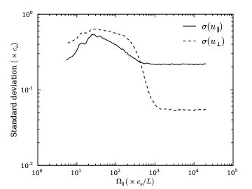
Figure 2.— Standard deviation of the parallel $u_{\parallel}$ (solid line) and perpendicular $u_{\perp}$ (dashed line) velocities at the end of the simulation, as a function of the particles’ gyrofrequency $\Omega_{0}$; the particles initially have delta functions in velocity with $u_{\parallel,0}=1.0\,c_{s}$ and $\mu_{0}=1.0\,c_{s}^{2}/B_{0}$ ($u_{\perp,0}\simeq 1.0\,c_{s}$). The strong diffusion for low $\Omega_{0}$ particles is consistent with linear theory predictions for cyclotron resonance; $\sigma(u_{\parallel})\gg\sigma(u_{\perp})$ for high $\Omega_{0}$ particles is consistent with linear theory predictions for $\mu\nabla_{\parallel}B$ acceleration at the Landau resonance (see §4.1 for details). The parameters of this calculation are summarized in Table 1.

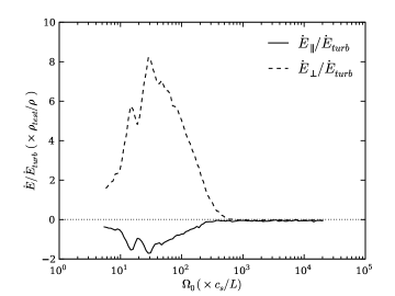
Figure 3.— Parallel (solid) and perpendicular (dashed) heating rates as a function of the particles’ gyrofrequency $\Omega_{0}$; the particles initially have delta functions in velocity with $u_{\parallel,0}=1.0\,c_{s}$ and $\mu_{0}=1.0\,c_{s}^{2}/B_{0}$ ($u_{\perp,0}\simeq 1.0\,c_{s}$). The heating rates are normalized by $\dot{E}_{turb}$, the energy dissipation rate in the turbulence. The heating rates are averaged over the full $1.0L/c_{s}$ of the calculation. The parameters of this calculation are summarized in Table 1.

The first calculations we describe are summarized in Table 1. We consider an initial delta function of particles interacting with Alfvénic turbulence having $\delta v\simeq 0.5c_{s}$ in the presence of a mean magnetic field with $\beta=1$. This interaction leads to both a stochastic diffusion in velocity space and a change in the mean energy of the particles; the magnitude of these changes depends on the cyclotron frequency $\Omega_{0}$ of the particles and their initial velocity. Figure 2 shows the standard deviation of $u_{\perp}$ and $u_{\parallel}$, for $u_{\parallel,0}=c_{s}$ and $\mu_{0}=c_{s}^{2}/B_{0}$ ($u_{\perp,0}\simeq c_{s}$), as a function of $\Omega_{0}$, at the end of the integration (after $1.0L/c_{s}$). Figure 3 shows the parallel and perpendicular heating rates for the same calculations $\left(\dot{E}_{\parallel,\perp}=\frac{d\,}{dt}\sum_{particles}\frac{1}{2}mu_{\parallel,\perp}^{2}\right)$. To make the heating rates easier to interpret, we normalize them by the average energy dissipation rate in the decaying turbulence. Because our calculations are for test particles, the heating rate can be scaled to any $\rho_{test}/\rho$, i.e., to any test particle density.

The dispersion (Fig. 2) and heating (Fig. 3) produced by the turbulence depend on the gyrofrequency of the particles. Particles with low gyrofrequency $\Omega_{0}\lesssim 300\,c_{s}/L$ are the most strongly heated, with most of the heating being in the perpendicular direction (i.e., $u_{\perp}$ increases rather than $u_{\parallel}$). The heating also depends on the gyrofrequency of the particle. By contrast, particles with high gyrofrequency $\Omega_{0}\gtrsim 300\,c_{s}/L$ have a significantly lower heating rate that is independent of $\Omega_{0}$; in addition, most of the dispersion/heating is in the direction of the magnetic field. We distinguish between the two classes of particles in Figures 2 & 3 by characterizing the low $\Omega_{0}$ particles as “cyclotron-resonant” and the high $\Omega_{0}$ particles as “Landau-resonant” (the reasons for these particular identifications will become clear shortly).

The significant heating of low $\Omega_{0}$ particles in Figures 2 & 3 is consistent with the analytic expectations for cyclotron resonance (§2). To confirm this, we note that the range of Alfvén frequencies present in the simulation is $\sim 4-350\,c_{s}/L$. This is comparable to the range of $\Omega_{0}$ in Figures 2 & 3 over which there is strong heating and diffusion. The heating is also primarily perpendicular heating, as expected analytically. The negative parallel heating for the cyclotron-resonant particles in Figure 3 is a consequence of pitch-angle scattering, as we demonstrate in more detail below.

Figures 2 & 3 show that particles with high gyrofrequency $(\Omega_{0}\gtrsim 10^{3}\,c_{s}/L)$ are significantly less affected by the turbulence than the low $\Omega_{0}$ cyclotron-resonant particles. This is particularly true for the perpendicular velocity $u_{\perp}$: $\sigma(u_{\perp})\ll\sigma(u_{\parallel})$ at high $\Omega_{0}$. We interpret this low dispersion as a nonlinear analogue of the absence of perpendicular heating in linear theory (§2), which is ultimately due to the adiabatic invariance of the magnetic moment. In fact, $\sigma(u_{\perp})$ at high $\Omega_{0}$ in Figure 2 is only modestly larger than the initial dispersion in $u_{\perp}$; because we initialize the particles with a fixed $\mu$, there is an initial dispersion in $u_{\perp}$ due to differences in $B$ in the turbulent plasma.

To assess the changes in $\mu$ explicitly, Figure 4 shows the standard deviation of $\mu$ and the change in the mean of $\mu$ for the same calculations as in Figures 2 & 3. At the end of the calculation, after 1.0 $L/c_{s}$, the mean $\mu$ of the Landau-resonant (large $\Omega_{0}$) particles has changed by $\lesssim 1\%$; the dispersion introduced by the interaction with the turbulence is somewhat larger $\sim 10\%$. These small changes are qualitatively consistent with the prediction of linear theory that high gyrofrequency particles evolve adiabatically and thus conserve their magnetic moment. Nonetheless, the small changes in $\mu$ in Figure 4 appear to be real and represent a quantitative difference relative to linear theory. We have carried out a number of tests to confirm that the changes in $\mu$ shown in Figure 4 are not numerical; e.g., the results are independent of the timestep in the particle integrator and of the Courant number in the integration of the turbulence. In addition, $\sigma(\mu)\propto\delta v$, consistent with how the parallel diffusion depends on the amplitude of the turbulence; this argues against violation of $\mu$ conservation due to finite amplitude waves, as has been proposed in other contexts (e.g., Johnson & Cheng 2001). One possible explanation for the changes in $u_{\perp}$ is that the delta function resonances in linear theory (eq. [1]) are significantly broadened in the nonlinear turbulence (as we show in more detail shortly). Recall from equation (4) that the change in $u_{\perp}$ due to interaction with a single Fourier component of the turbulence is $du_{\perp}/dt\propto[\omega-k_{\parallel}u_{\parallel}]$. In linear theory this vanishes because non-zero energy exchange with a fluctuation requires $\omega=k_{\parallel}u_{\parallel}$; this restriction is relaxed in strong Alfvénic turbulence (e.g., Chandran 2000) so that small changes in $u_{\perp}$ may be possible.

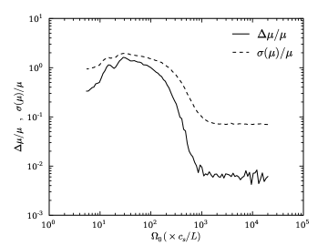
Figure 4.— Standard deviation of the magnetic moment $\mu$ at the end of the simulation (dashed line) and the change in its mean (solid line), as a function of the particles’ gyrofrequency $\Omega_{0}$; the particles initially have delta functions in velocity with $u_{\parallel,0}=1.0\,c_{s}$ and $\mu_{0}=1.0\,c_{s}^{2}/B_{0}$ ($u_{\perp,0}\simeq 1.0\,c_{s}$). The large changes in $\mu$ at low $\Omega_{0}$ are due to cyclotron resonance. Linear theory predicts that $\mu$ is conserved for high $\Omega_{0}$, which is not fully consistent with the numerical results; see §4.1 for an interpretation. The parameters of this simulation are summarized in Table 1.

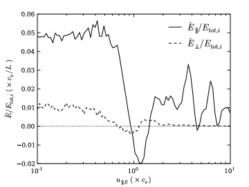
Figure 5.— Heating rates in the parallel (solid line) and perpendicular (dashed line) directions as a function of the initial parallel velocity $u_{\parallel,0}$, for Landau-resonant particles $(\Omega_{0}=4.0\times 10^{4}\,c_{s}/L)$. Although $u_{\parallel,0}$ varies, all particles initially have the same magnetic moment, $\mu_{0}=1.0\,c_{s}^{2}/B_{0}$ (and thus $u_{\perp,0}\simeq 1.0\,c_{s}$). Linear theory predicts that only particles with $u_{\parallel,0}=\omega/k_{\parallel}\simeq 0.8c_{s}$ (the Landau resonance) should exchange energy with the waves. By contrast, particles with all $u_{\parallel,0}$, and particularly those with $u_{\parallel,0}\lesssim c_{s}$, interact strongly with the turbulence. The heating rates are normalized by the total initial energy of the particle $E_{tot,i}=E_{\perp,i}+E_{\parallel,i}$, and are averaged over the whole integration. The properties of this simulation are summarized in Table 1.

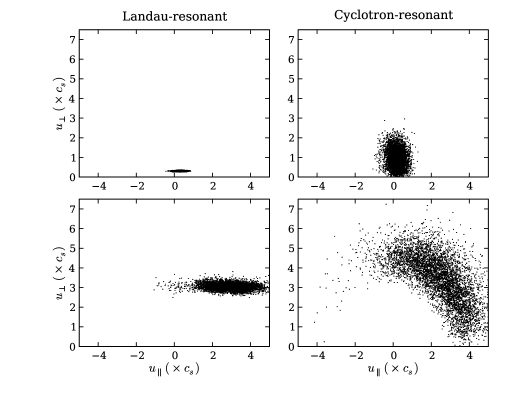
Figure 6.— Scatter plots in velocity space ($u_{\parallel}$, $u_{\perp}$) for Landau-resonant particles ($\Omega_{0}=2.0\times 10^{4}\,c_{s}/L$; left panels) and cyclotron-resonant particles ($\Omega_{0}=60\,c_{s}/L$; right panels) at the end of the simulation. The initial distribution function is a delta function. Landau-resonant particles primarily diffuse in $u_{\parallel}$ while cyclotron resonant particles undergo pitch angle scattering which tends to isotropize the distribution function. In the upper panels, the particles initially have low velocities, $u_{\perp,0}=u_{\parallel,0}=0.3\,c_{s}$. In the lower panels, the particles initially have high velocities, $u_{\perp,0}=u_{\parallel,0}=3.0\,c_{s}$. The remaining parameters are summarized in Table 1.

As described in §2, analytic theory predicts that high $\Omega_{0}$ particles interact with anisotropic Alfvénic turbulence primarily via $\mu\nabla_{\parallel}B$ acceleration by the slow magnetosonic modes. Anisotropic slow waves have the dispersion relation $\omega\simeq c_{s}v_{A}|k_{\parallel}|(c_{s}^{2}+v_{A}^{2})^{-1/2}$ (e.g., Lithwick & Goldreich 2001), which reduces to $\omega\simeq 0.8|k_{\parallel}|c_{s}$ for $\beta=1$. Thus for our fiducial calculation, the condition for high $\Omega_{0}$ Landau resonance ($n=0$ in eq. [1]) becomes:

$$u_{\parallel}\simeq\pm 0.8c_{s}.$$ (19)

Note that the resonant condition does not depend on $k$, but only on $u_{\parallel}$: the resonant particles simultaneously interact with all modes, but only a single parallel velocity is picked out in linear theory. Figure 5 shows the parallel and perpendicular heating as a function of the initial parallel velocity $u_{\parallel,0}$ for our fiducial calculation, taking a fixed $\mu_{0}=1.0\,c^{2}_{s}/B_{0}$ and a sufficiently high $\Omega_{0}=4.0\times 10^{4}\,c_{s}/L$ that there is no cyclotron resonance. Contrary to linear theory, particles with a wide range of velocities $\sim 0.1-10\,c_{s}$ receive significant energy; in particular, for $u_{\parallel,0}\lesssim 0.8c_{s}$ (the resonant velocity in linear theory), the heating is relatively independent of $u_{\parallel,0}$. The wide range of velocities at which the particles couple to the turbulence is qualitatively consistent with the idea that the linear resonances (eq. [1]) are highly broadened in Alfvénic turbulence because the nonlinear decorrelation time is comparable to or shorter than the linear period of the Alfvén and slow waves (e.g., Chandran 2000). We defer a more detailed test of resonance broadening models to future work. Although the linear resonance no longer manifests itself as a delta function, Figure 5 shows that at nearly all velocities, the heating of high $\Omega_{0}$ particles is primarily parallel to the local magnetic field, consistent with linear theory predictions.

Figure 6 shows the positions of the individual particles in velocity space at the end of the fiducial simulation, for both high $\Omega_{0}$ Landau-resonant particles (left column) and low $\Omega_{0}$ cyclotron-resonant particles (right column). The top row is for low velocity particles with $u_{\parallel,0}\simeq u_{\perp,0}\simeq 0.3\,c_{s}$ while the bottom row is for high velocity particles with $u_{\parallel,0}\simeq u_{\perp,0}\simeq 3\,c_{s}$. For Landau-resonant particles, the dispersion occurs almost exclusively in the parallel direction, as we have previously seen. For the cyclotron-resonant particles, the diffusion in velocity space depends somewhat on the velocity of the particles. For $u_{\parallel,0}\lesssim v_{A}$ (top right), the particles are preferentially dispersed in the perpendicular direction due to the cyclotron resonance. However for $u_{\parallel,0}>v_{A}$ (bottom right), the velocity diffusion is dominated by pitch angle scattering: the velocity distribution is isotropized more rapidly than the total energy changes. This difference in the results of cyclotron resonance for sub and super-Alfvénic particles is a well-known result of quasilinear theory (e.g., Miller & Roberts 1995).

4.2. Resistive Simulations

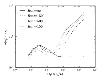
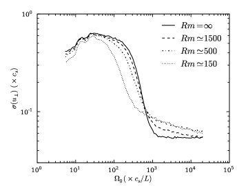
Figure 7.— Standard deviation of the parallel $u_{\parallel}$ (top panel) and perpendicular $u_{\perp}$ (bottom panel) velocities at the end of the simulation, as a function of the particles’ gyrofrequency $\Omega_{0}$. The curves are plotted for different resistivities $\eta$, which are converted to magnetic Reynolds numbers, as computed on the outer scale of the turbulence. The solid line is for $\eta=0$ (ideal MHD), while the dashed, dot-dashed and dotted lines have increasing resistivity. The presence of $\eta\neq 0$ produces an $E_{\parallel}$ that leads to significant parallel heating and diffusion at high $\Omega_{0}$, but the properties of the low $\Omega_{0}$ cyclotron-resonant particles do not depend significantly on $\eta$. The particles initially have delta functions in velocity with $u_{\parallel,0}=1.0\,c_{s}$ and $\mu_{0}=1.0\,c_{s}^{2}/B_{0}$ ($u_{\perp,0}\simeq 1.0\,c_{s}$). Aside from $\eta$, the parameters of this simulation are the same as in Table 1.

In the ideal MHD simulations described in the previous sub-section, $E_{\parallel}=0$ because of our constrained transport algorithm; this is also preserved to machine accuracy by our interpolation methods (§3). Numerical reconnection is nonetheless present on small scales. To understand the effects of reconnection and small-scale current sheets on our results in a more controlled manner, we have carried out a number of simulations with finite resistivity $\eta$. It is important to stress that the physics of reconnection is not adequately represented by a spatially and temporally constant value of $\eta$. Thus our calculations with finite $\eta$ should not be interpreted as physical. Rather, they allow us to isolate the potential importance of reconnection for some of our results and assess whether the interpretations given in the previous sub-section are correct.

We parameterize our chosen values of $\eta$ using the magnetic Reynolds number of the turbulence on the outer scale: $Rm\equiv L\delta v/[\eta c/4\pi]$. We chose values of $\eta$ so that $Rm\sim 1$ on the grid scale, i.e., so that small-scale current sheets are marginally resolved; this implies

$$\frac{\Delta x\,\delta v_{k_{max}}}{(\eta c/4\pi)}\sim 1$$ (20)

where $\Delta x$ is the size of a cell and $k_{max}\simeq\pi/\Delta x$. We estimate $\delta v_{k_{max}}$ assuming a Kolmogorov cascade $\delta v_{k}\approx\delta v(kL)^{-1/3}$. For our fiducial resolution of $256^{3}$, $Rm\sim 1$ on the grid scale thus corresponds to $Rm\sim 1500$ at the outer scale of the turbulence.

Figure 7 compares the velocity dispersion in the parallel and perpendicular directions at the end of simulations with different values of $\eta$, for particles with $u_{\parallel,0}=1.0\,c_{s}$ and $\mu_{0}=1.0\,c_{s}^{2}/B$. The most striking result is the very strong parallel dispersion for particles with high gyrofrequency. This is a consequence of the non-zero parallel electric field in resistive MHD: $E_{\parallel}=\frac{\eta}{4\pi}(\boldsymbol{\nabla}\times\boldsymbol{B})_{\parallel}$. As a result, particles are freely accelerated in the parallel direction by the $qE_{\parallel}$ force (see eq. [3]). The parallel acceleration thus depends strongly on the particle’s charge-to-mass ratio $q/m$ – or equivalently on its $\Omega_{0}$. This dependence is clearly visible in Figure 7.

The perpendicular velocity $u_{\perp}$ is much less affected by resistivity, since the additional perpendicular electric field $\boldsymbol{E}_{\perp}=\frac{\eta}{4\pi}(\boldsymbol{\nabla}\times\boldsymbol{B})_{\perp}$ averages to zero over a gyration. The strongest effect evident in Figure 7 is that, for $\Omega_{0}\sim 100\,c_{s}/L$, the perpendicular diffusion becomes weaker as the resistivity increases. The most probable explanation is that resistive dissipation preferentially damps the high $k$ modes, which are precisely the modes that resonate with particles having $\Omega_{0}\sim 100\,c_{s}/L$.

Overall, our simulations with an explicit resistivity demonstrate that, in resistive MHD, current sheets lead to parallel heating by the non-zero $E_{\parallel}$. This is in addition to the parallel heating by $\mu\nabla_{\parallel}B$ forces and the perpendicular heating and pitch-angle scattering by cyclotron-resonant waves highlighted in the previous sub-section.

4.3. Variations in $\beta$

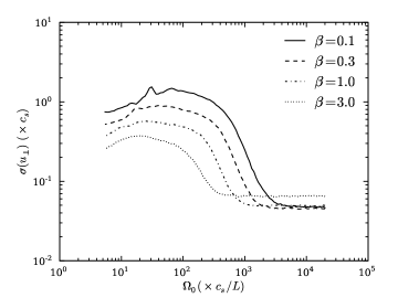
Figure 8.— Standard deviation of the perpendicular velocity $u_{\perp}$ at the end of the simulation as a function of the particles’ gyrofrequency $\Omega_{0}$, for $u_{\parallel,0}=0$ (to minimize Doppler shift) and $u_{\perp,0}\simeq 1.0\,c_{s}$. The different curves correspond to different values of $\beta$. Linear theory predicts that cyclotron resonance with Alfvén waves requires $|k_{\parallel}|v_{A}\simeq\Omega_{0}$, consistent with the increasing heating/dispersion at high $\Omega_{0}$ for decreasing $\beta$ (i.e., increasing $v_{A}$). $\dot{E}$ is adjusted so that all calculations have approximately the same Alfvénic Mach number.

We carried out a number of calculations at different $\beta$ to assess whether the particle heating physics identified in §4.1 depends significantly on $\beta$. Because we are focusing on weakly compressible Alfvénic turbulence, we kept the Alfvénic Mach number $\delta v/v_{A}$ at the saturation of the turbulence constant when varying $\beta$ (by appropriately varying $\dot{E}$). There were no significant changes in any of our results as a function of $\beta$. To illustrate one example, Figure 8 shows how the standard deviation of $u_{\perp}$ at the end of the simulation depends on the background field. In this calculation, the particles initially have $\mu_{0}=1.0\,c^{2}_{s}/B_{0}$ and $u_{\parallel,0}=0$, the latter to avoid any Doppler shifts in the cyclotron resonance.

For cyclotron resonant particles, the decreasing magnitude of $\sigma(u_{\perp})$ for higher $\beta$ in Figure 8 is due to the fact that, to keep $\delta v/v_{A}$ constant, the energy in the turbulent fluctuations is lower for high $\beta$. The cyclotron resonance clearly shifts towards higher $\Omega_{0}$ as $\beta$ decreases. This can be understand from equation (5) and the assumption of Alfvénic turbulence: resonance requires $|k_{\parallel}|v_{A}\sim\Omega_{0}$ and thus the resonant particles should have $\Omega_{0}\propto\beta^{-1/2}$. This scaling is reasonably consistent with the shift in Figure 8.

4.4. The Effects of Numerical Resolution

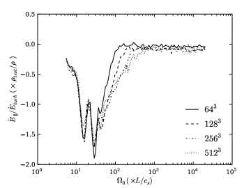
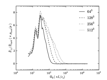
Figure 9.— Parallel (upper panel) and perpendicular (lower panel) heating rates, as a function of the particles’ gyrofrequency $\Omega_{0}$, for $u_{\parallel,0}=1.0\,c_{s}$ and $u_{\perp,0}\simeq 1.0\,c_{s}$. The different curves correspond to different resolutions. With increasing resolution, higher frequencies are present on the computational domain, which increases the range in $\Omega_{0}$ over which there is perpendicular heating due to the cyclotron resonance. By contrast, the parallel heating at high $\Omega_{0}$ is relatively independent of resolution. The heating rates are averaged over the whole integration (i.e., for $1.0\,L/c_{s}$), and are normalized by $\dot{E}_{turb}$, the energy dissipation rate in the turbulence. Apart from resolution, the properties of these calculations are summarized in Table 1.

Finite numerical resolution limits the conclusions we can draw for several reasons, even given our restriction to scales where MHD is valid. In particular, higher resolution changes the properties of the turbulence, since we can resolve higher $k$ modes. For the same reason higher resolution increases the range of linear and nonlinear frequencies found in the turbulence, and thus the range of particles that can be cyclotron resonant.

Figure 9 shows the parallel and perpendicular heating rates for different resolutions. Going to higher resolution does not significantly affect the parallel heating rate at high $\Omega_{0}$. This is reasonably consistent with linear theory: Barnes (1966) showed that the linear collisionless damping of the slow magnetosonic mode is independent of the magnitude of ${\bf k}$ (although it depends on its direction). Thus increasing the range of ${\bf k}$ contained in the domain should not significantly change the heating rate, since all scales contribute significantly. By contrast, Figure 9 shows that the range of gyrofrequencies $\Omega_{0}$ that can be cyclotron resonant increases with resolution: higher frequency particles are cyclotron-resonant at higher resolution because the range of resolved ${\bf k}$, and thus the range of resolved frequencies, increases at higher resolution.

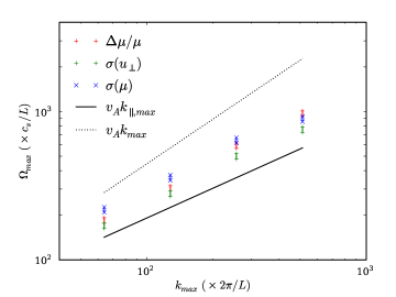
Figure 10.— Maximum gyrofrequency $\Omega_{max}$ for cyclotron-resonant particles as a function of resolution (colored symbols); the resolution is quantified by the maximum wavenumber resolved in the simulation $k_{max}\equiv\pi/\Delta x$. Also shown is the maximum frequency of Alfvén waves as a function of resolution in an isotropic cascade (dotted line) and for anisotropic Alfvénic turbulence (solid line; $k_{\parallel max}\simeq k_{max}^{2/3}k_{min}^{1/3}$). The numerical results favor the anisotropic turbulence models. $\Omega_{max}$ is the value of the particle gyrofrequency $\Omega_{0}$ at which $\Delta\mu/\mu$, $\sigma(u_{\perp})$, or $\sigma(\mu)$ is larger than its $\Omega_{0}\rightarrow\infty$ value by a factor $\sim 2$ (see §4.4 for details).

Quantifying the range of $\Omega_{0}$ that are cyclotron-resonant at a given resolution is critical for understanding the implications of our results for solar and astrophysical problems (§5.2). Towards this end we define a maximum cyclotron frequency $\Omega_{max}$: this is the value of $\Omega_{0}$ at which $\Delta\mu/\mu$, $\sigma(u_{\perp})$, or $\sigma(\mu)$ is larger than its $\Omega_{0}\rightarrow\infty$ value by a factor of $2$. The exact definition of $\Omega_{max}$ is somewhat arbitrary, but our definition captures the key result seen in many of the plots in this paper (e.g., Fig. 2 & 4): the dispersion/heating in $\mu$ and $u_{\perp}$ are small at high $\Omega_{0}$ (for Landau-resonant particles) and then increase rapidly for smaller $\Omega_{0}$ as $\Omega_{0}$ becomes comparable to the frequency of Alfvén waves on the computational domain. By considering three different physical quantities ($\Delta\mu/\mu$, $\sigma(u_{\perp})$, and $\sigma(\mu)$) in defining $\Omega_{max}$ we hope to bracket some of the uncertainty in our estimate of $\Omega_{max}$.

Figure 10 shows these three different definitions of $\Omega_{max}$ as a function of $k_{max}\equiv\pi/\Delta x$, for our fiducial calculation with $\beta=1$, $u_{\parallel,0}=1.0\,c_{s}$, and $u_{\perp,0}\simeq 1.0\,c_{s}$. There is a clear tend of increasing $\Omega_{max}$ with $k_{max}$. Also shown in Figure 10 are two theoretical predictions for the maximum Alfvén wave frequency as a function of resolution. The first (dotted line) assumes an isotropic cascade in which case the maximum Alfvén frequency is $\simeq k_{max}\,v_{A}$. The second estimate (solid line) takes into account the anisotropy of Alfvénic turbulence; critical balance implies that the maximum Alfvén frequency is $k_{\parallel,max}v_{A}\simeq k_{max}^{2/3}\,k_{min}^{1/3}\,v_{A}$, where in Figure 10 we take $k_{min}=2\pi/(L/4)$ since we drive modes with wavelengths between $L/4$ and $L$ (see §3.1).

The estimates of $\Omega_{max}$ in Figure 10 are reasonably consistent with $\Omega_{max}\simeq 2\,k_{\parallel,max}v_{A}$, which is comparable to the maximum Alfvén wave frequency in anisotropic Alfvénic turbulence. Because the discrete resonances of linear theory are “broadened” in strong MHD turbulence (Fig. 5), the maximum gyrofrequency of particles that feel the cyclotron resonance should be somewhat larger than maximum Alfvén wave frequency. This is true for the anisotropic estimate of $\Omega_{max}$ in Figure 10, but not the isotropic estimate. The non-trivial point demonstrated by Figure 10 is that (as predicted by linear theory) it is the smallest parallel length-scale in the turbulent fluctuations that determines the efficacy of cyclotron resonance, and thus perpendicular heating. This fact will be very important when we apply our results to space physics and astrophysics problems in §5.2.

4.5. Heating of a Thermal Distribution

In the previous sections we have focused on the diffusion and heating of particles that all start with approximately the same velocity, in order to isolate the physics of test particles interacting with strong Alfvénic turbulence. In order to obtain a more realistic estimate of the total heating rate in a turbulent plasma, we now consider an isotropic thermal distribution of particles ($f_{MB}$ in eq. [18]). These calculations have $\beta=1$ and the test particles have a thermal speed equal to that of the fluid; thus the thermal test particles represent protons or other particles with a similar thermal speed.

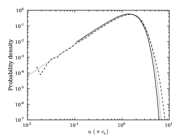
Figure 11.— Distribution functions vs. total velocity $u=\sqrt{u_{\perp}^{2}+u_{\parallel}^{2}}$, for cyclotron-resonant particles with $\Omega_{0}=250\,c_{s}/L$. The distribution function is initially thermal with the same sound speed as the fluid (solid line); the test particles thus represent protons. The dashed line is the distribution function at the end of the integration (after $1.0L/c_{s}$), while the dotted line is a thermal distribution with the same average energy as the final distribution. The cyclotron resonance leads to modest acceleration of high energy particles. The properties of the simulation are the same as in Table 1, except for the resolution, which is $512^{3}$.

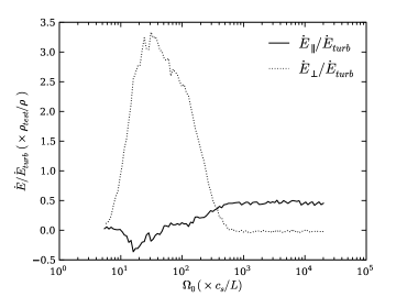
Figure 12.— Parallel (solid line) and perpendicular (dashed line) heating rates, as a function of the particles’ gyrofrequency $\Omega_{0}$. The heating rates are averaged over the last half of the simulation (i.e., for $0.5\,L/c_{s}$), and are normalized by $\dot{E}_{turb}$, the energy dissipation rate in the turbulence. The distribution function is initially thermal with the same sound speed as the fluid; the test particles thus represent protons. The Landau-resonant particles with high $\Omega_{0}$ receive primarily parallel heating while the cyclotron-resonant particles with lower $\Omega_{0}$ are largely heated in the direction perpendicular to the local magnetic field.

Figure 11 shows the evolution of the velocity distribution as the simulation proceeds, for cyclotron-resonant particles $(\Omega_{0}=250\,c_{s}/L)$. The distribution function develops a modest non-thermal tail, although most of the energy remains in the thermal population of particles. Figure 12 shows the particles’ parallel and perpendicular heating rates, divided by the average energy dissipation rate in the turbulence, as a function of the particles’ gyrofrequency $\Omega_{0}$. As before, these results can be rescaled by $\rho_{test}/\rho$ to apply them to any specific population of test particles. For high gyrofrequency $(\gtrsim 500\,c_{s}/L)$, Figure 12 shows that the heating is primarily parallel to the magnetic field; the total perpendicular heating rate fluctuates around $\simeq-0.025\,\dot{E}_{turb}\simeq-\dot{E}_{\parallel}/20$, sufficiently small that it is hard to read off of the Figure. As we have argued before, this parallel heating is due to the stochastic $\mu\nabla B$ forces created by slow magnetosonic waves. Note that the magnitude of the parallel heating rate is $\simeq 0.5\,\dot{E}_{turb}$. This is sufficiently strong that, for the parameters chosen here ($\beta=1$), a significant fraction of the energy in the slow wave cascade would be dissipated on large scales, rather than cascading to small scales.

For lower $\Omega_{0}$ ($10-300\,c_{s}/L$), Figure 12 shows that the net heating of the thermal distribution function is primarily perpendicular to the magnetic field. The heating is very strong, $\simeq 3\dot{E}_{turb}$ (for $\rho_{test}\simeq\rho$) and $\simeq 6$ times the heating rate in the high $\Omega_{0}$ limit. This strong perpendicular heating is, we have argued, due to cyclotron resonance. For $\rho_{test}\simeq\rho$, the energy gained by the particles significantly exceeds the energy available in the turbulence. This clearly demonstrates that the damping is sufficiently strong that the test particle approximation breaks down, if in fact the turbulent fluctuations reach $\omega\sim\Omega_{0}$. We return to this issue in §5.

5. Summary and Implications

We have carried out a detailed study of the heating of test particles by weakly compressible MHD turbulence. Our calculations integrate the equations of motion for up to $\sim 10^{6}$ particles in “real time” as the turbulence itself evolves. The heating and acceleration of particles by MHD turbulence plays a central role in theoretical models of many heliospheric and astrophysical phenomena, including solar flares (Miller & Roberts, 1995), cosmic-ray scattering and confinement in the Galaxy (Chandran, 2000), the heating and acceleration of the solar wind (Cranmer & van Ballegooijen, 2005), and the radiation produced by some accretion disks onto compact objects (Quataert & Gruzinov, 1999). Because of the many potential applications of this work, we have focused on the basic physics of particles interacting with MHD turbulence, rather than on any of these specific applications. In this section we first summarize our primary results and then briefly discuss their implications for astrophysical systems, in particular the solar wind.

Our turbulence is driven subsonically, sub-Alfvénically and with a divergence free velocity field (§3.1). Such weakly compressible MHD turbulence consists of nonlinearly interacting Alfvén and slow magnetosonic waves, with most of the energy cascading to small scales perpendicular to the local magnetic field (e.g., Goldreich & Sridhar 1995). There is an extensive body of work studying the heating of test particles using (quasi)linear theory, which predicts that energy exchange happens at discrete resonances (e.g., Stix 1992 and references therein); we review these predictions in §2. Our calculations relax many of the simplifying assumptions made in linear theory. Specifically, rather than studying the interaction between particles and a superposition of long-lived linear waves, our particles interact with strong MHD turbulence, i.e., with turbulence in which the timescale for nonlinear interactions to transfer energy to smaller scales is comparable to, or shorter than, the linear period of the waves. We have also carried out both ideal and resistive-MHD simulations in order to isolate the importance of dissipation in current sheets, rather than wave-particle resonances, for particle heating.

5.1. Summary

One of the striking conclusions of our work is that many – although not all – of the results we find for test particle diffusion and heating in fully developed MHD turbulence are qualitatively consistent with the predictions of quasilinear theory (we defer a more quantitative comparison between our numerical results and quasilinear theory to future work). More specifically, our primary results can be summarized as follows:

$\bullet$ How particles are heated depends sensitively on whether the gyrofrequency of the particle $\Omega_{0}$ is comparable to the frequency of a turbulent fluctuation $\omega$ that is resolved on the computational domain.

$\bullet$ Particles with $\Omega_{0}\sim\omega$ undergo strong perpendicular heating and pitch angle scattering, qualitatively consistent with linear theory predictions for cyclotron resonance with the linearly polarized Alfvén waves present in MHD turbulence (e.g., Fig. 2, 3, 6, & 12). In §5.2 we discuss the implications of this perpendicular heating for measurements of proton and ion temperature anisotropies in the solar corona and solar wind.

$\bullet$ Particles with $\Omega_{0}\gg\omega$ undergo strong parallel heating, qualitatively consistent with linear theory predictions for the heating produced by the $\mu\nabla_{\parallel}B$ forces (“transit time damping”) associated with the slow magnetosonic waves in MHD turbulence (e.g., Fig. 2, 3, 6, & 12).

$\bullet$ In contrast to the predictions of linear theory, we find that discrete resonances do not dominate the energy transfer between particles and waves. Instead, energy transfer occurs for a wide range of particles, even those that would be quite “off-resonance” according to linear theory (Fig. 5). This is broadly consistent with models in which the rapid decorrelation of waves in anisotropic MHD turbulence leads to significant “resonance broadening” (e.g., Chandran 2000).

$\bullet$ Linear theory predicts that particles with $\Omega_{0}\gg\omega$ undergo purely parallel heating because of the adiabatic invariance of the magnetic moment $\mu\propto u_{\perp}^{2}/B$ in the presence of low-frequency electromagnetic fluctuations. Although we do find that most of the heating is parallel to the local field for particles with $\Omega_{0}\gg\omega$ (Fig. 3 & 12) we also see small, but non-zero, changes in $u_{\perp}$ and $\mu$ even for high cyclotron-frequency particles (Fig. 4). The physical origin of this perpendicular heating is not fully clear, but we speculate that it may be a consequence of resonance broadening (§4.1). We find that the perpendicular heating and diffusion rates are $\sim 10\%$ of the parallel heating and diffusion rates for $\Omega_{0}\gg\omega$ (e.g., Fig. 5 & 12). Although this is unlikely to change any of the general conclusions about perpendicular versus parallel heating derived from linear theory, it is an interesting modification to the physical picture of how particles interact with anisotropic Alfvénic turbulence.

$\bullet$ All of the results summarized above are present in both ideal MHD simulations and in simulations that include an explicit resistivity to dissipate small-scale fluctuations in the turbulence. A finite resistivity also generates a non-zero $E_{\parallel}$ that produces strong parallel heating and diffusion of particles (Fig. 7). It is important to stress that the physics of reconnection is not adequately represented by the spatially and temporally constant resistivity present in our calculations. Indeed, particle-in-cell and Hall MHD simulations of reconnection show that particle heating in current sheets is far more subtle than can be captured by resistive-MHD simulations (Drake et al., 2009b, a). Further work is thus required to understand the particle heating and acceleration produced by current sheets that self-consistently develop on small scales in a turbulent plasma.

$\bullet$ For the particular case in which we initialize a thermal distribution of test particles having the same sound speed as the fluid in our turbulence calculations, the test particles approximate the interaction between protons and the turbulent fluctuations. For $\beta\sim 1$, Figure 12 shows that the heating rate of the test particles is $\sim 3\dot{E}_{turb}$ for cyclotron-resonant particles with low $\Omega_{0}$ and $\sim 0.5\dot{E}_{turb}$ for Landau-resonant particles with high $\Omega_{0}$ (where $\dot{E}_{turb}$ is the energy dissipation rate in the turbulence). This highlights that in a low-collisionality plasma, the wave-particle interactions are strong enough to damp a large fraction of the turbulent energy; the test particle approximation is thus a poor one.

In all of our calculations, the test particles have velocities within a factor of $\sim 10$ of the sound speed of the fluid $c_{s}$. This corresponds primarily to the velocities of protons or minor ions, rather than electrons, which have typical velocities $\sim 40\,c_{s}$ for $T_{e}\sim T_{p}$. High velocity particles ($\gg c_{s}$) transit the computational domain many times in the course of the simulation; doing so, they may repeatedly sample very similar realizations of the turbulent fluctuations. We believe that tests with larger computational domains are required in order to reliably study the turbulent diffusion and heating of high velocity particles. This limitation has two significant implications. First, our calculations do not at this point predict the relative turbulent heating of electrons and protons, which would be of considerable interest for both solar and astrophysical problems (e.g., Quataert & Gruzinov 1999; Cranmer et al. 2009). Second, our calculations are limited in their ability to predict the acceleration of particles to energies well above the thermal energy of the plasma. It is nonetheless important to highlight that when we initialize a thermal distribution of test protons that are cyclotron resonant with the turbulent fluctuations, the distribution function naturally evolves a non-thermal tail (Fig. 11).

Previous work on test particle heating in MHD turbulence simulations (Dmitruk et al., 2004) concluded that current sheets produce significant parallel heating of electrons and that ions are preferentially heated in the perpendicular direction. Our results are broadly consistent with these conclusions given Dmitruck et al’s assumed particle gyrofrequencies. Dmitruk et al. (2004) give an involved physical interpretation of the perpendicular heating in their calculations; we suspect that it is simply due to cyclotron resonance, as we have found in our calculations. Perhaps most importantly, the perpendicular ion heating found both here and in Dmitruk et al. (2004) is not, we believe, applicable to the solar wind, contrary to the claims made by Dmitruck et al. In particular, as we now explain, Dmitruk et al. (2004) did not consider the limitations imposed by finite numerical resolution when claiming that their results could be directly applied to the solar wind.

5.2. Implications

Broadly speaking, our results suggest that many of the conclusions drawn from quasilinear theory about the heating and acceleration of particles by anisotropic Alfvénic turbulence are likely to be qualitatively correct. However, many of the quantitative results may change given, e.g., the lack of the discrete resonances that strongly shape the predictions of quasilinear theory (Fig. 5). Assessing in detail the implications of our results for heating by MHD turbulence in solar and astrophysical environments will require additional work. Here we take the near-Earth solar wind as an example to illustrate the implications of our results and the limitations due to finite numerical resolution.

A number of observations indicate that the solar wind undergoes spatially extended heating. For example, in situ measurements from satellites such as Helios & Ulysses show that electrons and protons have non-adiabatic temperature profiles (e.g., Cranmer et al. 2009). Heating by anisotropic Alfvénic turbulence is one of the leading models for the origin of this non-adiabiticity (e.g., Matthaeus et al. 1999; Cranmer & van Ballegooijen 2003). In situ measurements of the solar wind at 1 AU show that the proton distribution function is on average anisotropic with respect to the local magnetic field: $T_{\perp}\simeq 0.9\,T_{\parallel}$ (Bale et al., 2009), although the sign of the anisotropy depends on the wind speed, with $T_{\perp}\gtrsim T_{\parallel}$ for $v_{wind}\gtrsim 600$ km s^-1 and $T_{\perp}\lesssim T_{\parallel}$ for $v_{wind}\lesssim 600$ km s^-1 (Kasper et al., 2002; Hellinger et al., 2006). It is not yet clear how to understand these measured temperature anisotropies in the context of heating by anisotropic Alfvénic turbulence.

Typical physical parameters for the slow solar wind at $\sim 1$ AU near Earth are $B\simeq 10^{-4}$ G, $n_{0}\simeq 20$ cm^-3, $T_{p}\simeq T_{e}\simeq 1.5\times 10^{5}$ K, $v_{A}\simeq 50$ km s^-1, $c_{s}\simeq 35$ km s^-1, $v_{\rm wind}\simeq 460$ km s^-1, and $\beta\simeq 0.4$ (e.g., Celnikier et al. 1987); the proton Larmor radius and gyrofrequency are thus $r_{L,p}\simeq 3\times 10^{6}$ cm and $\Omega_{p}\simeq 0.15$ Hz, respectively, while the electron Larmor radius and gyrofrequency are $r_{L,e}\simeq 10^{5}$ cm and $\Omega_{e}\simeq 300$ Hz, respectively. Howes et al. (2008a) reviewed a variety of observational diagnostics of the outer scale of the turbulence in the solar wind and estimated that $k_{min}^{-1}\sim 10^{10-11}$ cm. The cyclotron frequency in our calculations is expressed in units of $c_{s}/L$ where the size of our box $L\sim 2\pi/k_{min}$ is also of order the outer-scale of the turbulence $k_{min}^{-1}$. Expressed in these units, the proton and electron cyclotron frequencies in the solar wind are $\simeq 10^{4-5}\,c_{s}/L$ and $\simeq 10^{7-8}\,c_{s}/L$, respectively. The minimum value of the proton cyclotron frequency in the solar wind is thus comparable to the maximum value of the cyclotron frequency of particles that we have simulated (e.g., Fig 12). The fundamental reason for this is that, in nearly all heliospheric and astrophysical plasmas, the ratio of the proton cyclotron frequency to the outer-scale frequency of MHD turbulence is much larger than the dynamic range that can be simulated with current computational resources.

A naive application of our results to the near-Earth solar wind, using the parameters above, suggests that all particle heating by MHD turbulence corresponds to Landau-resonant particles (high $\Omega_{0}$) in the terminology of this paper. This is indeed correct, for the outer-scale turbulent fluctuations that we can simulate. If a slow wave cascade is present at $\sim 1$ AU, our $\beta=1$ simulations in Figure 12 demonstrate that most of the slow-wave energy on large-scales is likely lost to particle heating, in particular parallel heating of the protons. In addition to being important for the thermodynamics of the solar wind, the slow waves are one of the primary sources of density fluctuations in anisotropic Alfvénic turbulence (Lithwick & Goldreich, 2001); if they are indeed largely damped at large scales when $\beta\sim 1$, this suppresses the contribution of slow waves to the small-scale density fluctuations that are directly measured in the solar wind (see Chandran et al. 2009).

Although the slow wave component of the cascade can lose a significant fraction of its energy on large scales to $\mu\nabla_{\parallel}B$ acceleration of particles (Fig. 12), the Alfvén-wave component of the cascade does not produce significant particle heating until (1) the Alfvén wave frequency becomes comparable to the cyclotron frequency of particles that have a significant density (e.g., protons or helium) or (2) the perpendicular wavelength of the Alfvén waves becomes comparable to the proton Larmor radius $r_{L,p}$, at which point the Alfvén wave cascade transitions to a kinetic Alfvén wave cascade (Howes et al., 2008a).

From Figure 10 we conclude that the maximum gyrofrequency of particles that can be cyclotron-resonant with the turbulence is $\Omega_{max}\simeq 2\,k_{\perp,max}^{2/3}k_{min}^{1/3}v_{A}$, where we have identified $k_{max}\simeq k_{\perp,max}$ given the anisotropy of the Alfvénic cascade. Using the parameters for the solar wind above, we estimate that the maximum gyrofrequency of a particle that can be cyclotron-resonant when the cascade reaches $k_{\perp,max}\sim r_{L,p}^{-1}$ is $\Omega_{max}\simeq 0.02$ Hz $\ll\Omega_{p}\simeq 0.15$ Hz. As a result direct cyclotron resonance is not important at $k_{\perp,max}\sim r_{L,p}^{-1}$; instead, the dissipation of the Alfvénic component of weakly compressible MHD turbulence occurs via the kinetic Alfvén wave cascade launched when $k_{\perp,max}\sim r_{L,p}^{-1}$. Our results based on the direct integration of particle orbits in fully developed MHD turbulence support previous work that reached the same conclusion using linear theory cascade models (e.g., Quataert & Gruzinov 1999; Cranmer & van Ballegooijen 2003; Howes et al. 2008a).

The dissipation of anisotropic kinetic Alfvén wave turbulence having $k_{\perp}\gtrsim r_{L,p}^{-1}$ is still not fully understood; possibilities include Landau resonance (Howes et al., 2008a), secondary instabilities that generate cyclotron frequency waves (Markovskii et al., 2006), dissipation in current sheets (Drake et al., 2009a), and stochastic ion orbits created by sufficiently large amplitude waves (Johnson & Cheng, 2001; Voitenko & Goossens, 2004). Our results, together with the empirical evidence for energetically important kinetic Alfvén waves in the near-Earth solar wind (e.g., Sahraoui et al. 2009), strongly suggest that the anisotropic proton and ion temperatures in the solar wind are in part a consequence of heating by this kinetic Alfvén wave cascade.

Appendix A Interaction of particles with the turbulent driving

As mentioned in §3.2.1, driving the turbulence can have undesirable effects on the particles’ motion. Our default method for driving the turbulence introduces random kicks to the velocity field at each MHD timestep. This artificially introduces variations that are much faster than the MHD evolution, and potentially faster than the particles’ gyration. As a result, the conservation of the magnetic moment can be artificially modified. Figure 13 compares the standard deviation of the magnetic moment in two simulations: we either continue driving the turbulence after the particle integration is turned on (dashed) or let the turbulence decay (solid). The particles initially have $u_{\parallel,0}=1.0\,c_{s}$ and $\mu_{0}=1.0\,c_{s}^{2}/B_{0}$, with no variance in $\mu$. After an integration time $\simeq L/c_{s}$, the two simulations produce quite different dispersions in $\mu$, in particular at high $\Omega_{0}$, where the gyrofrequency is much larger than the true frequencies of the fluctuations resolved in the simulation. The continued driving introduces spurious high frequencies into the problem, which significantly change the resulting particle heating. This can be remedied by driving with a decorrelation time comparable to the outer-scale turnover time of the turbulence, but we choose to be conservative and study the particle heating in decaying turbulence.

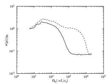
Figure 13.— Standard deviation of the magnetic moment $\mu$ as a function of the particles’ gyrofrequency $\Omega_{0}$, after an integration time of $\simeq L/c_{s}$. After the particle integration begins we either let the turbulence decay (solid line) or keep driving it (dashed line). The parameters of the simulation are summarized in Table 1. The continued driving of the turbulence (dashed line) introduces spurious high frequencies into the problem which artificially increase the magnetic moment at high $\Omega_{0}$.

Appendix B Tests

After writing the particle integrator, we verified it with a series of tests. We ran it with several simple field configurations and checked that we recovered known solutions. We also studied how the results depended on the chosen time step. Here we summarize some of our tests and their results.

B.1. Constant magnetic field

The simplest test is to confirm that one obtains the well-known helical motion in the case of a constant and uniform magnetic field and no electric field. For this problem, our method conserves the particles’ energy and magnetic moment to machine accuracy. The Boris algorithm tends to produce a slightly low gyrofrequency and a slightly large gyroradius. However, with our choice of 40 time steps per gyration, the relative error is $\simeq 10^{-3}$. Note also that this simply produces a systematic change in the definition of the charge to mass ratio of the particles; there is no secular change in time.

B.2. Alfvén wave

We let the particles evolve in the presence of a single Alfvén wave propagating parallel to the background magnetic field. The particles’ velocities are initialized according to the delta function $f_{0}$ from equation (17), so they all start with the same magnetic moment. Figure 14 shows $\sigma(\mu)$ after an integration time of $\sim L/c_{s}$ for different values of $\beta$ (and thus different values of $v_{A}$). The magnetic moment is conserved to high accuracy for particles with gyrofrequencies much larger than the frequency of the wave. We also observe several resonances that produce large changes in $\mu$. These are consistent with cyclotron resonances, and their positions scale as $\beta^{-1/2}$, as predicted by linear theory.

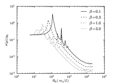
Figure 14.— Standard deviation of the magnetic moment $\mu$ as a function of the particles’ gyrofrequency $\Omega_{0}$, due to interaction with a single parallel-propagating Alfvén wave, after an integration time of $\simeq L/c_{s}$. The particles’ initial velocities are $u_{\parallel,0}=0$ and $u_{\perp,0}=1.0\,c_{s}$. The curves correspond to different values of $\beta$, but in all cases the wave has the same amplitude ($\delta v=0.1\,c_{s}$) and the same wavenumber ($k=4\times 2\pi/L$).

An important feature of Alfvén waves is that the perturbed electric field vanishes in the frame of the wave. As a consequence, the energy of a particle cannot change in this frame. Back in the frame of the fluid:

$$u_{\perp}^{2}+(u_{\parallel}-v_{A})^{2}=\epsilon$$ (B1)

where $\epsilon$ is the initial energy of the particle. Particles thus evolve on a sphere in velocity space. Figure 15 shows how cyclotron-resonant particles are scattered by an Alfvén wave in velocity space. The wave has an amplitude $\delta v=0.1\,c_{s}$ and wavenumber $k=4\times 2\pi/L$; $\beta=0.3$. The fact that particles remain on a circle centered on $v_{A}$ confirms that our integrator accurately reproduces the properties of the resonance.

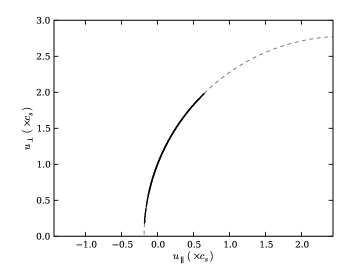
Figure 15.— Scatter plot in velocity space ($u_{\parallel}$,$u_{\perp}$), for cyclotron-resonant particles ($\Omega_{0}=60\,c_{s}/L$) interacting with a plane Alfvén wave ($\delta v=0.1\,c_{s}$; $k=4\times 2\pi/L$) at $\beta=0.3$. The gray dashed circle has its center at $(v_{A},0)$ – with $v_{A}=2.6\,c_{s}$ – and represents constant energy in the frame of the wave. The particles initially all have the same values of $u_{\parallel}$ and $\mu$; the black dots show the location of the particles after interacting with the wave for a time $\simeq L/c_{s}$. As required analytically, the particles move only along the gray dashed curve.

B.3. Particle’s timestep

As explained in §3.2.1, for particles with normalized gyrofrequency $\Omega_{0}$, our integration time step is chosen to be

$$\Delta t_{particle}=\mathrm{min}\left(\frac{1}{N_{1}}\frac{2\pi}{\Omega_{0}}\,,\,\frac{1}{N_{2}}\Delta t_{MHD}\right)$$ (B2)

where $N_{1}$ corresponds to the minimal number of particle time steps per gyration, and $N_{2}$ corresponds to the minimal number of particle time steps within one MHD time step. In our simulations, we use $N_{1}=40$ and $N_{2}=10$. For $N_{2}\gtrsim 3$, there was no significant change in the results. Similarly, so long as $N_{1}\gtrsim 10$, we found that the results were converged to better than $\sim 1\%$.

Appendix C Interpolation Method

This section gives more details on how we interpolate the fields $\boldsymbol{E}$ and $\boldsymbol{B}$ from the MHD grid to the particle’s position. We use a directionally split interpolation algorithm. The fields are averaged with weights that are the product of four 1-dimensional weights. If $(x,y,z,t)$ is the current position of the particle, $i_{0}$, $j_{0}$, $k_{0}$ the indices of the nearest cell, and $l_{0}$ the index of the nearest MHD timestep:

$$\overline{\boldsymbol{F}}=\sum_{i=i_{0}-1}^{i_{0}+1}\sum_{j=j_{0}-1}^{j_{0}+1}\sum_{k=k_{0}-1}^{k_{0}+1}\sum_{l=l_{0}-1}^{l_{0}+1}w_{i}(x)\>w_{j}(y)\>w_{k}(z)\>w_{l}(t)\,\boldsymbol{F}_{i,j,k,l}$$ (C1)

where the $\boldsymbol{F}$ stands for $\boldsymbol{E}$ or $\boldsymbol{B}$, and the overline represents interpolation.

Choosing appropriate 1-D weights is crucial. In particular, ill-chosen expressions may lead to discontinuities in the interpolated fields as particles cross from one cell to another, and have proved to produce spurious variation in the particles’ energy. As explained in §3.2.2, we use the Triangular Shaped Cloud (TSC) method, which ensures that the interpolated fields have $\mathcal{C}^{1}$ smoothness in both space and time. In the $x$ direction, for instance:

$$w_{i_{0}-1}(x) =\frac{1}{2}\left(\frac{1}{2}-\frac{(x-x_{i_{0}})}{\Delta x}\right)^{2}$$ (C2)

$$w_{i_{0}}(x) =\frac{3}{4}-\left(\frac{x-x_{i_{0}}}{\Delta x}\right)^{2}$$ (C3)

$$w_{i_{0}+1}(x) =\frac{1}{2}\left(\frac{1}{2}+\frac{(x-x_{i_{0}})}{\Delta x}\right)^{2}$$ (C4)

where $x_{i_{0}}$ is the $x$ position of the nearest cell’s center and $\Delta x$ is the grid spacing. Weights in the $y$, $z$ and $t$ directions have similar expressions.

References

- Achterberg (1981) Achterberg, A. 1981, A&A, 97, 259
- Balbus & Hawley (1998) Balbus, S. A., & Hawley, J. F. 1998, Reviews of Modern Physics, 70, 1
- Bale et al. (2009) Bale, S. D., Kasper, J. C., Howes, G. G., Quataert, E., Salem, C., & Sundkvist, D. 2009, ArXiv e-prints
- Bale et al. (2005) Bale, S. D., Kellogg, P. J., Mozer, F. S., Horbury, T. S., & Reme, H. 2005, Physical Review Letters, 94, 215002
- Barnes (1966) Barnes, A. 1966, Physics of Fluids, 9, 1483
- Blackman (1999) Blackman, E. G. 1999, MNRAS, 302, 723
- Boris (1970) Boris, J. 1970, in Proceedings of the Fourth Conference on Numerical Simulation of Plasmas (Naval Research Lab), 3–67
- Celnikier et al. (1987) Celnikier, L. M., Muschietti, L., & Goldman, M. V. 1987, A&A, 181, 138
- Chandran (2000) Chandran, B. D. G. 2000, Physical Review Letters, 85, 4656
- Chandran et al. (2009) Chandran, B. D. G., Quataert, E., Howes, G. G., Xia, Q., & Pongkitiwanichakul, P. 2009, ArXiv e-prints
- Cho & Lazarian (2003) Cho, J., & Lazarian, A. 2003, MNRAS, 345, 325
- Cho & Vishniac (2000) Cho, J., & Vishniac, E. T. 2000, ApJ, 539, 273
- Cranmer et al. (2009) Cranmer, S. R., Matthaeus, W. H., Breech, B. A., & Kasper, J. C. 2009, ArXiv e-prints
- Cranmer & van Ballegooijen (2003) Cranmer, S. R., & van Ballegooijen, A. A. 2003, ApJ, 594, 573
- Cranmer & van Ballegooijen (2005) —. 2005, ApJS, 156, 265
- Dmitruk et al. (2004) Dmitruk, P., Matthaeus, W. H., , & Seenu, N. 2004, The Astrophysical Journal, 617, 667
- Drake et al. (2009a) Drake, J. F., Cassak, P. A., Shay, M. A., Swisdak, M., & Quataert, E. 2009a, ApJ, 700, L16
- Drake et al. (2009b) Drake, J. F., Swisdak, M., Phan, T. D., Cassak, P. A., Shay, M. A., Lepri, S. T., Lin, R. P., Quataert, E., & Zurbuchen, T. H. 2009b, Journal of Geophysical Research (Space Physics), 114, 5111
- Gardiner & Stone (2005) Gardiner, T. A., & Stone, J. M. 2005, Journal of Computational Physics, 205, 509
- Goldreich & Sridhar (1995) Goldreich, P., & Sridhar, S. 1995, ApJ, 438, 763
- Hellinger et al. (2006) Hellinger, P., Trávníček, P., Kasper, J. C., & Lazarus, A. J. 2006, Geophys. Res. Lett., 33, 9101
- Higdon (1984) Higdon, J. C. 1984, ApJ, 285, 109
- Hockney & Eastwood (1981) Hockney, R. W., & Eastwood, J. W. 1981, Computer Simulation Using Particles
- Howes et al. (2008a) Howes, G. G., Cowley, S. C., Dorland, W., Hammett, G. W., Quataert, E., & Schekochihin, A. A. 2008a, Journal of Geophysical Research (Space Physics), 113, 5103
- Howes et al. (2008b) Howes, G. G., Dorland, W., Cowley, S. C., Hammett, G. W., Quataert, E., Schekochihin, A. A., & Tatsuno, T. 2008b, Physical Review Letters, 100, 065004
- Johnson & Cheng (2001) Johnson, J. R., & Cheng, C. Z. 2001, Geophys. Res. Lett., 28, 4421
- Kasper et al. (2002) Kasper, J. C., Lazarus, A. J., & Gary, S. P. 2002, Geophys. Res. Lett., 29, 170000
- Leamon et al. (1999) Leamon, R. J., Smith, C. W., Ness, N. F., & Wong, H. K. 1999, J. Geophys. Res., 104, 22331
- Lemaster & Stone (2009) Lemaster, M. N., & Stone, J. M. 2009, The Astrophysical Journal, 691, 1092
- Lithwick & Goldreich (2001) Lithwick, Y., & Goldreich, P. 2001, ApJ, 562, 279
- Markovskii et al. (2006) Markovskii, S. A., Vasquez, B. J., Smith, C. W., & Hollweg, J. V. 2006, ApJ, 639, 1177
- Maron & Goldreich (2001) Maron, J., & Goldreich, P. 2001, ApJ, 554, 1175
- Marsch (2006) Marsch, E. 2006, Living Reviews in Solar Physics, 3, 1
- Matthaeus et al. (1999) Matthaeus, W. H., Zank, G. P., Oughton, S., Mullan, D. J., & Dmitruk, P. 1999, ApJ, 523, L93
- Miller & Roberts (1995) Miller, J. A., & Roberts, D. A. 1995, ApJ, 452, 912
- Miyoshi & Kusano (2005) Miyoshi, T., & Kusano, K. 2005, Journal of Computational Physics, 208, 315
- Quataert (1998) Quataert, E. 1998, ApJ, 500, 978
- Quataert & Gruzinov (1999) Quataert, E., & Gruzinov, A. 1999, ApJ, 520, 248
- Rees et al. (1982) Rees, M. J., Begelman, M. C., Blandford, R. D., & Phinney, E. S. 1982, Nature, 295, 17
- Sahraoui et al. (2009) Sahraoui, F., Goldstein, M. L., Robert, P., & Khotyaintsev, Y. V. 2009, Physical Review Letters, 102, 231102
- Shebalin et al. (1983) Shebalin, J. V., Matthaeus, W. H., & Montgomery, D. 1983, Journal of Plasma Physics, 29, 525
- Stix (1992) Stix, T. H. 1992, Waves in Plasmas, ed. T. H. Stix
- Stone & Gardiner (2009) Stone, J. M., & Gardiner, T. 2009, New Astronomy, 14, 139
- Stone et al. (2008) Stone, J. M., Gardiner, T. A., Teuben, P., Hawley, J. F., & Simon, J. B. 2008, ApJS, 178, 137
- Voitenko & Goossens (2004) Voitenko, Y., & Goossens, M. 2004, ApJ, 605, L149
- Yan & Lazarian (2002) Yan, H., & Lazarian, A. 2002, Physical Review Letters, 89, B1102+