Clustering of Superstring Loops

Abstract:

Superstring loops formed by intercommutation of low tension horizon-crossing superstrings may be captured and accreted by growing matter perturbations.

The paper explores the influence of string tension $\mu$ and of the network formation mechanism on the clustering process. Galaxy formation and growth is schematically described by a radial infall model. A fully relativistic treatment of motion in perturbed Friedmann-Robertson-Walker cosmology is developed and applied to track the loop center of mass motion. The local enhancement of loops (galaxy’s loop density divided by universe’s loop density) is calculated and compared to that of cold dark matter for different $\mu$ in the context of two network formation scenarios, one yielding large loops (fragmentation near the horizon scale) and the other small loops (cusp-mediated formation).

The primary physical process that enables capture of a loop by a growing perturbation is the decrease in peculiar velocity slaved to the universe’s expansion. The main process that removes the loop from the galactic potential well is the “rocket effect”, the recoil of anisotropic gravitational wave emission. Quantitative criteria for capture and detachment are given. There is a critical value of $\mu$ below which clustering generically occurs in our own Galaxy.

Fragmentation scenarios for large-scale loops lead to significant halo enhancements. With typical model parameters (velocity dispersion of newly formed loops, loop length distribution, etc.) the limiting enhancement of loop (energy) density is $\sim 0.25-0.4$ that of cold dark matter which is fully achieved for $G\mu/c^{2}\mathbin{\lower 3.0pt\hbox{$\hbox to0.0pt{\raise 5.0pt\hbox{$\char 60\relax$}\hss}\mathchar 29208\relax$}}10^{-13}$ at all scales $\mathbin{\lower 3.0pt\hbox{$\hbox to0.0pt{\raise 5.0pt\hbox{$\char 60\relax$}\hss}\mathchar 29208\relax$}}10^{2}$ kpc. The fact that the string loop enhancement roughly tracks that of cold dark matter is a robust result for small $\mu$ and large-scale loops.

In the radial infall model for the Galaxy the magnitude of the cold dark matter enhancement is $\sim 10^{5.6}$ at $\sim 10$ kpc. This quantitative degree of enhancement, although somewhat model dependent, implies local loops with $G\mu/c^{2}\mathbin{\lower 3.0pt\hbox{$\hbox to0.0pt{\raise 5.0pt\hbox{$\char 60\relax$}\hss}\mathchar 29208\relax$}}10^{-13}$ are enhanced $10^{5}-10^{5.2}$ with respect to the homogeneous universe. The degree of enhancement at the same position is also substantial for all $\mu$ less than the critical value for clustering; it exceeds $10^{3.6}$ for $G\mu/c^{2}<10^{-10}$.

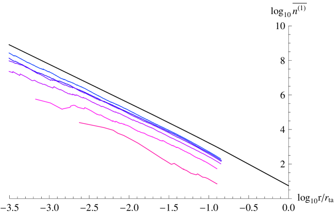
Figure 25: Mean interior energy density of loops $\log_{10}{\bar{\cal N}^{(1)}}(<r)$ (relative to unclustered loop population, including rocket effect). String tensions $G\mu=10^{-10}$ to $10^{-15}$ in powers of ten, bottom to top (colored lines) and all other parameters the same as figure 20). The black line is $\log Q_{AB}(<r)(r_{ta}/r)^{3}$ for cold dark matter. The infall model has turn-around radius $r_{ta}=1.1$ Mpc.

The enhancement of the energy density of loops as a function of galactocentric distance for a range of possible $\mu$ is summarized in figure 25. These loops are long-lived but ultimately transient residents of the galaxy. Experiments sensitive to the local Galactic population of loops, especially microlensing, will enjoy increased detection rates compared to homogeneous estimates.

Small-scale loops produced via cusps do not cluster strongly because they do not live long enough for the universe’s expansion to damp their initial relativistic motions. The galactic enhancement of loop (energy) density is $\sim 10^{-5}-10^{-4}$ that of cold dark matter depending upon the string tension ($G\mu/c^{2}<10^{-10}$) and some uncertainties in the velocity dispersion of the newly formed ultra-relativistic loops. At $10$ kpc the net enhancement of bound loops is $\mathbin{\lower 3.0pt\hbox{$\hbox to0.0pt{\raise 5.0pt\hbox{$\char 60\relax$}\hss}\mathchar 29208\relax$}}1-10$. Experiments searching for evidence of small-scale loops need to be sensitive to the homogeneous distribution throughout the universe; the local enhancement is small.

1 Introduction

Three recent developments motivate an examination of the clustering of superstring loops on galactic scales. First, braneworld cosmological scenarios that provide a framework for inflation and the big bang, necessary ingredients in modern cosmology, generically produce string-like defects. Second, string theory allows and recent investigations of warped throat compactification suggest that superstring tensions can be much smaller than the GUT scale: $G\mu/c^{2}<<10^{-6}$. Third, recent high resolution simulations of string networks suggest that $\sim 10$% of the energy available in horizon-crossing strings is transformed into loops within a few orders of magnitude of the scale of the horizon.

In the original GUT scenarios, a phase transition at the GUT energy scale created string-like defects with tension $G\mu/c^{2}\sim 10^{-6}$ whose dynamical motions generated density perturbations ultimately responsible for large scale structure formation[1, 2, 3, 4]. Intercommutation chopped long, horizon-crossing strings into loops moving at relativistic speeds. These loops, distributed in the universe in an approximately homogeneous fashion, evaporated by gravitational wave emission within a few Hubble times.

By contrast, the three advances lead to a qualitatively new and different picture for the fate of the loops. Large loop size and small string tension implies that loops survive for many expansion times. As such, they slow down by cosmic drag and fall into existing matter potential wells[5, 6].

This paper shows that low tension string loops cluster and form a halo about the Galaxy. The enhancement relative to the homogeneous loop distribution is substantial both in terms of loop numbers and loop energy (total length).

Superstring loops are roughly analogous to stellar objects in two respects: they have finite lifetimes as local luminous sources of gravitons much like nuclear burning stars emit photons over a fixed main sequence lifetime, and they are massive, compact and optically dark much like the remnants formed in post main sequence evolution. It is interesting to consider how loops, like main sequence and post main sequence stars, may reveal themselves either directly by their intrinsic emissions or indirectly by altering photon propagation of background sources. Designing and planning searches for superstring loops will require a good understanding of the distribution of loops throughout the universe and especially our own backyard.

1.1 String Tension

Inflation is an essential ingredient in modern cosmology[7, 8, 9]. In superstring theory a specific realization is brane inflation and the simplest example of brane inflation involves the interaction of a D3-brane moving toward a ${\bar{D}}3$-brane sitting at the bottom of a warped throat[10, 11, 12, 13, 14, 15, 16, 17, 18, 19, 20, 21]. The collision and annihilation of the brane pair initiates the hot big bang. Cosmic superstrings (F- and D-strings and their bound states) are produced and stretched to enormous scales[22, 23, 24, 25, 26, 27, 28, 29, 30, 31]. After the epoch of inflation these superstrings evolve by the processes of intercommutation and gravitational wave emission to yield a scaling network in which there exists a stable relative distribution of long, horizon-crossing strings and sub-horizon loops[32, 33, 34, 35, 36, 37, 38, 39, 40, 41, 42, 43, 44, 45].

The key property of a cosmic string is the tension $\mu$, or in dimensionless terms, the string’s characteristic gravitational potential $G\mu/c^{2}$. Theoretical understanding of the characteristic tension likely to emerge in a physically realistic string theory solution is far from complete. Initial estimates suggested $10^{-11}\mathbin{\lower 3.0pt\hbox{$\hbox to0.0pt{\raise 5.0pt\hbox{$\char 60\relax$}\hss}\mathchar 29208\relax$}}G\mu/c^{2}\mathbin{\lower 3.0pt\hbox{$\hbox to0.0pt{\raise 5.0pt\hbox{$\char 60\relax$}\hss}\mathchar 29208\relax$}}10^{-6}$ [28] but recent analyses of multi-brane, multi-throat scenarios have effectively removed the lower bound[24, 26, 27, 31].

Empirical upper bounds on $G\mu/c^{2}$ have been derived from null results for experiments involving lensing[46, 47, 48, 49, 50, 51, 52, 53], gravitational wave background and bursts[47, 54, 55, 56, 57, 58, 59, 60, 61, 62, 63, 64], pulsar timing[65, 47, 66, 67]and cosmic microwave background radiation[68, 69, 70, 71, 72, 73, 74, 75, 76, 77, 78, 79]. These may be generally summarized as follows: (1) Searches for signatures of optical lensing in fields of background galaxies imply $G\mu/c^{2}\mathbin{\lower 3.0pt\hbox{$\hbox to0.0pt{\raise 5.0pt\hbox{$\char 60\relax$}\hss}\mathchar 29208\relax$}}3\times 10^{-7}$. The analysis relies on the deficit angle geometry of a string in spacetime and the accurate estimation of survey selection effects. (2) Modeling of the CMB power spectrum yields $G\mu/c^{2}\mathbin{\lower 3.0pt\hbox{$\hbox to0.0pt{\raise 5.0pt\hbox{$\char 60\relax$}\hss}\mathchar 29208\relax$}}10^{-7}$. The limit is based on well-understood properties of large-scale string networks although the precise quantitative results are sensitive to unknown details of the spectra of string bound states and the probability of string-string interactions. (3) Pulsar timing stability gives $G\mu/c^{2}\mathbin{\lower 3.0pt\hbox{$\hbox to0.0pt{\raise 5.0pt\hbox{$\char 60\relax$}\hss}\mathchar 29208\relax$}}10^{-9}$. The limit assumes that loops of near-horizon scale are created by the string network.

In short, cosmic superstrings must have tensions substantially less than the original GUT-inspired strings and there is no known theoretical impediment to the magnitude of $G\mu/c^{2}$ being either comparable to or much lower than the current observational upper limits.

The lifetime $\tau$ of a loop of size $l$ to emission of gravitational radiation is, on dimensional grounds, $\tau\sim lc/(G\mu)$. Smaller tension yields larger $\tau$. In a cosmology with power law growth in the scale factor, the scaling solution chops long strings into loops of size $l\sim\alpha ct$, i.e. proportional to the size of the horizon. Here, the dimensionless constant $\alpha$ typifies a characteristic loop size from a broad, possibly multi-peaked, distribution of string loop scales. A key parameter is the number of expansion times before the loop evaporates $H\tau\sim\alpha/(G\mu/c^{2})$ where $H$ is the Hubble constant. When $H\tau$ is not big the loops evaporate before the universe has expanded significantly. Such is the case for the usual GUT-inspired structure formation scenarios.

The notions that the tension might be very small, $G\mu/c^{2}<<10^{-7}$, and that the loop size distribution include some objects comparable to the scale of the horizon ($10^{-4}<\alpha<10^{-1}$) yields qualitatively new cosmological features. If $H\tau>>1$ the resultant string network will contain many old loops. Loops born with relativistic speeds are significantly slowed by cosmic drag before evaporating. A necessary condition for clustering on a galactic scale is that the loops damp to speeds less than the typical speeds within the galaxy: $v/c<(v/c)_{gal}\sim 10^{-3}$. This is only possible for large $H\tau$.

This paper presents a detailed calculation of the infall of loops in a schematic model for growth and formation of a galactic scale cold dark matter perturbation in the presence of a scaling string network. The strings satisfy the Nambu Goto equations of motion (hereafter NG strings). The loops accumulate and form a large halo similar in many respects to the Galaxy’s gravitationally dominant dark matter halo but with several unique features: old captured loops decay by emission of gravitational radiation and are eventually ejected by the recoil associated with the anisotropy of their gravitational wave emission (“rocket effect”) while new loops are added continually near the Galaxy’s turn-around radius. At each epoch the galaxy is dressed with a long-lived halo of string loops.

§2 outlines and summarizes the various calculations and the results. Modeling details follow in subsequent sections: §3 describes the halo formation model, §4 sets up the equations of motion for string loops in inhomogeneous Friedmann-Robertson-Walker (FRW) cosmology, §5 characterizes the free motion of loops, accelerated motion and derives an approximation for the critical acceleration that unbinds a loop, §6 describes the model for the string network, §7 characterizes the clustering for string loops generated by the network at a given time, with given size, and possessing given tension, and §8 calculates the loops currently distributed within the Galaxy in two different models for loop formation.

Finally, §9 discusses some of the implications and outlines future work.

2 Executive Summary

The background cosmological model is Einstein-de Sitter with a critical density of non-relativistic matter and scale factor $a(t)\propto t^{2/3}$. The growing gravitational perturbation is much smaller in size than the horizon and treated non-relativistically. Consider the spherically symmetric infall of cold, collisionless matter caused by introducing a small overdense top hat perturbation. The turn-around radius is the point where the Hubble expansion exactly balances the infall velocity and sets the scale for the problem. Material well within the turn-around radius has had sufficient time to collapse, re-expand, recollapse, and so forth. These motions (“bounces”) rearrange the mass, kinetic energy and potential energy so as to produce a virialized structure on scales somewhat less than the turn-around radius. Material outside the turn-around radius has not yet had time to bounce. If much more material has bounced than was initially present in the top hat perturbation then the solution is self-similar, i.e. all the physical properties can be scaled from one time to another. The essential character of the self-similar infall model (i.e. the fully self-consistent density, velocity and gravitational potential of the collisionless cold dark matter which accretes and forms the non-linear bound object) has been spelled out [84, 85, 86, 87]. In this paper, the Galaxy’s growing gravitational potential is described in terms of the gravitational potential $\psi$ of the self-similar infall model.

The background metric for flat FRW is $ds^{2}=-c^{2}dt^{2}+a(t)^{2}(dx^{2}+dy^{2}+dz^{2})$. The perturbed metric is assumed to include only the scalar terms of the growing, non-relativistic gravitational potential $ds^{2}=-(1+2\psi)c^{2}dt^{2}+a(t)^{2}(1+2\Phi)(dx^{2}+dy^{2}+dz^{2})$. Anisotropies in the stress tensor are ignored; this implies $\Phi=-\psi$. There is no back-reaction of the strings on the spacetime. In the absence of gravitational wave emission, each string loop center of mass follows a geodesic in the spacetime; tidal effects on the loops are ignored.

However, the loop does emit radiation and its impulse alters the loop trajectories. Intrinsic variations in the direction of momentum radiated within the loop center of mass frame would tend to average out the net impulse given to the loop. An assumption that no torques act constitutes the “worst case” for binding of loops to the Galaxy because the direction of the rocket force is influenced only by special and general relativistic effects which are always active not by additional, intrinsic variations in the loop center of mass frame. In this paper no internal or external torques act so that the direction of the rocket impulse in the center of mass frame behaves like the spin of a particle. The impulse direction is Fermi transported along the spacetime trajectory of the loop.

The rates of gravitational wave emission of energy and momentum by oscillating loops have been previously calculated for a sparse sample of loop configurations [54, 88, 89, 90, 91, 92]. In the center of mass frame the approximate, period-averaged consequences are (1) a constant rate of change of length (or energy), $dl/dt=\Gamma_{E}(G\mu/c^{2})c$, and (2) a constant degree of anisotropy which induces an impulse $a_{r}=\Gamma_{P}(G\mu/c^{2})(c^{2}/l)$. Based on the numerical studies, typically $\Gamma_{E}\sim 50$ and $\Gamma_{P}\sim 10$ but these may vary by a factor $\sim 2$ for individual loop configurations.

In summary, a loop undergoes non-geodesic motion in spacetime because of the rocket effect with Fermi transport of the impulse direction. In the center of mass frame, the loop shrinks according to a simple, approximate description and suffers a recoil based on a fixed degree of anisotropy which determines the magnitude of the non-gravitational acceleration (hereafter “the impulse”).

When loops are chopped off from the string network they are typically moving at relativistic velocities. Initial conditions are drawn from a homogeneous distribution in space, with a relativistic center-of-mass velocity and a range of sizes. A choice of string tension $\mu$ and initial conditions for the loop (position, velocity, rocket direction and size at the time of formation $t_{i}$) yields a trajectory in the background spacetime.

The numerical results presented in this paper show how loops bind to the growing galactic perturbation. The most common scenario is that a loop born at an early time, slows down by cosmic drag, is overtaken by the turn-around radius, and accretes. The rocket effect is initially negligible. The resultant orbit is very radial passing back and forth through the galactic center with roughly fixed physical semi-major axis. Such a loop is easily identified as “bound to the perturbation.” The physical scale of the captured orbit is fixed even as the perturbation continues to grow in size. Loops captured at early times end up near the center of the structure, ones added later at the periphery.

As the loop shrinks, eventually, the acceleration of the rocket unbinds the loop from the perturbation. Detachment is rather sudden because the periodic motion in the potential averages the effect of the impulse, i.e. the orbit is adiabatically invariant. Escape follows when the rocket’s force is large enough to alter the orbital parameters within a single orbit.

The general trends can be understood by reference to the behavior of cold dark matter. Cold dark matter falls into the growing perturbation and creates a well-defined, universal profile with scale set by the turn-around radius. The cumulative probability distribution for a cold dark matter particle to be bound to the perturbation is a function of a single dimensionless parameter, the ratio of radius to turn-around radius. The analogous distribution for bound loops is more complicated since it depends on the epoch of formation, the size of the loop, and the string tension.

Loops – formed at early epochs but with small enough $\mu$ that they have not yet neared the end of their lives – behave just like cold dark matter. They assume the same universal profile near the center while at large galactic radii the profile is truncated due to the rocket effect (“outer cutoff”).

Dynamical complications ensue for loops formed at much earlier or much later times. For old loops that have begun to shrink substantially the importance of the rocket effect increases; consequently, the outer cutoff in the Galactic profile of loops becomes more important, i.e. it moves inward. Every loop is unbound before it completely evaporates because in that limit the acceleration from the rocket grows large. New loops, on the other hand, which are typically born with relativistic speeds have not yet damped sufficiently to allow capture by the potential. A set of graphs illustrate the constraints on formation size, formation time and string tension.

An integration over the rate of creation of loops implied by recent network simulations of Nambu Goto strings yields an estimate of today’s loop profile about the Galactic center. The main part of the bound population was created by fragmentation of horizon-scale strings into large sub-horizon loops. The loops are abundant and overdense with respect to the universe’s average number and energy density of strings of all sorts.

The bottom line results for large loops are presented in figures 24 (number density of loops within the galaxy relative to the homogeneous value) and 25 (energy density of loops relative to homogeneous value). These figures show a substantial degree of enhancement in both measures that depends upon string tension and spans a large interval of galactocentric radii. Such profiles motivate more accurate calculations for gravitational wave, pulsar timing and microlensing experiments hunting for evidence of loops within the Galaxy.

The radial distribution of loops within the Galaxy is weighted to the center. The size distribution of loops is weighted to small scales with a cutoff corresponding to a loop with evaporation lifetime equal to the age of the universe.

By contrast, cusp-generated small loops fail to bind to the Galaxy. This is not surprising given their ultra-relativistic initial motions and their reduced lifetimes. The bottom line results for small loops are presented in figures 29 (number density) and 30 (energy density). Little enhancement is observed within the range of radii at which the radial infall model is applicable.

These results are broadly suggestive that clustering of large loops will play an important role in setting microlensing rates and may also increase the effective sensitivity of gravitational wave and pulsar timing experiments. On the other hand, experiments sensitive to small loops will not benefit from significant local enhancement.

3 Halo Formation Model

3.1 Aim

The role of the halo formation model in this paper is to provide a dynamical background for the motion and eventual capture of the string loops generated by the network. The density and potential of the cold dark matter are determined in a self-consistent fashion and the string loops moved as test particles in the potential. The distribution of cold dark matter particles and string loops can then be compared.

3.2 Self-similar Radial Infall

Refs. [84], [85], [86], and [87] have analyzed the spherically symmetric infall of cold, collisionless matter onto small-scale density enhancements in an Einstein-de Sitter universe. The solution is self-similar i.e. the form and appearance at any time is fixed when scaled to a characteristic physical length. The infall yields power law halo density distribution $\rho\propto r^{-2.25}$ and rotation curves $\propto r^{-1/8}$. The model is physically self-consistent and simple enough that many difficult aspects of the cosmology plus network evolution can be handled precisely.

The model solution is exact given the assumptions but the model must be regarded as a schematic description of the Galaxy. Its basic shortcomings in comparison to a realistic treatment of $\Lambda$CDM cosmology are the following: (1) it ignores the initial spectrum of perturbations which span a great range of length scales and it suppresses the generic asymmetry of a typical perturbation that grows to encompass a galaxy scale mass, (2) it is only applicable at times after equipartition and before late-time acceleration.

Of these, the more significant issue is the first. Initial conditions drawn from a CDM spectrum generate a hierarchy of mergers not a monolithic infall[94, 95, 96, 97]. Today objects like our Galaxy have dark matter density profiles that are non-power law [98]. The density $\rho$ varies like $1/r$ at small radii (successive mergers of small dense objects) and $1/r^{3}$ at large radii (truncation of infall). The radial infall model does not capture the behavior at either extreme: it should be adequate on scales on which the rotation curve is observed to be flat, $3<r<30$ kpc, and it may be adequate out to distances where the curve is traditionally assumed or inferred to be flat, e.g. $\sim 100$ kpc[99]. The motivation for its use here is that a comparison of the loop and cold dark matter distributions calculated in the same, self-consistent time-dependent potential, should yield valid conclusions of greater generality than might be suggested by a strict comparison of actual to modeled Galactic profiles.

Of course, $a\propto t^{1/2}$ prior to the time of equipartition $t_{eq}$ and the perturbation begins to grow only for $t>t_{eq}$. It is incorrect to use the self-similar form for the potential at early times. Nonetheless, this paper employs it focusing on clustering after equipartition. Since the dynamics of loops formed before equipartition are an essential part of the story to be set forth one might worry that this presents an additional important shortcoming. In the current model, the turn-around radius at $t_{eq}$ is $\sim 15$ pc; the radial profile of cold dark matter and of loops at such small scales would certainly be inaccurately represented even if the perturbation were exactly spherical. (Which it is not – as already indicated the smallest radius at which the radial infall model applies is much larger.) On larger scales the distribution of cold dark matter and loops is not adversely impacted since the potential is basically flat while cosmic drag and the rocket effect both operate independently of the potential. A loop slows down first and then binds to the growing perturbation when the turn-around radius reaches it. This typically occurs at $t>t_{eq}$. At times $t>t_{eq}$, the cold dark matter density and gravitational potential quickly asymptote to the self-similar form. Computed properties today are uninfluenced.

Finally, the late-time acceleration of the universe alters the behavior of the turn-around radius. This certainly changes how loops might be added to the outermost periphery of the Galaxy. Since M31 will turn out to be closer than turn-around radius formally inferred today, it is clear that quantitative agreement at such large distances is not expected.

Future work will treat structure growth in realistic simulations of the $\Lambda$CDM paradigm.

3.3 Model Specifics

This exposition follows the mathematical description given by Ref. [87]. At time $t_{i}$ consider a small top hat density enhancement $\delta_{i}\equiv(\delta\rho/\rho_{H})_{i}$ which extends from the origin to physical radius $R_{i}$; assume the Hubble constant $H_{i}$ is independent of radius. All the material in the universe is bound by the presence of the excess material and is destined to fall towards it.

The motion of shells depends upon the initial position $r_{i}$, the initial velocity $r_{i}H_{i}$ and the mass interior to the shell. Write the initial mean density within a radius $r_{i}$ in terms of ${\bar{\Omega}}_{i}=1+\Delta_{i}$ where $\Delta_{i}=\delta_{i}\min\left(1,\left(\frac{R_{i}}{r_{i}}\right)^{3}\right)$. Before a shell crosses any other shell, it satisfies the parametric equations

$$r = \frac{r_{i}{\bar{\Omega}}_{i}}{2\left({\bar{\Omega}}_{i}-1\right)}\left(1-\cos\theta\right)$$ (1)

$$t = \frac{{\bar{\Omega}}_{i}}{2H_{i}\left({\bar{\Omega}}_{i}-1\right)^{3/2}}\left(\theta-\sin\theta\right).$$ (2)

The initial state at $t=0$ has parameter $\theta=0$. To lowest order in $\Delta_{i}<<1$ it turns around ($\theta=\pi$) at

$$r_{ta} = \frac{r_{i}}{\Delta_{i}}$$ (3)

$$t_{ta} = \frac{\pi}{2H_{i}\Delta_{i}^{3/2}}.$$ (4)

Eliminating the occurrences of $r_{i}$ in favor of $\delta_{i}^{1/3}R_{i}$ yields the turn-around radius at any given time $t$ as

$$r_{ta}=\delta_{i}^{1/3}R_{i}\left(\frac{2H_{i}t}{\pi}\right)^{8/9}.$$ (5)

The fact that $r_{ta}$ involves the product of a single combination of variables and the characteristic power law $t^{8/9}$ is a significant simplification. The turn-around radius is a suitable length scale with which to non-dimensionalize the problem. The dimensionless length scale $\lambda$ is a pure function of the parameter $\theta$:

$$\lambda = \frac{r(t)}{r_{ta}(t)}=\frac{\sin^{2}\left(\frac{\theta}{2}\right)}{\left(\frac{\theta-\sin\theta}{\pi}\right)^{8/9}}.$$ (6)

A shell starting at a large distance from the top hat has large $\lambda$. As the turn-around radius increases and the shell falls under the influence of the perturbation $\lambda$ decreases.

The initial motion is orderly. Before shell-crossing occurs the dimensionless velocity ${\cal V}$, dimensionless mass ${\cal M}$ and dimensionless density ${\hat{\rho}}$ are explicit functions of $\theta$:

$${\cal V} = \frac{\dot{r}}{\left(\frac{a_{ta}(t)}{t}\right)}=\frac{\pi^{8/9}}{2}\frac{\sin\theta}{1-\cos\theta}\left(\theta-\sin\theta\right)^{1/9}$$ (7)

$${\cal M} = \frac{3M}{4\pi\rho_{H}(t)r_{ta}(t)^{3}}=\frac{9\lambda^{3}}{16}\frac{\left(\theta-\sin\theta\right)^{2}}{\sin^{6}\left(\frac{\theta}{2}\right)}$$ (8)

$${\hat{\rho}} = \frac{\rho}{\rho_{H}(t)}=\frac{1}{1+3\chi}\frac{\left(\frac{3}{4}\left(\theta-\sin\theta\right)\right)^{2}}{\sin^{6}\left(\frac{\theta}{2}\right)}$$ (9)

$$\chi = 1-\frac{3V}{2\lambda}$$ (10)

and $\rho_{H}(t)$ is the density of the background model.

The initial state corresponds to $\theta\to 0$; the asymptotic forms in this limit are

$$\lambda \to \frac{\left(6\pi\right)^{8/9}}{4\theta^{2/3}}$$ (11)

$${\cal V} \to \frac{2\lambda}{3}$$ (12)

$${\cal M} \to \lambda^{3}$$ (13)

$${\cal\rho} \to 1.$$ (14)

The excess mass associated with the perturbation

$${\cal M}_{x} = \lambda^{3}\left(\frac{9}{16}\frac{\left(\theta-\sin\theta\right)^{2}}{\sin^{6}\left(\frac{\theta}{2}\right)}-1\right)$$ (15)

is used to infer the potential that will make its appearance in the metric in the next section.

Eventually, the infalling shell meets shells that have already bounced. The first crossing for a shell occurs at $\lambda_{1}=0.364$. The dimensionless expressions above are exact for $\lambda>\lambda_{1}$. Once crossings begin for the shell of interest, the mass interior to it varies and must be calculated to find the acceleration and trajectory. Ref. [87] has solved the problem numerically and tabulated ${\cal M}(\lambda)$ for $0.02<\lambda<\lambda_{1}$ and also provided a power law approximation for $\lambda<<1$. This paper uses a combination of asymptotic, tabulated and analytic expressions to describe ${\cal M}(\lambda)$ and ${\cal M}_{x}(\lambda)$ over the complete range of $\lambda$. The dimensionless cumulative mass is shown in figure 1.

The dimensionless radial component for the force and potential are deduced from ${\cal M}_{x}$:

$${\cal F} = \frac{f}{\frac{4\pi}{3}G\rho(t)r_{ta}(t)}=-\frac{M_{x}}{\lambda^{2}}$$ (16)

$${\hat{\psi}} = \frac{\psi}{\frac{4\pi}{3}G\rho(t)r_{ta}^{2}}=-\int_{r/r_{ta}}^{\infty}\frac{M_{x}}{\lambda^{2}}d\lambda.$$ (17)

The fact that the force and potential, which are intrinsically functions of four spacetime variables, are compactly represented in terms of the one-dimensional functions of the dimensionless radius $\lambda=r/r_{ta}(t)$ is a great simplification. Test particle motion in the vicinity of the perturbation depends upon the these functions. The dimensionless potential is shown in figure 2.

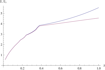
Figure 1: The cumulative mass bound to the perturbation as a function of distance from the center; $\lambda=r/r_{ta}$ is the scaled radial coordinate; the mass is expressed in units of $4\pi\rho(t)r_{ta}^{3}/3$ where $\rho(t)$ is the background (critical) density. The curve is continuous with changes in slope (density discontinuities) at shell-crossings. The upper curve is the entire mass including that contributed by the mean background; the lower curve is the excess with respect to the background.

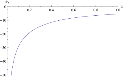
Figure 2: The gravitational potential associated with the excess mass as a function of distance from the center; $\psi_{x}$ is the gravitational potential measured in units of $4\pi G\rho(t)r_{ta}^{2}/3$ (with value zero at spatial infinity) and $\lambda=r/r_{ta}$.

To apply the infall model to the Galaxy today the turn-around radius must be specified. Assume that the well-virialized part of the halo has a physical scale today $R_{g}=150$ kpc. The current age is fixed at the concordance value $t_{0}=1.37\times 10^{10}$ yrs [100]. Let the epoch for the turn-around of the material at $R_{g}$ be $t_{1}$ and let the turn-around radius at that time be $r_{ta,1}$. Figure 3 illustrates the history of a particle as it passes back and forth through the center. Its apocenter approaches an asymptotic value of $\sim 0.8r_{ta,1}$. Between 4 and 5 passages, the apocenter has shrunk from $r_{ta,1}$ at time $t_{1}$ to $0.845r_{ta,1}$ at time $8t_{1}$. With some arbitrariness, identify $R_{g}=0.845r_{ta,1}$ and $t_{0}\sim 8t_{1}$. Since $r_{ta}\propto t^{8/9}$ this implies the turn-around radius today is $r_{ta,0}=1.1$ Mpc.

All the quantitative properties of the self-similar description now follow. Assuming that radial infall continues to the present, at the Sun’s galactocentric radius today ($8.5$ kpc) the rotation velocity is $225$ km s^-1 and the interior mass is $10^{11}{\rm M}_{\odot}$. The model has total mass $7.5\times 10^{11}{\rm M}_{\odot}$ within $R_{g}$ today. Turnaround at $t_{1}/t_{0}\sim 0.12$ occurs before the switch from power law to exponential expansion in the concordance $\Lambda$CDM model ($t_{\Lambda}/t_{0}\sim 0.73$) so the late-time deviations from Einstein-de Sitter should be relatively unimportant. If infall were to cease at $t>t_{1}$ the net change in mass within the solar circle is estimated to be $\sim 4$% and within $R_{g}$ to be $\sim 40$%.

This completes the specification of the time-dependent Galactic model.

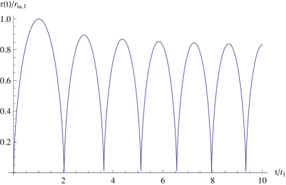
Figure 3: The motion of a single particle in the collisionless infall solution. Time is in units of the initial turn-around time $t_{1}$, physical radius in units of the initial turn-around radius $r_{ta,1}$. The curve is a fit to numerical results (Table 6 in [87]).

4 Equations of Motion in Inhomogeneous FRW Cosmology

The unperturbed background model is flat Friedmann-Robertson-Walker (FRW). Consider a frame in which the universe appears isotropic and let $x^{\alpha}=(t,x^{i})$ where $t$ is the global time coordinate and $x^{i}$ are the global comoving spatial coordinates. The scale factor is $a(t)$. Henceforth, adopt units with $c=1$.

The FRW metric with scalar perturbations is

$$g_{\mu\nu}=\left(\begin{array}[]{cccc}-(1+2\psi)&&&\\ &a^{2}(1+2\Phi)&&\\ &&a^{2}(1+2\Phi)&\\ &&&a^{2}(1+2\Phi)\end{array}\right)$$ (18)

where $\psi(x^{\alpha})$ and $\Phi(x^{\alpha})$ represent the effect of inhomogeneities. Bound structures have $\psi<0$.

The perturbation potentials are very non-relativistic (rotation velocity $\sim 225$ km/s for our Galaxy implies $v\sim 10^{-3}$). The Galaxy is assumed to be at rest in the preferred FRW frame. Only small errors are made by equating the local time and space coordinates introduced in the previous section to the global FRW coordinates ($t,ax^{i}$). Assume also $\Phi=-\psi$ which is suitable for small quadrupolar components to the stress energy tensor for the cold dark matter particles.

In the FRW frame, let a loop’s velocity be $V^{\alpha}$. If there were no rocket effect the loop would follow a geodesic through spacetime (ignoring tidal effects). However, the loop does emit radiation and its impulse alters the loop trajectory. Let the rocket’s 4-impulse be $a_{r}N^{\alpha}$ where $a_{r}$ is the time-varying magnitude of the impulse.

Consider, first, the direction of the rocket’s impulse. In the center of mass frame, (1) loops formed in cosmological fragmentation scenarios generally possess net angular momentum[101], (2) the angular momentum radiated over an oscillation period lies parallel to the angular momentum of the loop[81], and (3) the momentum radiated over an oscillation period lies in a direction generally different than that of the angular momentum of the loop. Item (2) implies that loops spin down in a relatively simple manner, however, item (3) suggests that the net gravitational force does not act on the center of mass of the loop. The emission of angular momentum has been studied only for loops of the simplest complexity. Though there is no evidence to date, more complex loops might experience more complex dynamics.

Ref. [80] treats the loop as a relativistic gyroscope and concludes from a dimensional argument that the timescale for a single precession cycle is $\sim\tau$, i.e. comparable to the loop lifetime. Since the momentum impulse is not along the angular momentum direction this argument suggests but does not prove that the rocket direction is fixed for the life of the loop. On the other hand, if one treats the loop as a solid body [81] the precession time is considerably shorter $\sim\sqrt{G\mu/c^{2}}\tau$. A suitable gravitational wave back-reaction calculation that would definitively address how the direction of momentum impulse varies is unavailable ([102] did not investigate precession and [103] studied a symmetric loop that did not radiate momentum).

Intrinsic variations of the rocket direction in the loop center of mass frame would tend to average out the net impulse given to the loop. A fixed direction gives the “most effective” rocket and presents the “worst case” for binding of loops to the Galaxy.

Assume (1) the impulse in the loop center of mass frame lies along a fixed direction and (2) no torques act in the loop center of mass frame. Then $N^{\alpha}$ is simply the Fermi-transported impulse direction of the loop. The normalizations are $V^{\alpha}V_{\alpha}=-1$ and $N^{\alpha}N_{\alpha}=1$ and orthogonality is $N^{\alpha}V_{\alpha}=0$. The equations of motion are

$$\frac{dV^{\alpha}}{d\tau}+\Gamma^{\alpha}_{\beta\gamma}V^{\beta}V^{\gamma} = a_{r}N^{\alpha}$$ (19)

$$\frac{dN^{\alpha}}{d\tau}+\Gamma^{\alpha}_{\beta\gamma}N^{\beta}V^{\gamma} = a_{r}V^{\alpha}$$ (20)

for proper time $\tau$. For the numerical solution in the FRW frame, the 4-vectors for velocity and for the internally generated impulse direction are parameterized

$$V^{\mu} = \left(\frac{\sqrt{1+v^{2}}}{\sqrt{1+2\psi}},\frac{v{\hat{v}}^{i}}{a\sqrt{1+2\Phi}}\right)$$ (21)

$$N^{\mu} = \left(\pm\frac{\sqrt{n^{2}-1}}{\sqrt{1+2\psi}},\frac{n{\hat{n}}^{i}}{a\sqrt{1+2\Phi}}\right)$$ (22)

where $v^{2}=g_{ij}V^{i}V^{j}$, $n^{2}=g_{ij}N^{i}N^{j}$, and ${\hat{v}}^{i}$ and ${\hat{n}}^{i}$ are 3D-orthonormal unit vectors (${\hat{v}}\cdot{\hat{v}}\equiv\sum_{i}{\hat{v}}^{i}{\hat{v}}^{i}=1$ and ${\hat{n}}\cdot{\hat{n}}=1$). The equations for $dx^{i}/dt$, $dv/dt$, $d{\hat{v}}/dt$, $dn/dt$ and $d{\hat{n}}/dt$ are expressed using the global FRW time as the independent coordinate. These equations are applicable to loops with the whole range of possible velocities from extremely relativistic to non-relativistic. The explicit form is given in the Appendix A.

Let the total loop energy be $E$ in the FRW frame and, following custom, denote $E/\mu$ as length $l$. For clarity, explicitly label quantities in the string’s center of mass frame with “z”. The infinitesimal length (i.e. energy) is $dl_{(z)}=d\sigma\sqrt{(d{\vec{z}}/d\sigma)^{2}/(1-{\dot{\vec{z}}}^{2})}$ where ${\vec{z}}={\vec{z}}(\sigma,z^{0})$ is the parametric expression for the string; $l=V^{0}l_{(z)}$ and $dt=V^{0}dz^{0}$.

In the loop center of mass frame the rate of energy loss and the magnitude of the impulse are very simple

$$\frac{dl_{(z)}}{dz^{0}} = -\Gamma_{E}G\mu$$ (23)

$$a_{r} = \Gamma_{P}\frac{G\mu}{l_{(z)}}.$$ (24)

The loop lifetime is a fixed increment of time in the center of mass frame. The 4-impulse in the center of mass frame is $a_{(z)}^{\alpha}=(0,a_{(z)}^{i})=a_{r}(0,n_{(z)}^{i})$ where $n_{(z)}^{i}$ is a unit vector in the direction of the impulse and $a_{r}$ is the magnitude of the impulse. Since $a_{r}$ is a scalar, $a^{\alpha}a_{\alpha}=a_{(z)}^{\alpha}a_{(z)\alpha}=a_{r}^{2}$, write the 4-impulse $a_{r}N^{\alpha}$ in the FRW frame. Since the initial loop configuration ${\vec{z}}(\sigma,z^{0})$ determines $n_{(z)}^{i}$ and no torques operate (by assumption) it is most convenient to find the initial $N^{\alpha}$ in FRW frame (Appendix B) and use Fermi transport to determine its subsequent evolution in that frame.

In the FRW frame

$$\frac{dl}{dt} = \frac{l}{V^{0}}\frac{dV^{0}}{dt}-\Gamma_{E}G\mu$$ (25)

$$\frac{d}{dt}\left(\frac{1}{a_{r}}\right) = -\frac{\Gamma_{E}}{\Gamma_{P}V^{0}}.$$ (26)

After $a_{r}N^{\alpha}$ is initially set the entire calculation can be carried out in the FRW frame using Fermi transport for $N^{\alpha}$ and the above equation for $a_{r}$.

There are a variety of non-trivial frame transformation effects that operate in this schematic description of loop evolution. Ignoring the momentum impulse of the rocket and the inhomogeneous potential, in the FRW frame a loop born with length $l_{i}$ with center of mass motion $V^{0}_{i}=\sqrt{1+v_{i}^{2}}$ at time $t_{i}$ has length and center of mass momentum

$$l = \sqrt{\frac{1+v^{2}}{1+v_{i}^{2}}}\left(l_{i}-t_{i}\frac{\Gamma_{E}G\mu}{\nu}\sqrt{1+v_{i}^{2}}\int_{1}^{a/a_{i}}\frac{x^{1/\nu}dx}{\sqrt{x^{2}+v_{i}^{2}}}\right)$$ (27)

$$v = \frac{v_{i}a_{i}}{a}$$ (28)

at scale factor $a=a_{i}(t/t_{i})^{\nu}$. The initial loop size that just evaporates at scale $a/a_{i}$ is explicitly given by setting the expression within the parenthesis to 0. It is clear that complete evaporation occurs in a finite FRW time.

The time a loop lives is slightly different than the above result in a homogeneous universe because of the ever increasing importance of the rocket effect. The loop length still vanishes in a finite time. Let the time until evaporation be $\Delta t=t_{life}-t$ and the ratio of momentum-to-energy loss $\beta=\Gamma_{P}/\Gamma_{E}$. Then the length, acceleration and momentum parameter vary asymptotically

$$l \propto \Delta t$$ (29)

$$a_{r} \propto \Delta t^{-1/(1-\beta)}$$ (30)

$$v \propto \Delta t^{-\beta/(1-\beta)}$$ (31)

The difference between the approximate and exact lifetimes is only $\sim 2.3$% ($\Gamma_{E}=50$, $\Gamma_{P}=10$, $v_{i}=0.1$) which will be ignored in subsequent discussion. The acceleration and the momentum-per-mass both diverge as the evaporation proceeds to completion.

5 Characterization of Orbits

5.1 Radial Geodesics

The first calculations illustrate some basic kinematic features for objects whose initial velocity is very different from Hubble flow. Consider purely radial geodesics and ignore the rocket effect. Fix the magnitude of the initial radial velocity to be $v_{i}=0.1$ (typical of the largest loops chopped off from the horizon crossing strings) at the initial time $t_{i}/t_{0}=10^{-9}$. The results that follow are for the full, relativistic equations of motion. One calculation differs from another only in terms of the initial position of the loop with respect to the spherical center.

Figure 4 shows the comoving trajectories of a set of loops as a function of $\log t/t_{0}$. The different colors label different initial positions and ingoing and outgoing velocities. The velocity $v$ is damped by the many decades of expansion (in the absence of a varying potential $v(t)\sim v_{i}a_{i}/a(t)$), a fact made qualitatively clear from the flattening of all the curves at early times. Once a loop’s motion has been damped, it behaves for all practical purposes like a cold dark matter particle at the position to which it has moved. The comoving coordinate is nearly but not exactly static because every zero-velocity object is bound to the excess central mass of the perturbation. In the absence of the rocket effect, each loop eventually turns around, the comoving coordinate retreats and the loop oscillates back and forth through the perturbation center. To avoid clutter, only the first few bounces of each loop are plotted. The color of the line allows tracing the epoch of turn-around and recollapse for a loop to a given initial position. The black line is the comoving turn-around radius in the radial infall model.

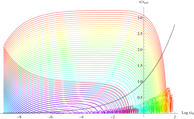
Figure 4: Comoving position as a function of $\log t/t_{0}$. Radial geodesics (no rocket effect) have been integrated from a set of initial positions with fixed initial radial velocity $v_{i}=0.1$ (either inward or outward) at time $t_{i}/t_{0}=10^{-9}$. Distance is measured in units of today’s comoving turn-around distance. The black line shows the comoving turn-around radius.

Figures 5 and 6 are blow ups in comoving and physical coordinates respectively for $10^{-3}<t/t_{0}<1$. They show the first few bounces after capture of the loops by the perturbation. These figures as well as the previous one demonstrate that early (late) turn-around implies small (large) semi-major axes just as is true for the cold dark matter particles in the radial infall model. Figure 5 illustrates that loops starting in different regions of space with different initial velocities (red and blue lines) can end up with nearly identical accretion orbits. This is simply the shuffling in position that occurs during the time it takes for cosmic drag to operate. As a side note, the absence of red lines is a consequence of the limited range of initial radii sampled; had larger offsets been plotted such lines would be present throughout the figure. Figure 6 makes it clear that there exist loops that “turn around” at the same space time locations as cold dark matter particles do.

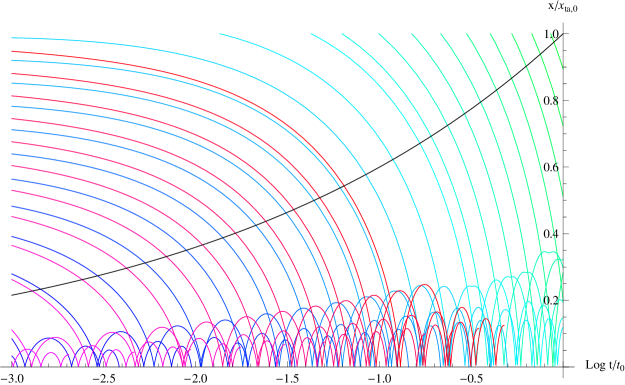
Figure 5: Detailed view of the trajectories in figure 4. The different colored lines indicate different initial conditions. Only the first few bounces through the center are plotted. Consequently, the increase in amplitude with time highlights a sequence of loops falling into the perturbation having systematically larger orbits not that an individual loop’s bounces grow in amplitude.

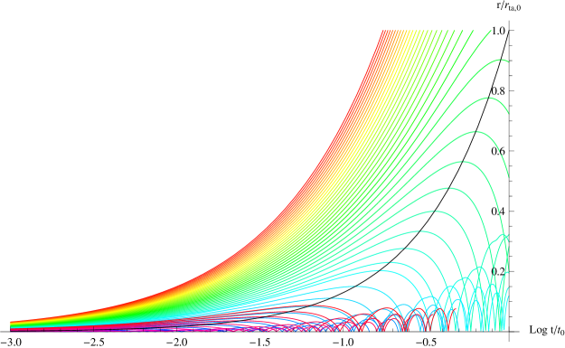
Figure 6: Detailed view of physical separation for trajectories in figure 4. Only the first few bounces through the center are plotted. In physical coordinates, the bounces occur with nearly fixed amplitude. Same comments as for figure 5 apply.

If a loop is young then cosmic expansion may not have had sufficient opportunity to damp its velocity to allow accretion onto the growing perturbation at a physical radius of interest. A simple estimate of how small $t_{i}/t_{0}$ must be for a loop to capture at time $t$ is given as follows. Cosmic drag implies the initial velocity decays like $v(t)=v_{i}a_{i}/a(t)$ (flat potentials). A necessary condition for capture is that $v(t)$ must be less than the escape velocity from the potential. However, a generally more restrictive condition is that capture requires $v(t)<H(t)r_{ta}(t)$. Since the turn-around radius $r_{ta}(t)=r_{ta}(t_{0})\left(\frac{t}{t_{0}}\right)^{8/9}$ the initial time is constrained to be $t_{i}/t_{0}<\left(\frac{H_{0}r_{ta}(t_{0})}{v_{i}}\right)^{3/2}\left(\frac{t}{t_{0}}\right)^{5/6}$. For example, a loop with initial velocity $v_{i}=0.1$ can be captured today if $t_{i}/t_{0}\mathbin{\lower 3.0pt\hbox{$\hbox to0.0pt{\raise 5.0pt\hbox{$\char 60\relax$}\hss}\mathchar 29208\relax$}}7.5\times 10^{-5}$ and will have a physical orbit $\sim r_{ta}(t_{0})$. Physical radius and time of capture are inherently linked in the similarity solution. A loop with physical orbit $r<r_{ta}(t_{0})$ must be accreted at earlier time $t/t_{0}=(r/r_{ta}(t_{0}))^{9/8}$; the initial time of formation of that loop is constrained to be $t_{i}/t_{0}<\left(\frac{H_{0}r_{ta}(t_{0})}{v_{i}}\right)^{3/2}\left(\frac{r}{r_{ta}(t_{0})}\right)^{15/16}$. For example, for $r=30$ kpc, sufficient cosmic drag requires the loop be formed at $t_{i}/t_{0}<2.5\times 10^{-6}$ and captured at $t/t_{0}\sim 1.7\times 10^{-2}$.

Figure 7 shows the comoving trajectories of a set of loops born at $t_{i}/t_{0}=10^{-4}$ (the ordinate is greatly expanded compared to previous figures). The slope for orbits far away from the perturbation indicates that cosmic drag has not yet brought the loops to rest. This impedes capture. Figure 8, a detailed view near the origin, shows that when it does occur it does so at large physical separation.

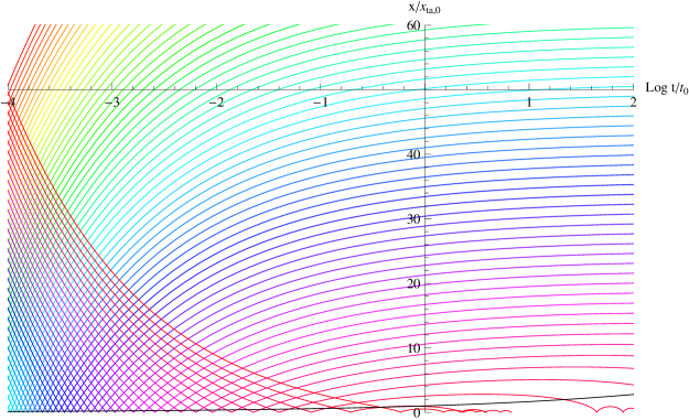
Figure 7: Same as figure 4 but with $t_{i}/t_{0}=10^{-4}$.

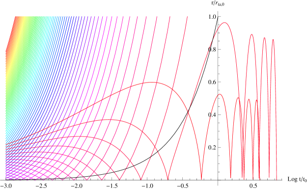
Figure 8: Same as figure 7 but in physical coordinates.

5.2 Rocket Effect

The rocket effect can inhibit binding of a loop to the growing perturbation and can unbind a previously captured loop. This section begins with analytic estimates and follows with full numerical calculations.

Begin by considering homogeneous FRW with rocket direction aligned or anti-aligned with initial velocity. The equations of motion (Appendix A) reduce to

$$\frac{dv}{dt} = \delta\frac{na_{r}}{\sqrt{1+v^{2}}}-v\frac{\dot{a}}{a}$$ (32)

$$\frac{dn}{dt} = \delta\frac{va_{r}}{\sqrt{1+v^{2}}}-\frac{nv^{2}{\dot{a}}}{a(1+v^{2})}$$ (33)

$$\frac{da_{r}}{dt} = \frac{\Gamma_{E}a_{r}^{2}}{\Gamma_{P}\sqrt{1+v^{2}}}$$ (34)

$$\delta = {\hat{n}}\cdot{\hat{v}}=\pm 1$$ (35)

with initial velocity $v_{i}$ and loop length $l_{i}=\alpha/H_{i}=(3/2)\alpha t_{i}$ in the matter-dominated, FRW frame at time $t_{i}$. The initial rocket impulse is $a_{r,i}=\Gamma_{P}G\mu\sqrt{1+v_{i}^{2}}/l_{i}$ and the FRW direction vector is $n_{i}=\sqrt{1+v_{i}^{2}}$. The equation for $n$ may be solved and its occurrences eliminated. For non-relativistic motions, the equation for $a_{r}$ may also be integrated explicitly to give

$$\frac{dv}{dt} = \delta\frac{\Gamma_{P}}{\Gamma_{E}}\frac{1}{\tau_{i}+t_{i}-t}-v\frac{\dot{a}}{a}$$ (36)

$$\tau_{i} = \frac{l_{i}}{\Gamma_{E}G\mu}$$ (37)

Here $\tau_{i}$ is the characteristic time for the loop to evaporate by gravitational wave radiation. If $\tau_{i}+t_{i}>>t$ then the first term is approximately constant and $v$ is a sum of terms proportional to $t$ and $t^{-2/3}$ [54, 83]. The limit of interest is $H\tau>>1$. Specifically, if $\kappa^{-1}\equiv(5\Gamma_{E}/(2\Gamma_{P}))v_{i}H_{i}\tau_{i}=(5\alpha v_{i}/(2\Gamma_{P}G\mu))>>1$ then

$$v\simeq v_{i}\left(\left(\frac{t_{i}}{t}\right)^{2/3}+\delta\frac{\kappa t}{t_{i}}\right)$$ (38)

Capture at radius $r$ of the accelerated trajectory for a loop with aligned velocity and rocket impulse ($\delta=1$) requires

$$\kappa<\frac{\frac{H_{0}r_{ta,0}}{v_{i}}\left(\frac{t_{0}}{t_{i}}\right)^{2/3}\left(\frac{r}{r_{ta,0}}\right)^{5/8}-1}{\left(\frac{r}{r_{ta,0}}\right)^{15/8}\left(\frac{t_{0}}{t_{i}}\right)^{5/3}}$$ (39)

by the same line of argument given in the previous section. The numerator must be positive and implies an upper limit on the time of formation

$$\left(\frac{H_{0}r_{ta,0}}{v_{i}}\right)^{3/2}\left(\frac{r}{r_{ta,0}}\right)^{15/16}>\frac{t_{i}}{t_{0}}$$ (40)

identical to that in the previous section. This is the effect of cosmic drag and does not depend upon $\mu$. For loops formed at earlier times, capture requires

$$G\mu<\frac{5\alpha}{2\Gamma_{P}}H_{0}r_{ta,0}\left(\frac{r_{ta,0}}{r}\right)^{5/4}\frac{t_{i}}{t_{0}}$$ (41)

a result that highlights the importance of the rocket effect.

The condition that the loop not evaporate by the current epoch requires

$$G\mu<\frac{3\alpha}{2\Gamma_{E}}\frac{t_{i}}{t_{0}}.$$ (42)

For a given epoch of formation, the upper limit on tension is rocket-related for $r/r_{ta,0}>(5\Gamma_{E}/(3\Gamma_{P}))^{4/5}(H_{0}r_{ta,0})^{4/5}\sim 7.6\times 10^{-3}$ or $r\mathbin{\lower 3.0pt\hbox{$\hbox to0.0pt{\raise 5.0pt\hbox{$\char 62\relax$}\hss}\mathchar 29208\relax$}}8.5$ kpc and age-related at smaller radii.

The maximum tension that permits capture (the intersection of limits implied by equations 40 and 41 or 42; this is the rightmost section of the triangular region formed by green and turquoise lines in figure 9 ) is

$$G\mu|_{critical} = \frac{5\alpha}{2\Gamma_{P}}v_{i}\left(\frac{H_{0}r_{ta,0}}{v_{i}}\right)^{5/2}\left(\frac{r_{ta,0}}{r}\right)^{5/16}{\rm min}\left(1,\frac{3\Gamma_{P}}{5\Gamma_{E}}\left(H_{0}r_{ta,0}\right)^{-1}\left(\frac{r}{r_{ta,0}}\right)^{5/4}\right)$$ (43)

$$= 4.12\times 10^{-9}\left(\frac{\alpha}{0.1}\right)\left(\frac{0.1}{v_{i}}\right)^{3/2}\left(\frac{10{\rm kpc}}{r}\right)^{5/16}{\rm min}\left(1,\left(\frac{r}{8.5{\rm kpc}}\right)^{5/4}\right)$$ (44)

Above this critical $G\mu/c^{2}$, loops do not cluster at scale $r$ within the Galaxy. Curiously, the critical $G\mu$ has a maximum close to the Sun’s galactocentric position though the variation from $r=3-100$ kpc is only about $2.7$ (and with all other parameters fixed).

All captured loops are eventually stripped from the galaxy by the rocket effect. A detailed discussion of how removal proceeds is given in the next section. The result is that $a_{r}>0.3|\nabla\psi|$ leads to detachment. For fixed loop size, a loop is retained until the current epoch if

$$G\mu<\frac{0.15\alpha}{\Gamma_{P}}H_{0}r_{ta,0}\frac{{\cal M}_{x}}{\lambda^{2}}\frac{t_{i}}{t_{0}}$$ (45)

For small $\lambda$ the asymptotic form for the mass distribution is ${\cal M}_{x}\sim 10.5\lambda^{3/4}$, so that ${\cal M}_{x}/\lambda^{2}\propto\lambda^{-5/4}$ just as in eq. 41. This retention criterion is very similar to the capture criterion but quantitatively a bit stricter (the constant for retention is $\sim 0.6$ that of the capture). However, the physical interpretations are very different. Capture is a statement about the properties of the loop and turn-around radius at early times whereas retention concerns all later times up to the current epoch. Because of the self-similar evolution of the perturbation both criteria vary with $t_{0}$ identically for fixed loop size. As the loop shrinks, the retention criterion becomes more and more strict. In summary, the retention criterion is only a bit stricter for fixed loop size but becomes far stricter once the loop size begins to change.

Figure 9 provides a graphical summary of some of the analytic results and a point of reference throughout this section which describes additional calculations.

The above analysis is now supplemented by a study of the rocket’s effect on loop dynamics via a sequence of trajectory calculations of increasing complexity. The numerical investigation proceeds along the following lines. First, locate the specific radial trajectories that give rise to orbits of fixed physical size today for $\mu=0$, i.e. without the accelerative force. Second, starting from the inferred initial conditions, repeat the calculation of the trajectories including the effect of gravitational wave recoil. The rocket effect is slight at first but dominates by the end of the loop lifetime. Comparison of different $\mu$ yields a criterion for retaining a loop at the radius of interest today. Figure 9 includes some of the numerical results.

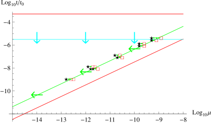
Figure 9: Bounds on formation time and string tension for a loop with initial velocity $v_{i}=0.1$ to be captured at physical radius $30$ kpc. (1) Upper bounds on the formation time $t_{i}/t_{0}$ are given by the horizontal lines. The condition that cosmic drag lower the velocity to less than the circular rotation velocity today is given by the red line. The more stringent condition that capture occur at $30$ kpc is given by the turquoise line. (2) Upper bounds on the string tension $G\mu/c^{2}$ are given by the diagonal lines. The initial loop size is $\alpha/H_{i}$ and $\alpha=0.1$. The condition that the loop be younger than its gravitational wave decay timescale is given by the red line. The more stringent condition that the loop not be accelerated out of the Galaxy is given by the green line ($\chi>\chi_{crit}$). The geometric symbols summarize results from numerical experiments examining the outcome today ($t=t_{0}$) for groups of 10-20 loops captured at $30$ kpc with slightly different string tensions: stars = all loops bound, boxes = all loops ejected, triangles = some bound and some ejected (for clarity the points are slightly offset in the vertical but not the horizontal direction). (3) The triangular region encompasses string tensions and formation times giving bound loops at $30$ kpc for $v_{i}=0.1$ and $\alpha=0.1$ in a radial infall model of the Galaxy. The critical value of $\mu$ below which clustering is possible is determined by the upper right hand corner of the green and turquoise lines. Lowering $v_{i}$ raises the limit on $t_{i}/t_{0}$ (horizontal lines moves upward); lowering $\alpha$ shifts the bound to smaller $\mu$ (diagonal lines moves leftward). Shifting the loop orbital scale to smaller values (say the solar position) requires earlier formation times (horizontal lines shifts down) and allows larger $\mu$ (green line shifts to the right but is limited by the red line which is fixed).

Begin by choosing a time for the birth of the loop $t_{i}/t_{0}$ ($10^{-9}$ to $1$) and fixing the initial radial velocity ($v_{i}=0.1$). Then find the initial position that ends with an orbit of the desired apocenter at the current epoch (two specific cases, $10$ and $30$ kpc, are considered; the apocenter is estimated based on the last 2 extrema of the orbit prior to $t_{0}$). This is a boundary value problem for the equations of motion and is solved by numerical iteration.

For each case, two qualitatively distinct orbital solutions for small $t_{i}$ were found; no attempt was made to find all solutions. As $t_{i}$ increased the initial conditions for the individual solutions converged and for $t$ greater than a critical value no suitable initial conditions could be found. This result is consistent with the order-of-magnitude argument given above. The variation of the initial position with $t_{i}/t_{0}$ of the two branches is systematic and shown in figure 10.

Both branches of $30$ kpc orbits are over plotted in comoving coordinates in 11; they begin at different times and different velocities but note that all converge to similar oscillatory solutions. These solutions are the “baseline” solutions which are now perturbed by the rocket effect.

Figure 10: Initial comoving coordinate positions (ordinate) at a set of different formation epochs (abscissa) for loops that evolve to give orbits of fixed physical size today. The green (blue) points are the initial conditions that give 30 (10) kpc orbits. The two branches are two qualitatively different solutions to the boundary value problem described in the text. The loop in the lower branch passes through the perturbation center, slows down and is overtaken by the turn-around radius. The one in the upper branch begins moving outward and is overtaken by the turn-around radius.

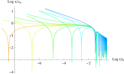
Figure 11: The different lines illustrate the comoving radial coordinate of loops formed at different times and yielding $30$ kpc orbits today. These are the explicit solutions to the boundary-value problem whose initial conditions are displayed in Figure 10; they correspond to the green upper and lower branches.

Starting from the initial conditions inferred above, repeat the calculations with non-zero $\mu$ and a set of random orientations for the rocket in the loop center of mass frame. Varying $\mu$ delimits the transition from bound to unbound orbits at the current epoch. Small (large) $\mu$ implies weak (strong) acceleration. The transition refers to a specific time, $t=t_{0}$, as it is clear that eventually, for long enough integrations, the orbits of all evaporating loops are unbound.

The initial position and velocity in figures 12-14 are all identical, i.e. that of a loop born at $t_{i}/t_{0}=10^{-9}$ which formed a bound $30$ kpc orbits in the absence of the rocket effect. A sequence of calculations with increasing $\log_{10}\mu=-12.8$, $-12.7$ and $-12.6$ and random rocket orientations unbinds an increasing fraction of orbits. Each figure includes the original unperturbed orbit for comparison.

Besides the fact that the transition occurs over a fairly narrow range in $\mu$, the figures also illustrate that the apocenter does not significantly change until just before the orbit is actually destroyed.

Figure 12: Initial time $t_{i}/t_{0}=10^{-9}$, initial velocity $v_{i}=0.1$, $\mu=10^{-12.8}$. Eight trajectories with randomly chosen initial momentum directions and the original unperturbed trajectory (golden yellow color) are plotted

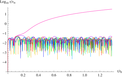
Figure 13: Same as 12 but $\mu=10^{-12.7}$. One trajectory is detached.

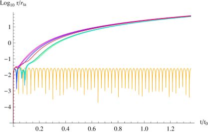
Figure 14: Same as 12 but $\mu=10^{-12.6}$. All the perturbed trajectories escape. About half the trajectories are captured and later detached while the rest avoid capture completely. The unperturbed trajectory is golden yellow.

A summary of the results for a range of $\mu$ and $t_{i}/t_{0}$ for bound $30$ kpc orbits appears in figure 9. The geometric symbols characterize the outcomes for groups of orbits: stars, boxes and triangles mean “all bound”, “all ejected” and “a mixture” of both types, respectively. The green diagonal line is an analytic estimate for the critical $\mu$ based on non-relativistic calculations in the following section which imply that a loop is detached when the magnitude of its rocket impulse $a_{r}$ satisfies $a_{r}\mathbin{\lower 3.0pt\hbox{$\hbox to0.0pt{\raise 5.0pt\hbox{$\char 62\relax$}\hss}\mathchar 29208\relax$}}0.3|\nabla\psi|$. The transition from bound to unbound is abrupt (a factor of $2$ in $\mu$ encompasses its entire scope) stemming from the adiabatic invariance associated with averaging weak forces over periodic orbits.

This figure summarizes the main physical constraints for binding and residency of loops in the Galactic halo. There are upper bounds on the formation time $t_{i}/t_{0}$ given by the horizontal lines. The condition that cosmic drag lower the velocity to less than the circular rotation velocity is given by the red line. The more stringent condition that capture occur is given by the turquoise line. There are upper bounds on the string tension given by the diagonal lines. The condition that the loop be younger than its gravitational wave decay timescale is given by the red line. The more stringent condition that the loop not be accelerated out of the Galaxy is given by the green line. The critical $G\mu/c^{2}$ below which capture and retention is possible is given by the intersection of the green and turquoise lines. Appendix C includes a graph which replaces the straight lines with numerically determined conditions for aligned and anti-aligned rocket orientations.

The triangular region encompasses string tensions and formation times for loops that are bound to our Galaxy today. The specifics of this figure refer to loops at radius $30$ kpc, with initial velocity $v_{i}=0.1$, and initial length $\alpha/H_{i}$ where $\alpha=0.1$ in a radial infall model of the Galaxy. The manner in which the constraints vary is briefly discussed in the caption.

5.3 Critical Acceleration

It is well known from classical mechanics that the action of a simple harmonic oscillator with frequency $\omega$ is an adiabatic invariant. Perturbative driving forces having intrinsic frequency $\Omega$ such that $\Omega<<\omega$ produce exponentially small changes in the action or energy. Here, perturbative means that the magnitude of the forcing is small, i.e. the instantaneous change to the coordinate is first order. The integrated change of a first order quantity over a full period is very small.

The rocket acts on the loop’s orbit within the Galaxy. For loops which have slowed enough to bind to the Galaxy, the Fermi transport of the impulse direction (an analog of Thomas spin precession) has frequency $\Omega\sim v^{2}\omega\sim 10^{-6}\omega$. Effectively, the acceleration is in a fixed direction with magnitude $a_{r}$ governed by the decrease in length of the loop. The condition for escape is equivalent to the breakdown in adiabatic invariance of the oscillator that occurs when the force grows sufficiently large to become non-perturbative.

The main complication for an actual orbit is that the potential is not separable and several incommensurate $\omega$’s exist (radial and angular frequencies), so that one cannot solely focus on the motion in the coordinate direction defined by the impulse. However, it is straightforward to investigate a simple, non-relativistic model having all the essential features and to infer an approximate criterion for the transition from perturbative to non-perturbative motion. Consider an acceleration law of the form

$${\vec{a}}=\frac{-{\vec{r}}}{\left(r^{2}+r_{c}^{2}\right)^{\frac{n+1}{2}}}+{\vec{k}}.$$ (46)

The interpretation here is that the first term is the acceleration due to the galactic matter distribution and the second term is the internal acceleration due to the rocket. The constants are core radius $r_{c}$, internal acceleration $\vec{k}$ and galactic acceleration power law $n$. For a Keplerian potential $n=2$, for the radial infall model $n=5/4$ and for galactic potentials the range of interest is $1<n<2$. To non-dimensionalize, express lengths in units of $r_{c}$.

For a numerical investigation, first choose the initial radial displacement of a zero-velocity particle and the size of the internal acceleration, and sample random choices of direction $\hat{k}$. The unperturbed orbit would remain radial if not for the internal acceleration which drives it away from that limit. Define $\chi\equiv|k|(r^{2}+r_{c}^{2})^{n/2}$ as a measure of the ratio of internal to galactic forces and evaluate it along the unperturbed trajectory. Next, integrate the actual orbit to determine whether it remains bound to the center. After many samplings of $\hat{k}$, one calculates $f_{bind}(\chi)$ the fraction of bound particles at a fixed value of $\chi$.

Repeating this procedure for different initial positions ($5$-$20r_{c}$) and power law shapes ($n=1$-$2$) allows comparison of the importance of the various inputs to the calculation. Figure 15 displays $f_{bind}(\chi)$ for different $n$. For a fixed $n$, the geometric orientation of the rocket produces an intrinsic spread in outcomes for $0.2\mathbin{\lower 3.0pt\hbox{$\hbox to0.0pt{\raise 5.0pt\hbox{$\char 60\relax$}\hss}\mathchar 29208\relax$}}\chi\mathbin{\lower 3.0pt\hbox{$\hbox to0.0pt{\raise 5.0pt\hbox{$\char 60\relax$}\hss}\mathchar 29208\relax$}}0.8$. By comparison, the entire range of $n$ corresponds to relatively small shifts in $\chi$. This geometric effect is large and irreducible compared to the uncertainties in the initial position, power law shape and number of orbital periods.

To help gauge the importance of internal forces on the binding of orbits, it is useful to define the critical ratio of internal to galactic forces by $f_{bind}(\chi_{crit})=1/2$. While there is some variation, $\chi_{crit}\sim 0.3$ is a reasonable estimate. In applying this result to the loop dynamics evaluate $\chi=a_{r}/|\nabla\psi|$ at apocenter and regard the orbit as unbound if $\chi>\chi_{crit}$.

These results have been used to speed up the large-scale numerical calculations determining the probability of capture and the halo profiles in the sections that follow. Essentially, the rocket effect is ignored before capture and the retention and lifetime criteria at the epoch of interest are imposed to determine the bound population of living loops. Since the retention criterion is generally stricter than the capture criterion little error is made and this allows a single simulation to be used for multiple values of $G\mu$.

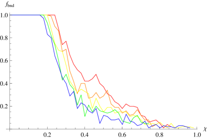
Figure 15: The fraction of radial orbits that remain bound as a function of $\chi$ for power law exponents $n=1$, $5/4$, $3/2$, $7/4$ and $2$ (red, orange, yellow, green and blue, respectively). All orbits began at an apocenter of $20$ core radii; 100 random orientations for the internal acceleration were drawn; for each choice the orbit was integrated many characteristic orbital times; the curves summarize the bound fraction.

6 Network Evolution

The halo will contain loops born with a variety of positions, velocities, times of formation and lengths. This section discusses the birth rate density for loops generated by a scaling network. Succeeding sections discuss the average probability of capture for loops created at a given epoch and the net effect when the birth rate density is integrated over all length and time scales.

6.1 Status of Large and Small Loops

Early simulations of Nambu Goto strings[32, 35, 104, 105, 33]successfully tackled the large scale properties of the network, in particular, the relation of horizon to correlation length, characteristic spacing and persistence length. They validated the original idea that the network would evolve to reach a scaling solution in simulations[106]. The attraction of arbitrary initial conditions to a scaling solution insures that the energy density in long, horizon-crossing strings never comes to dominate the total energy density of the universe. This is a necessary but not sufficient condition to avoid overclosing the universe since loops formed during the radiation era must decay by some mechanism to avoid a monopole-like problem. For strings that couple only to the gravitational field the decay must involve gravitational wave emission.

Loops are created when the horizon crossing strings are chopped up. It was originally thought that loops would form by intercommutations of the long strings at the characteristic scale of the horizon (the Kibble one-scale model). Since the early studies found clear signs of a gas of small loops and dense kink-filled string segments at the simulations’ resolution limit it became apparent that some basic understanding had yet to be achieved. In a perfect scaling solution all the properties of the network, not just those close to that of the horizon, should scale. Characterizing the small scale structure and searching for evidence of its scaling has been an ongoing effort.

The significance of the small scale structure has now become more apparent. It turns out that rather than being a detail to be disentangled from resolution issues, the small scale structure is inextricably intertwined with the evolution of the network on all scales less than the horizon. Small scale structure governs many potentially observable features of the network and ultimately has a considerable impact on the expected halo clustering properties of loops. This section briefly reviews areas of significance for the problem of loop clustering.

Current numerical simulations of NG strings generate a continuum distribution of sub-horizon scale loops including some loops that are much bigger than the resolution limit[37, 40, 107]. Although non-trivial differences exist between the most recent simulations a point of common agreement is that the abundance of loops near the horizon scale is greater than found in the earlier, lower resolution work. Roughly $\sim 10$% of the length of long strings ends up in loops with length $10^{-4}<l/t<10^{-1}$. For the purposes of this paper, these are all “large” loops because they imply $H\tau>>1$ for $G\mu/c^{2}<<10^{-7}$. A second area of mutual agreement is that the population of these large loops is judged to be scaling and is not a transient artifact. The presence of a population of large loops hearkens back to the original expectation that the horizon scale would determine the properties of newly formed loops.

The traditional interpretation of the large loop part of the distribution is that it forms via a sequence of multiple encounters in which a horizon-scale loop is cut into smaller and smaller progeny. Some of these encounters are with the long, horizon crossing component, some with other loops and some are self-intersections in which a loop oscillates so that individual parts collide. Ref [37] indicates that self-intersection of larger loops is the dominant overall loop production mechanism. An assessment of the clustering of such loops is carried out in this paper.

Both new and old simulations also contain large numbers of small loops. Early calculations suggested [108, 109] and recent studies have demonstrated that tiny loops are produced in great abundance by the interaction of small scale structure on string segments as those segments first form a large scale cusp [38, 36]. The small scale structure today owes its existence to non-linear interactions that the string experienced in the past at the time it first entered the horizon. Ref. [38] quantified the structure in terms of a correlator $\propto(l/t)^{2\chi}$ for size scale $l$ at time $t$ and showed that $\chi$ is completely determined by mean network properties (rate of expansion of the universe and rms velocity of the strings). The slope of the spatial correlation function of simulations agrees well with the theoretically-determined $\chi$ over the expected range.

Most loops (measured in terms of number or total length) are created at small physical scale with a cutoff set by gravitational damping and theoretically derived to be $\alpha\sim(G\mu/c^{2})^{1+2\chi}$ where $\chi=0.1$ or $0.25$ for radiation or matter respectively[110, 111, 39]. Numerical simulations do not include gravitational wave damping so it isn’t possible to verify directly the cutoff prediction. However, the slope of the loop size distribution depends upon $\chi$, is insensitive above the cutoff to the actual value of the cutoff and agrees well with that found in simulation[36].

It appears that roughly 90% of the horizon crossing string goes into tiny loops [112, 113]. There are many factors which will end up influencing the clustering of small loops. While there are more small loops than large ones, small loops evaporate more quickly than large ones. Loops at the gravitational wave cutoff are ultra-relativistic [38]. Time-dilation and cosmic expansion effects (eq. 27) in the ultra-relativistic limit imply $H\tau\sim\left(\alpha c^{2}/G\mu\right)^{1/(1+\nu)}\sim\left(G\mu/c^{2}\right)^{2\chi/(1+\nu)}$. In the matter era, $\nu=2/3$, $\chi=0.25$ so $H\tau\sim(G\mu/c^{2})^{0.3}$; in the radiation era, $\nu=1/2$, $\chi=0.1$ and $H\tau\sim(G\mu/c^{2})^{0.13}$. All these results suggest that loops at the cutoff may be unable to cluster but the small power of $G\mu/c^{2}$ means $H\tau$ is never very small and the significance of loops larger than the cutoff (which live longer) is murky. The multiplicity of factors at play suggests that a detailed calculation of clustering should be carried out.

6.2 Birth Rate Density

The long horizon crossing strings are chopped into loops at a rate

$$\left(\frac{d\rho}{dt}\right)_{\infty\to{\rm loops}}=\frac{2\rho_{\infty}}{t}\left(1-\nu\left(1+{\bar{v}}_{\infty}^{2}\right)\right)$$ (47)

where $\rho_{\infty}=\mu/(\gamma_{s}t)^{2}$ is the energy density in long strings with typical separation $\gamma_{s}t$ and mean square velocity ${\bar{v}}_{\infty}^{2}$ [114].

As long as a scaling solution is achieved when horizon $\propto t$ (true for power law expansion in radiation and matter dominated eras but not applicable to the recent $\Lambda$-dominated phase) then the average birth rate of loops of physical size $l$ per physical volume $V$ at time $t$

$$\frac{dN}{dldtdV}=\frac{f(x)}{t^{5}}$$ (48)

where $x=l/t=\alpha/(Ht)$ for some function $f(x)$.

The loop formation process involves interactions within the network and, simultaneously, stretching of the horizon crossing strings and expansion of the universe. At least a few expansion times ($\sim 1/H$) are needed for intercommutations to transform long string segments into sub-horizon loops. Once sub horizon loops are formed the probability for loop-loop interactions decreases and the loop achieves a fixed physical size in a few more expansion times. The assumption in this paper is that during each infinitesimal time interval $(t,t+dt)$ the network produces the loops implied by $dN/dldtdV$. The loops have physical scale that changes only due to gravitational radiation; they suffer no further intercommutation. This prescription provides the distribution of initial conditions for the clustering calculation.

In principle, the full joint distribution of $dN/dldtdV$, loop center of mass momentum and rocket direction in the center of mass frame is needed to realize the initial conditions for the dynamical motion of a population of loops in the background FRW cosmology. In lieu of a detailed description, assume a factorized form for the joint distribution

$$\frac{dN}{dldtdVd{\vec{v}}d{\hat{\Omega}_{r}}} = \frac{dN}{dldtdV}\frac{dP}{d{\vec{v}}}\frac{dP}{d{\hat{\Omega}_{r}}}$$ (49)

where $\vec{v}$ is the loop center of mass momentum and ${\hat{\Omega}}_{r}$ the direction of the rocket. Here, $dP/d(..)$ means the differential probability for the initial condition of $(..)$ with unit normalization. In practice, the correlations between the magnitude of the momentum $v$ and $l/t$ is retained but all correlations between the direction of the momentum, the direction of the impulse and $l/t$ are discarded.

In the homogeneous limit number $N$ and length $L$ of loops created in comoving volume $\tilde{V}=V_{0}/a_{0}^{3}$ (i.e. the comoving volume implied by a physical volume $V_{0}$ today; $a_{0}=a(t_{0})$) are

$$\left(\begin{array}[]{c}N\\ L\end{array}\right)=\frac{V_{0}}{t_{0}^{3}}\int\frac{dy^{\prime}}{y^{\prime 4}}\left(\frac{a^{\prime}}{a_{0}}\right)^{3}\int dx^{\prime}\left(\begin{array}[]{c}f(x^{\prime})\\ f(x^{\prime})x^{\prime}\end{array}\right)$$ (50)

where $y=t/t_{0}$, $x=l/t$ and $a^{\prime}=a(t^{\prime})$. By the current time some loops have evaporated and all have shorter lengths. The distribution of loops with length is

$$\frac{dN_{A}}{dl}=\frac{V_{0}}{t_{0}^{3}}\int\frac{dy^{\prime}}{y^{\prime 4}}\left(\frac{a^{\prime}}{a_{0}}\right)^{3}\int dx^{\prime}f(x^{\prime})\int d{\vec{v}}^{\prime}d{\Omega_{{\hat{r}}^{\prime}}}\frac{dP}{d{\vec{v}}^{\prime}}\frac{dP}{d{\Omega_{{\hat{r}}^{\prime}}}}\delta\left(l-L\right)\theta_{A}$$ (51)

where $L=L[{\vec{v}}^{\prime},l^{\prime},{\Omega_{{\hat{r}}^{\prime}}},t^{\prime};t_{0}]$ is length at $t_{0}$ in terms of the initial loop parameters and, similarly, $\Theta_{A}=\Theta_{A}[{\vec{v}}^{\prime},l^{\prime},{\Omega_{{\hat{r}}^{\prime}}},t^{\prime};t_{0}]$ is 0 or 1 depending upon whether the loop has reached the end of its life or not. The dependence of $L$ and $\Theta_{A}$ on dynamical variables may be traced to relativistic effects that link FRW and loop center of mass frames. Quantities $N_{A}$ and $L_{A}$ are defined by integrals over $dN_{A}/dl$.

When the loop’s center of mass motion is only mildly relativistic then the loop lives until $t_{life}=t^{\prime}+l^{\prime}/(G\mu\Gamma_{E})$. Hence $\Theta_{A}=1$ for $t<t_{life}$ and the loop length is $L=l^{\prime}-\Gamma_{E}G\mu(t-t^{\prime})$ independent of the loop dynamics. To summarize: for non-relativistic kinematics and ignoring the dynamical influence of the rocket the forms for $L$ and $\Theta_{A}$ simplify: $L=L[l^{\prime},t^{\prime};t_{0}]$ and $\Theta_{A}=\Theta_{A}[l^{\prime},t^{\prime};t_{0}]$ giving

$$\frac{dN_{A}}{dl}=\frac{V_{0}}{t_{0}^{3}}\int\frac{dy^{\prime}}{y^{\prime 4}}\left(\frac{a^{\prime}}{a_{0}}\right)^{3}\int dx^{\prime}f(x^{\prime})\delta\left(l-L\right)\theta_{A}.$$ (52)

The integration over $x^{\prime}=l^{\prime}/t^{\prime}$ follows directly since occurrences of $l^{\prime}$ are now easily rewritten in terms of $l$, $t_{0}$ and $t^{\prime}$.

6.3 Fragmentation and Cusp-Mediated Loop Formation

Until this point, the network evolution has been treated in an agnostic fashion with respect to the scaling solutions for matter and radiation eras. For the purposes of presenting numerical results, the focus tightens to matter era network evolution. This choice avoids any potential inconsistency with respect to the growing galactic perturbation for which matter era dynamics are most appropriate. It also simplifies and streamlines the presentation. However, most loops in the halo today were born before equipartition and the absolute numbers of such loops depend upon the radiation era expansion dynamics [5]. This paper concentrates on enhancement, i.e. the ratio of clustered to homogeneously distributed loops which is expected to be less sensitive to expansion dynamics.

Large loops are created by hierarchical fragmentation; small loops by cusps interacting with pre-existing small scale structure. The processes are both active at the same time. The description for each mechanism begins with the power law form

$$f(x)=\left\{\begin{array}[]{cc}Ax^{-\beta}&{\rm~{}if}~{}~{}x_{L}<x<x_{U}\\ 0&{\rm else}\end{array}\right.$$ (53)

which depends upon $A$, $\beta$, $x_{L}$ and $x_{U}$. Individual $f$’s for individual mechanisms are weighted by the fraction $\delta$ of the total energy loss rate by horizon crossing string $(d\rho/dt)_{\infty\to{\rm loops}}$ that ends up in loops created by a given mechanism. Energy balance gives

$$A=\delta\frac{2(2-\beta)}{\gamma_{s}^{2}\left(x_{U}^{2-\beta}-x_{L}^{2-\beta}\right)}\left(1-\nu\left(1+{\bar{v}}^{2}_{\infty}\right)\right)$$ (54)

In the non-relativistic matter era, $\nu=2/3$, $\gamma_{s}^{2}=10^{-1}$ and ${\bar{v}}^{2}_{\infty}=0.35$.

Refs. [38, 36] explored the cusp-mediated mechanism and combined theoretical arguments and simulation-derived average quantities to infer in the matter era

$$\chi = 0.25$$ (55)

$$\beta = 3-2\chi$$ (56)

$$x_{L} = \frac{l_{gw}}{t}=20.\left(G\mu\right)^{1+2\chi}.$$ (57)

For the cusp-mediated mechanism $f$ is strongly tilted to small scales; the upper cutoff $x_{U}$ has little effect. Ref. [38] derived the means square velocity distribution for newly formed loops

$$\langle\beta^{2}\rangle=1-\frac{2B}{(2\chi+1)(2\chi+2)}\left(\frac{l}{t}\right)^{2\chi}$$ (58)

where $B=0.61$.

In this paper, the theoretically derived $f$ is adopted to describe cusp-mediated loop production. The cutoff $x_{U}$ is adjusted freely. Ref. [38] noted that a puzzling discrepancy exists between the above expression for $\langle\beta^{2}\rangle$ and previous, simulation-derived dispersions [115] with the theoretical result being larger. Since loops with higher velocity must experience more damping before they are able to cluster adopting the theoretical expression gives the “worst case” scenario for small loop clustering. The implications of a reduced $\langle\beta^{2}\rangle$ will be investigated as well.

Ideally a similar approach for the hierarchical formation mechanism should be followed. Fits for $f$ for large loops in an expanding cosmology are not generally available and a systematic comparison of existing simulation results is lacking. One network simulation [107] gave a scaling, unimodal distribution at $x\sim 0.1$ for $f$ but another [40] lacked the peak and generated an approximate power law form for $f$ at smaller $x$.

A potential practical complication is the extent the cusp-mediated contribution interferes in fits to $f$ designed to characterize the fragmentation mechanism. Figure 3 in [36] showed that cusp-mediated loop production traces $x^{2}f(x)$ from the simulation [107] over the range $x<10^{-2}$. This subsumes a significant part of the loop range termed “large” here.

In sum, the form for $f$ for the fragmentation mechanism for large loops has not yet been sufficiently well-characterized to yield specific values for $\delta$, $\beta$, $x_{L}$ and $x_{U}$. The values of $\delta$ and $x_{U}$ are the most important and the most uncertain input for many purposes.

In this paper $\delta$, $\beta$, $x_{L}$ and $x_{U}$ are regarded as free parameters for assessing the impact on loop clustering. Simulation-based results for $\langle\beta^{2}\rangle$ as a function of $l/t$ [115] were fit using the same form as eq. 58 in a purely empirical manner. In the matter era the results are $B=1.46$ and $\chi=0.114$. This fit for large loops formed by fragmentation will also be employed as an alternative to the theoretically derived $\langle\beta^{2}\rangle$ for small loop motions.

For all mechanisms, the loop momentum distribution ($v$) is assumed to be thermal in the FRW frame, i.e.

$$\frac{dP}{d{\vec{v}}} = \frac{dP}{dv}\frac{dP}{d\Omega_{\hat{v}}}$$ (59)

$$\frac{dP}{dv} = \frac{v^{2}e^{-\kappa E}}{\int dv^{\prime}v^{\prime 2}e^{-\kappa E^{\prime}}}$$ (60)

$$E(v) = \sqrt{1+v^{2}}$$ (61)

$$\frac{dP}{d\Omega_{\hat{v}}} = \frac{1}{4\pi}$$ (62)

where $\kappa=\kappa(x)$ is set by requiring agreement with the fits to the dispersion $\left<\beta^{2}\right>$.

The direction of rocket impulse is assumed to be isotropic in the loop center of mass frame.

7 Loop Clustering

This section describes the halo profile formed by loops which are born at a single epoch and with a fixed $l/t$.

7.1 Probability of Capture

Consider the probability that a single loop formed at time $t_{i}$ in a large but arbitrary comoving volume $\tilde{V}$ ends up today bound to the galaxy with physical semi-major axis $r$. Let $\Delta N$ be the number of loops formed in infinitesimal time interval $t^{\prime}$ to $t^{\prime}+dt^{\prime}$ for $t^{\prime}=t_{i}$.

First, write out the formal probability that the loop has not evaporated and is bound with position $\vec{x}$, momentum $\vec{v}$ and length $l$ today

$$\frac{dP_{AB}}{d{\vec{x}}d{\vec{v}}d{l}} = \frac{\frac{d}{d{\vec{x}}d{\vec{v}}d{l}}{\Delta N_{AB}}}{\Delta N}$$ (63)

$$= \frac{1}{\tilde{V}}\int d{\vec{x}^{\prime}}d{\vec{v}^{\prime}}d{\Omega_{{\hat{r}}^{\prime}}}\frac{dP}{dl^{\prime}}\frac{dP}{d\vec{v}^{\prime}}\frac{dP}{d\Omega_{{\hat{r}}^{\prime}}}\delta^{3}({\vec{x}}-{\vec{X}})\delta^{3}({\vec{v}}-{\vec{V}})\delta(l-L)\theta_{AB}$$ (64)

$$\frac{dP}{dl^{\prime}} = \frac{f}{\int fdl}=\frac{f}{t^{\prime}F}$$ (65)

$$F = \int f(x)dx$$ (66)

The initial variables are position ${\vec{x}^{\prime}}$ (assumed homogeneous), velocity ${\vec{v}^{\prime}}$, length $l^{\prime}$. Here ${\vec{X}}={\vec{X}}({\vec{x}^{\prime}},{\vec{v}^{\prime}},l^{\prime},{\Omega_{{\hat{r}}^{\prime}}},t^{\prime};t_{0})$ is the formal time-dependent solution for position, likewise for ${\vec{V}}$ and $L$. The function $\theta_{AB}$ is 1 if the loop is alive (has not yet evaporated) and bound to the perturbation and 0 otherwise. The probability that the loop has initial length $l^{\prime}$ is $dP/dl^{\prime}$ and similarly for the other initial variables. Here, $F$ is a normalization constant.

Evaluate this integral by Monte-Carlo methods for $t^{\prime}=t_{i}$: first, sample $l^{\prime}$, ${\vec{x}}^{\prime}$ and ${\vec{v}}^{\prime}$ and then use direct numerical integration to evaluate the final positions and momenta. Finally, marginalize the multi-dimensional distribution and focus solely on semi-major axes $r$ and current loop length $l$:

$$\frac{dP_{AB}}{drdl} = \int d{\vec{x}}d{\vec{v}}\frac{dP_{AB}}{d{\vec{x}}d{\vec{v}}d{l}}\delta(r-R)$$ (67)

$$\frac{dP_{AB}}{dr} = \int dl\frac{dP_{AB}}{drdl}$$ (68)

where $R=R({\vec{x}},{\vec{v}},t_{0})$ is the formal expression for the semi-major axis in terms of the current phase space coordinates. A more detailed description is given in Appendix D.

The total probability the loop is bound today is proportional to $1/\tilde{V}$. As a basis for comparison, consider the case of a cold dark matter particle: it is judged to be bound if it lies within today’s comoving turn-around volume $\tilde{V}_{ta}$. Scale the differential and cumulative forms by the same factor:

$$\frac{dQ_{AB}}{dr} = \frac{\tilde{V}}{\tilde{V}_{ta}}\frac{dP_{AB}}{dr}$$ (69)

$$Q_{AB}(<r) = \int_{0}^{r}\frac{dQ_{AB}}{dr}dr$$ (70)

The combination $nV_{ta}Q_{AB}(<r)$ is the expected number of bound objects today within distance $r$ for a mean homogeneous density $n$ and turn-around volume $V_{ta}$. By construction, cold dark matter has $Q_{AB}(<r_{ta})={\cal M}(\lambda=1)=9\pi^{2}/16=5.55$. The fact that $Q_{AB}(<r_{ta})>1$ shows that the perturbation attracts distant particles so that the total within today’s comoving turn-around volume is larger than the number in an equivalent volume far from the perturbation center.

The mean interior density is

$${\bar{n}_{AB}}=\frac{Q_{AB}(<r)}{\lambda^{3}}$$ (71)

also a useful measure of the clustering and highlights the part of the distribution near the center.

7.2 Halo Profiles

Integrating from $t^{\prime}=t_{i}$ to the present gives the expected differential number of loops in comoving volume $\tilde{V}=V_{0}/a_{0}^{3}$ today

$$\frac{dN_{AB}}{d{\vec{x}}d{\vec{v}}dl} = V_{0}F\int\frac{dt^{\prime}}{(t^{\prime})^{4}}\left(\frac{a^{\prime}}{a_{0}}\right)^{3}\frac{dP_{AB}}{d{\vec{x}}d{\vec{v}}dl}$$ (72)

$$= V_{ta}F\int\frac{dt^{\prime}}{(t^{\prime})^{4}}\left(\frac{a^{\prime}}{a_{0}}\right)^{3}\frac{dQ_{AB}}{d{\vec{x}}d{\vec{v}}dl}$$ (73)

$$\frac{dN_{AB}}{drdl} = V_{ta}F\int\frac{dt^{\prime}}{(t^{\prime})^{4}}\left(\frac{a^{\prime}}{a_{0}}\right)^{3}\frac{dQ_{AB}}{drdl}$$ (74)

The differential probabilities include a factor $1/Ft^{\prime}$.

Objects must not have fully evaporated ($\Theta_{A}=1$) and must be bound ($\Theta_{B}=1$) to the perturbation to contribute to these distributions. The length is integrated as a variable so its straightforward to evaluate $\Theta_{A}$. In practice, deciding whether a loop is bound amounts to checking whether the orbit has experienced multiple passages through the perturbation center (capture). If captured, the integration is suspended but it must still be determined when the rocket effect detaches it. If the loop is captured and not detached at the epoch of interest it is called bound.

7.3 Truncation by Rocket

A loop remains bound with approximately fixed semi-major axis until the internal acceleration exceeds that due to the gravitational potential. The condition for escape is $\chi>\chi_{crit}$ at which point the loop leaves quickly on an orbital timescale.

When the rocket is ignored, the geodesic trajectory is independent of $l$ and $\mu$ i.e. just the motion of a test object. As the loop shrinks, the rocket acceleration grows monotonically $\propto\mu/l$ while the acceleration at apocenter for a captured loop is constant. Consequently, eventually $\chi>\chi_{crit}$. For loops with non-relativistic velocities

$$\chi = \frac{a_{R}}{a}$$ (75)

$$a_{R} = \Gamma_{P}\frac{G\mu}{l}=\frac{\Gamma_{P}}{\Gamma_{E}}\frac{1}{t_{life}-t}$$ (76)

$$a = \frac{GM_{x}}{r_{ap}^{2}}=\frac{4\pi}{3}G\rho_{H}(t_{0})r_{ta}\frac{{\cal M}_{x}}{\lambda^{2}}$$ (77)

where $r_{ap}$ is the physical apocenter, the loop lives until $t_{life}=t+l/(G\mu\Gamma_{E})$ and $\lambda={r_{ap}}/{r_{ta}}$. In practice, $t$, $r_{ap}$ and $l$ are determined at the instant the loop is judged as bound so that the non-relativistic approximation is good.

The acceleration $a\propto{\cal M}_{x}/\lambda^{2}$ is monotonically decreasing with $\lambda$ or $r_{ap}$. For bound loops with given $t_{life}$ (i.e. time of formation, size and tension) there is a single value for $r_{ap}$ today which satisfies $\chi=\chi_{crit}$. Denote the solution $r_{ap,cr}(t^{\prime},l^{\prime},\mu)$.

Assume an ejected loop instantaneously leaves the galaxy. Loops with $r_{ap}>r_{ap,cr}$ have been lost; loops with $r_{ap}<r_{ap,cr}$ are still in the halo. To summarize: $\Theta_{B}$ contains a factor $\Theta\left(r_{ap}<r_{ap,cr}\right)$ which accounts for loop loss by the rocket.

7.4 Results

The cumulative distribution $Q_{AB}(<r)$ was calculated for specific choices of $\mu$, formation time $t^{\prime}$ and length $l^{\prime}=\alpha c/H^{\prime}$ and results are displayed in figure 16-18. Recall that $Q_{AB}(<r)$ measures the expected number of bound objects within distance $r$ for a mean homogeneous density equal to one object per turn-around volume $V_{ta}$.

The figure’s black line is $Q$ for collisionless cold dark matter as calculated in the self-similar radial infall model. It serves as a standard of comparison for the more complicated infall scenario in which loops need to slow down to be captured and eventually are ejected by the rocket effect. The colored lines give $Q$’s for loops with different formation epochs. All have string tension $G\mu=10^{-13}$ and length $l^{\prime}=\alpha/H^{\prime}$ for fixed $\alpha=10^{-1}$. Loops are a fixed fraction of the horizon size at birth; older loops are smaller. The initial velocities were drawn from a fixed thermal distribution with $\langle\beta^{2}\rangle=0.2$ (this is arbitrary and not directly tied to any of the string network estimates).

Early formation gives a profile that closely matches the cold dark matter one at small $r/r_{ta}$ (leftmost lines). Such loops have had plenty of opportunity to damp by cosmic drag so they cluster just like cold dark matter. Note the empty circle at which some curves end. The profile is truncated at larger radii because the rocket effect is able to unbind orbits at apocenter. To summarize: for fixed $\alpha$, the oldest loops are smallest, closest to the end of their lives, feel the largest rocket effect and may be retained only by the centermost parts of the potential.

For loops that are not as old, outer regions of $r/r_{ta}$ are accessible. Note that many curves end near $r/r_{ta}\sim 0.1$ without an empty circle. The endpoint is not a consequence of physical ejection but of the minimum time needed to bind an infalling loop to the perturbation. Unlike a cold dark matter particle which is known a priori to be bound, a loop is judged bound only after it has passed back and forth several times through the center.

With a limited number of particles the Monte-Carlo calculation always has an innermost radii. However, arbitrarily small velocities are present in the initial conditions, so arbitrarily small turn-around radii are possible.

Figure 16: The cumulative distribution $Q$ as a function of $r/r_{ta}$. The black line is $Q$ for collisionless cold dark matter according to the radial infall model. It includes material infalling for the first time as well as regions of multi-streamed flow ($r/r_{ta}<0.36$). The colored lines show $Q$ for loops formed at different epochs which are known to be bound to the perturbation. All have $G\mu=10^{-13}$ and $\alpha=10^{-1}$ and formation lengths $l^{\prime}=\alpha/H^{\prime}$. The time of formation varies $t^{\prime}/t_{0}=10^{-10}-10^{-4}$; the color key is $\log_{10}t^{\prime}/t_{0}$ written on the right. Note, for example, that the orange line closest to the center is formation at the earliest epoch while the red line at larger $r/r_{ta}$ is the most recent. These indicate the degree of clustering in loops compared to the cold dark matter case. (1) Old loops closely track the cold dark matter. (2) Empty circles indicate the truncation of the halo’s loop profile because $r_{ap}>r_{ap,cr}$, i.e. the rocket effect strips the loops further out. (3) $Q$ is not plotted beyond $r/r_{ta}\sim 0.1$ – not enough time has passed to satisfy the criteria that the loop is bound (that it pass through the perturbation center several times). (4) Profiles which terminate at small $r/r_{ta}$ do so only because of the limited number of particles used in the calculation or the limited extent of the figure; actual profiles extend to the center.

Compared to figure 16, figure 17 has smaller $\alpha=10^{-2}$ while figure 18 has larger $G\mu=10^{-12}$. To the extent that the rocket effect is ignored prior to ejection the $Q$’s are the same (all were constructed from the same data). The only impact of these changes is to shorten the loop lifetime, so removing some of the lines, and to decrease $r_{ap,cr}$, truncating the profile at a smaller radius.

Figure 19 presents the mean interior density ${\bar{n}}$ for the string loops compared to that of the cold dark matter. Evidently, old loops with small $\mu$ have sufficient time to cluster strongly.

Figure 17: The cumulative distribution $Q$ as a function of $r/r_{ta}$. Same as 16 except $\alpha=10^{-2}$.

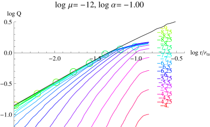
Figure 18: The cumulative distribution $Q$ as a function of $r/r_{ta}$. Same as 16 except $G\mu=10^{-12}$.

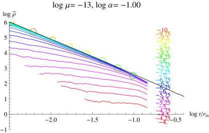
Figure 19: The number density within a radius $r/r_{ta}$ for $G\mu=10^{-13}$ and $\alpha=10^{-1}$ (same as Figure 16).

8 Current Halo Profile

The actual halo profile is more complicated than the examples constructed in the previous section because it involves loops of many sizes created over a range of epochs. Results for two specific formation scenarios are illustrated in this section.

8.1 Measures of the Loop Distribution

The cumulative distribution $N_{AB}(<r)=\int dl\int_{0}^{r}drdN_{AB}/dldr$ and the length-weighted cumulative distribution $L_{AB}(<r)=\int ldl\int_{0}^{r}drdN_{AB}/dldr$ provide summary information about the number and total length of all loops bound to the galaxy. These quantities are normalized with respect to $N_{A}$ and $L_{A}$, the equivalent quantities expected to be present in homogeneous space (eq. 51). A measure of the cumulative number of loops bound to the galaxy compared to the total within the turn-around volume is

$${\cal Q}(<r)=\frac{N_{AB}(<r)}{N_{A}(<r_{ta})}$$ (78)

If all loops behaved dynamically like cold dark matter particles then one would expect ${\cal Q}(<r)$ to resemble $Q_{AB}(<r)$ (eq. 70).

In a similar manner, start with the average number density of alive, bound loops within radius $r$

$${\bar{n}_{AB}}(r)=\frac{N_{AB}(<r)}{V(r)}$$ (79)

and the average number density of alive loops in homogeneous space ${\bar{n}_{A}}=N_{A}(<r)/V(r)$. A measure of the average overdensity of loops bound to the galaxy is

$${\bar{\cal N}}(<r)=\frac{{\bar{n}_{AB}}(<r)}{\bar{n}_{A}}$$ (80)

To the extent that loops behave like cold dark matter then one expects ${\bar{\cal N}}(<r)$ to vary like $Q_{AB}(<r)(r_{ta}/r)^{3}$.

Let $X$ be the average over the length distribution of some function; denote by $X^{(i)}$ the length-weighted moment of the function times $l^{i}$ for $i=1$, $2$,… The first moment corresponds to total length or energy.

The substitutions $N_{AB}\to N_{AB}^{(1)}=L_{AB}$ and $N_{A}\to N_{A}^{(1)}=L_{A}$ leads to cumulative and density with respect to energy instead of numbers. In an obvious fashion, let ${\cal Q}(<r)\to{\cal Q}^{(1)}(<r)=\frac{L_{AB}(<r)}{L_{A}(<r_{ta})}$, ${\bar{n}_{AB}}(r)\to{\bar{n}_{AB}^{(1)}}$, ${\bar{n}_{A}}\to{\bar{n}_{A}^{(1)}}$, and ${\bar{\cal N}}(<r)\to{\bar{\cal N}^{(1)}}(<r)$.

8.2 Point: Large Loops from Fragmentation Model

A model in which all the long string length goes into sub-horizon-scale loops will be discussed first. The model parameters are $\delta_{frag}=1$, $\alpha_{L}=10^{-3}$, $\alpha_{U}=10^{-1}$, $\mu=10^{-15}$-$10^{-9}$ with $f(x)\propto x^{-\beta}$. Let $g(x,t)$ be integrated over the birth rate density:

$$I[g] = \int dl\int dt\frac{f\left(\frac{l}{ct}\right)}{c^{4}t^{5}}a(t)^{3}g(x,t)$$ (81)

$$\propto \int dxx^{-\beta}\int dtt^{3\nu-4}g(x,t)$$ (82)

For $g=1$ the integral $I[g]$ is proportional to total number of loops born. For matter (radiation) era $\nu=2/3$ ($1/2$) the result varies like $1/t$ ($1/t^{3/2}$) and the number of loops is dominated by the earliest epochs. For $g=l=xt$, $I[g]$ is proportional to total length of loops born and the result varies like $\log t$ ($1/t^{1/2}$). For $\beta<1$ large $x$ loops dominate as measured by number and by length.

The cumulative number $\cal Q$ is shown in figure 20 for $\mu=10^{-15}$ with and without the cutoff imposed by the gravitational wave recoil. $Q_{AB}$ for cold dark matter (the black line) provides a point of reference. All three cumulative distributions are close at small radii ($r/r_{ta}<10^{-2.5}$ or approximately $<3$ kpc). The rocket is effective at depleting the old and hence small loops that would otherwise be present at large radii. Since loop numbers are dominated by formation at the earliest epochs, the characteristic signature of the recoil effect is the depletion of large numbers of loops at large radii. The inner regions are not immune to the depletion but it is less severe.

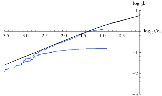
Figure 20: Clustering for $G\mu=10^{-15}$ by number of loops for $f$ constant ($\beta=0$), loop size $l=\alpha/H$, $(\alpha_{L},\alpha_{U})=(10^{-3},10^{-1})$, matter era expansion dynamics ($a\propto t^{\nu}$ with $\nu=2/3$). The black line is $\log Q_{AB}(<r)$ for cold dark matter, the blue lines are $\log{\cal Q}$ for loops with (lower) and without (upper) the gravitational wave recoil (the rocket effect).

By contrast ${\cal Q}^{(1)}$ weights loops by today’s length. This distribution samples a broader range of times. The three cumulative distributions (with and without rocket and cold dark matter) now have a very different set of relationships. There are two qualitative observations: recoil makes little apparent difference and the amplitude of the cumulative loop distribution lies below the cold dark matter one.

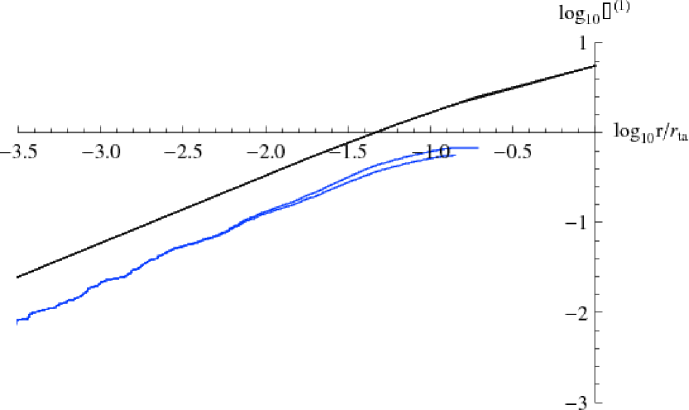
Figure 21: Clustering by energy of loops (same parameters as figure 20). The black line is $\log Q_{AB}(<r)$ for cold dark matter, the blue lines are $\log{\cal Q}^{(1)}$ for loops with (lower) and without (upper) the gravitational wave recoil (the rocket effect).

Recoil is not dramatic in ${\cal Q}^{(1)}$ because only a small contribution to total length is made by loops near the end of their lifetimes. This can be understood by revisiting figure 9 which displays the bounds on formation time and string tension. At fixed tension the logarithmic interval between the lifetime (red diagonal) line and the current epoch is proportional to total loop length created and present in homogeneous space. Only part binds to the galaxy, the interval between the lifetime line and the capture time (turquoise horizontal) line. The rocket cuts out the space below the acceleration condition (green diagonal). For small $G\mu$ many decades lie above the acceleration line and below the capture time so it is difficult to see the effect of the rocket on the length-weighted loop distribution.

Insensitivity of ${\cal Q}^{(1)}$ is not a prerequisite for clustering but an interesting consequence of the weighting and scale factor. One expects the rocket to have a more visible influence on ${\cal Q}^{(1)}$ in the radiation era when the distribution is $\propto t^{-1/2}$ not $\log t$.

The second observation, that the amplitude of the cumulative distribution lies below the cold dark matter comparison, is related to the necessity of slowing down enough for capture. Again, referring to figure 9, at fixed $G\mu$ loops born between the capture line and the current epoch are present in homogeneous space but cannot bind to the galaxy today. The effect lowers the amplitude relative to the cold dark matter scenario where there is no such constraint. At first glance, the figure would suggest that the amplitude be diminished by $\sim 2$ (i.e. at $G\mu=10^{-15}$ about half the decades lie above the capture line and half below). The figure illustrates $v_{i}=0.1$ whereas the simulation velocities are larger (rms dispersions are $0.5-0.9$). The excluded region in the figure increases and accounts for the factor of $3-4$ diminution in amplitude observed in the simulation.

As the tension increases the natural expectation is that the curves should fall away from the cold dark matter analog since $H\tau$ diminishes and less damping will be possible. In figure 9 this corresponds to trying to move to the right and the available phase space shrinks. The cumulative number $\cal Q$ are shown in figure 22 for range of string tensions $10^{-15}$-$10^{-10}$. The lowermost profiles have tensions $G\mu=10^{-10}$ and $10^{-11}$ and fulfill this expectation. However, a striking feature is that all curves with $G\mu\mathbin{\lower 3.0pt\hbox{$\hbox to0.0pt{\raise 5.0pt\hbox{$\char 60\relax$}\hss}\mathchar 29208\relax$}}10^{-12}$ are bunched together. They track the cold dark matter profile at small radii and are stripped beyond a characteristic radius. Without the rocket effect the same subset of curves closely tracks the cold dark matter profile to about $r/r_{ta}\sim 0.1$ (at which point deciding whether or not a loop is bound is problematic).

Since most loops are created at early times, in the absence of dynamics most have ages $\sim t_{0}$. The gravitational wave acceleration of such loops is $a_{R}\sim\Gamma_{P}c/\Gamma_{E}t_{0}$. Setting this equal to $\chi_{crit}|\nabla\phi|$ gives the characteristic radial scale $\chi_{crit}v_{c}^{2}\Gamma_{E}t_{0}/(c\Gamma_{P})\sim 2.3$ kpc or $\log r/r_{ta}\sim-2.7$, approximately what is observed in the simulations and independent of $G\mu/c^{2}$.

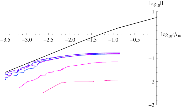
Figure 22: String tensions $G\mu=10^{-10}$ to $10^{-15}$ in powers of ten, bottom to top with all other parameters the same as figure 20). The black line is $\log Q_{AB}(<r)$ for cold dark matter, the colored lines are $\log{\cal Q}$ (all with rocket effect). For $r/r_{ta}<10^{-2.5}$ the group with $G\mu<10^{-12}$ are numerically indistinguishable given the finite Monte-Carlo sample.

Profiles with loops weighted by length are shown in 23. Because the loop distribution is logarithmic, the measures are not dominated by the loops formed at the earliest times nor is the rocket effect a dominant influence on the shape. As tension decreases, the cumulative approaches the cold dark matter limit albeit slowly.

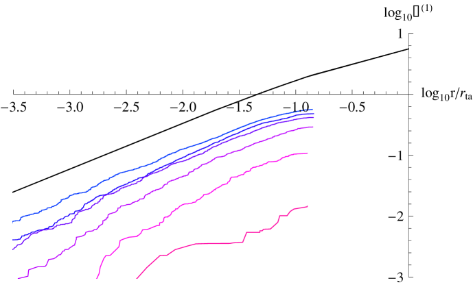
Figure 23: Clustering by energy of loops with string tensions $G\mu=10^{-10}$ to $10^{-15}$ in powers of ten, bottom to top (colored lines) and all other parameters the same as figure 20). The black line is $\log Q_{AB}(<r)$ for cold dark matter, the colored lines are $\log{\cal Q}^{(1)}$ for loops (all with rocket effect).

The average interior density within a radius is displayed in figures 24 (number) and 25 (length). They illustrate that the loop clustering follows that of the dark matter.

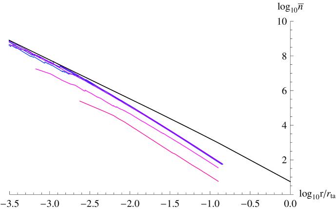
Figure 24: Mean interior number density of loops $\log_{10}{\bar{\cal N}}(<r)$ (relative to unclustered loop population, including rocket effect). String tensions $G\mu=10^{-10}$ to $10^{-15}$ in powers of ten, bottom to top (colored lines) and all other parameters the same as figure 20). The black line is $\log Q_{AB}(<r)(r_{ta}/r)^{3}$ for cold dark matter. The infall model has turn-around radius $r_{ta}=1.1$ Mpc.

Figure 26 shows that varying $\beta$, the slope of the loop distribution function, has little effect. The significance of this observation is not that the change in $\beta$ is ignorable but that it is subsumed by scaling with respect to the homogeneous results.

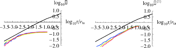
Figure 26: Cumulative distributions for $\beta$=$0$ (blue), $1$ (green) and $1.63$ (red) for for $G\mu=10^{-15}$ for number (left) and energy (right) of loops. The remaining parameters are the same as figure 20.

All the calculations in this section will be altered by treating the loop production during the radiation era with the correct scale factor $a(t)\propto t^{1/2}$. The weighting of the birth rate in the comoving volume will shift from a logarithmic distribution to one that $\propto t^{-1/2}$. New results will be calculated in the future but one can infer that this new ${\cal Q}^{(1)}$ will have properties intermediate between ${\cal Q}$ (dominated by early time production) and ${\cal Q}^{(1)}$ (logarithmic) calculated thus far.

8.3 Counterpoint: Small Loops by Cusp Formation

According to current estimates 80-90% of the horizon-crossing string ends up forming small loops. They are unlikely to cluster well because they are born moving fast and they have intrinsically small lengths. However, they have a broad range in $x=l/t$ and the relativistic kinematic effects are non-trivial (time dilation, energy shifts). So it is of interest to investigate the degree of clustering within the galaxy. For a simplified, canonical treatment assume 100% efficiency ($\delta=1$) for chopping long strings into loops characterized by $f(x)\propto x^{-\beta}$ over the range $x=(x_{GW},1)$. Here, the power law index $\beta=3-2\chi$ and $\chi=0.25$ in the matter era. The loops are weighted in number and mass to the low cutoff at the gravitational wave damping scale $x_{GW}=20.\left(G\mu\right)^{1+2\chi}$. The velocity dispersion of newly formed loops is given by the ultra-relativistic theoretical result eq. 58.

Results for $G\mu=10^{-15}$ are presented in figure 27 for the cumulative number distribution ${\cal Q}$ and the cold dark matter behavior $Q_{AB}$. It is apparent that only a very small fraction of the loops generated by cusp formation are able to live long enough to slow down and bind to the galaxy. Recall that homogeneous space has ${\cal Q}=1$; the majority of small living loops in proximity with the galaxy are not bound to it. The figure also illustrates the effect of turning off the rocket effect and starting from a less-relativistic velocity distribution function. These change ${\cal Q}$ in the manner expected but still leaves the relative numbers small. A similar picture emerges from the cumulative length distribution ${\cal Q}^{(1)}$ in figure 28.

Figure 27: The yellow unadorned line is the cumulative number distribution of loops ($\log{\cal Q}$) for $G\mu=10^{-15}$ in cusp-generated loop formation during the matter era ($\nu=2/3$, $\chi=0.25$, ${\bar{v_{\infty}^{2}}}=0.35$, $1/\gamma_{s}^{2}=10$, $(x_{L},x_{H})=\left(x_{GW},1\right)$ with $x_{GW}=20.\mu^{1+2\chi}$ and with theoretically determined ultra-relativistic velocity distribution eq. 58). The black line is $\log Q_{AB}(<r)$ for cold dark matter. The lines with dots represent altering the standard model assumptions: suppress rocket effect (blue), adopt less relativistic initial velocity distribution (red), and combined (green).

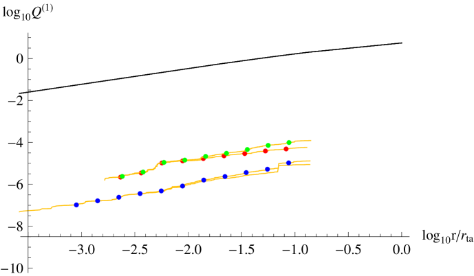
Figure 28: Cumulative energy distribution of loops ($\log{\cal Q}^{(1)}$); identical parameters as figure 27.

The average interior number and energy densities are shown in figures 29 and 30. The canonical model reaches the background number (energy) density at $r/r_{ta}=10^{-2.9}$ ($10^{-2}$). The smallest $r/r_{ta}$ at which the infall model will be a reasonably accurate physical description of the galaxy is $\sim 10^{-3}$.

Figure 29: Average interior number density of loops ($\log{\bar{\cal N}}$); identical parameters as figure 27.

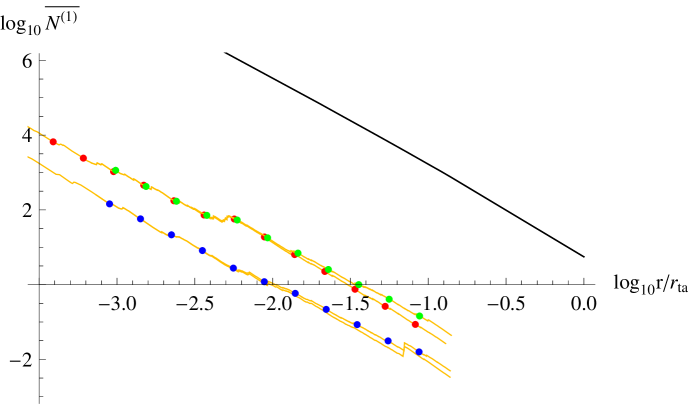
Figure 30: Average interior energy density of loops ($\log{\bar{\cal N}^{(1)}}$); identical parameters as figure 27.

A comparison of ${\cal Q}^{(1)}$ for tensions $G\mu=10^{-15}$-$10^{-12}$ shows that increasing $\mu$ increases the ${\cal Q}^{(1)}$. Essentially, the gravitational wave cutoff $x_{GW}\propto\mu^{1.5}$ increases and each horizon crossing string makes more large loops which live longer and move more slowly. The range of uncertainty is shown by comparing the results for velocities drawn from the less relativistic Ref. [115].

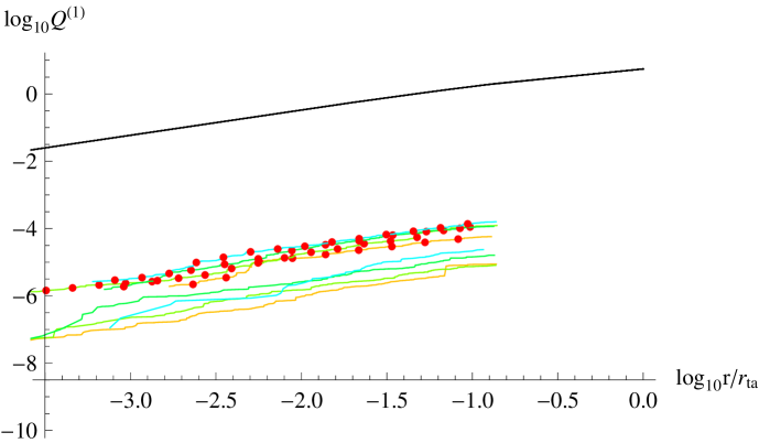
Figure 31: The cumulative energy distribution of loops ($\log{\cal Q}^{(1)}$) for $G\mu=10^{-12}-10^{-15}$ (yellow to blue) in cusp-generated loop formation during the matter era ($\nu=2/3$, $\chi=0.25$, ${\bar{v_{\infty}^{2}}}=0.35$, $1/\gamma_{s}^{2}=10$, $(x_{L},x_{H})=\left(x_{GW},1\right)$ with $x_{GW}=20.\ \mu^{1+2\chi}$ and with theoretically determined ultra-relativistic velocity distribution eq. 58). The black line is $\log Q_{AB}(<r)$ for cold dark matter. The lines with red dots show the effect of altering the standard model assumptions to adopt less relativistic initial velocity distribution. All lines include rocket effect.

9 Conclusions

Cosmic superstrings are produced towards the end of brane inflation, a scenario in modern superstring theory. As string tension $\mu$ decreases and/or formation size $\alpha$ increases (where $\alpha$ is roughly the fraction of the horizon), then the timescale for the loop to evaporate by gravitational emission $\tau\propto\alpha/\mu$ increases. This has important consequences for the abundance of strings as potentially observable astrophysical objects[67, 5]. Although born moving at close to the speed of light, long-lived loops damp by the expansion of the universe and fall into potential wells created by cold dark matter and baryons after equipartition[5, 6].

This paper explores the dynamics of loops in the vicinity of the galaxy. The model used to represent the growing galaxy is a self-similar, radial infall model for the cold dark matter component. The form for the perturbed FRW metric then provides the playground for the fully relativistic treatment of string loop dynamics.

A succession of increasingly complex dynamical investigations addresses the basic question “how did the halo get its loops?” These include: capture of fast moving objects by the growing perturbation, recoil by radiated gravitational waves, protection of tightly bound orbits by adiabatic invariance and a critical transition from confined to free, liberated motion.

The basic picture that emerges is straightforward. Loops damp by cosmological expansion coming nearly to rest and some find themselves in the vicinity of a growing matter perturbation. These fall into the perturbation and, like cold dark matter, acquire radial orbits with scale comparable to the turn-around radius. They linger at roughly fixed physical radius while both the galaxy and the turn-around radius grow with age. A snapshot of the galaxy would reveal the oldest loops near the center and the newest ones on the periphery. The oldest loops are also the smallest loops because the horizon size $\propto t$.

All loops shrink by emission of gravitational wave energy and are subject to significant recoil because the antenna pattern is highly anisotropic. The length decreases and the non-gravitational acceleration increases in tandem. The specific assumptions about recoil made in this paper are conservative in the sense that they maximize the importance of the rocket effect and minimize the possibility of loop clustering.

For loops of a given size and age the galaxy is stripped from the outside in. Conversely, these loops are retained latest in the central parts of the potential well where the binding is greatest. Eventually as the length vanishes and the acceleration diverges all will be removed.

The halo is grown from loops of different sizes accreted over a range of times subject to the dynamical capture process. Since small loops move faster than large ones at birth two different sized loops born at the same time will generally not accrete at the same time. The halo is a mix of loops with a range of sizes and ages at a given apocenter.

Two broad classes for loop formation were characterized. Loops directly generated by fragmentation (“large” loops) and those mediated by cusp formation (“small” loops). It was anticipated and verified that only the large loops cluster about the galaxy to a significant extent.

The bottom line results for large loops are presented in figures 24 (density of the number of loops within the galaxy relative to the unclustered, homogeneous value) and 25 (density of length or energy of loops). There is a substantial degree of enhancement in both number and energy density at a broad range of galactocentric radii that depends upon string tension.

The bottom line results for small loops are presented in figures 29 (number density) and 30 (energy density). Little enhancement is observed and that only at radii $\mathbin{\lower 3.0pt\hbox{$\hbox to0.0pt{\raise 5.0pt\hbox{$\char 60\relax$}\hss}\mathchar 29208\relax$}}1$ kpc where the radial infall model is not applicable.

Some essential input physics needs improvement:

• The loop production function needs to be characterized accurately, especially the fraction of horizon-crossing strings that form large loops ($\delta_{frag}$) and the characteristic scale of the large loops ($x_{U}$).

• The secular changes to the loop parameters as the loop shrinks need to be calculated. This determines the timescale for intrinsic variation of the recoil direction, the possibility of loop precession (angular momentum changes not along the angular momentum direction), and the propensity to convert non-self-intersecting to self-intersecting loops.

These have direct implications for the number and size of the loops that are formed, the efficacy of the rocket effect and the loop lifetime.

From the viewpoint of clustering dynamics these areas need attention:

• The string network and background cosmology need to be calculated in the context of $\Lambda$CDM cosmology. All calculations here use the Einstein-de Sitter non-relativistic matter model.

• The galaxy formation model should be made more realistic and consistent with structure formation in $\Lambda$CDM cosmology.

• Dissipative effects may be important in two contexts: dynamical friction can slow down loops before clustering begins and can remove energy from loops orbiting within the galaxy.

• Loop-loop interactions may develop at the galactic center as nearly radial orbits converge. If such interactions do occur then the small loops formed by intercommutation may acquire relativistic velocities and be ejected.

The first two items should generally improve the treatment of the loop distribution and bring it up to date vis-a-vis modern cosmology. The third and fourth items are unique to the loop dynamics. They may increase and decrease, respectively, the theoretically calculated halo densities. A paper on extending the current results to loops born in the radiation era is being prepared.

From the perspective of detectable astrophysical signatures a clustered loop halo is a natural source of signals for the following experiments: direct detection of gravitational wave emission, pulsar timing variation, and microlensing. Experiments sensitive to the local population, especially microlensing of Galactic stars, will see the most significant impact of clustering.

Appendix A Equations of Motion in Inhomogeneous FRW

The 4-velocity and direction of the 4-impulse are parameterized in terms of $v$, ${\hat{v}}$, $n$, ${\hat{n}}$ according to

$$V^{\mu} = \left(\frac{\sqrt{1+v^{2}}}{\alpha_{\psi}},\frac{v{\hat{v}}^{i}}{a\alpha_{\Phi}}\right)$$ (83)

$$N^{\mu} = \left(\pm\frac{\sqrt{n^{2}-1}}{\alpha_{\psi}},\frac{n{\hat{n}}^{i}}{a\alpha_{\Phi}}\right)$$ (84)

$$\alpha_{\Phi} = \sqrt{1+2\Phi}$$ (85)

$$\alpha_{\psi} = \sqrt{1+2\psi}$$ (86)

where $c=1$ and hat quantities are unit vectors. The sign of $N^{0}$ is the sign of ${\hat{n}}\cdot{\hat{v}}$. The equations of motion are

$$\frac{\text{dv}}{\text{dt}} = \frac{\left(\hat{n}\cdot\hat{v}\right)a_{r}n\alpha_{\psi}}{\sqrt{1+v^{2}}}-\frac{\left(\hat{v}\text{$\cdot\nabla\psi$)}\right.\sqrt{1+v^{2}}}{a\alpha_{\Phi}\alpha_{\psi}}-\frac{v\dot{a}}{a}-\frac{v\dot{\Phi}}{\alpha_{\Phi}^{2}}$$ (87)

$$\frac{d\hat{v^{i}}}{\text{dt}} = \frac{a_{r}n\alpha_{\psi}(\hat{n^{i}}-\left(\hat{n}\cdot\hat{v}\right)\hat{v^{i}})}{v\sqrt{1+v^{2}}}-\frac{\alpha_{\psi}v(\left(\hat{v}\text{$\cdot\nabla\Phi$)}\right.\hat{v^{i}}-\Phi_{,i})}{a\alpha_{\Phi}^{3}\sqrt{1+v^{2}}}+$$

$$\frac{\sqrt{1+v^{2}}(\left(\hat{v}\text{$\cdot\nabla\psi$)}\right.\hat{v^{i}}-\psi_{,i})}{a\alpha_{\Phi}\alpha_{\psi}v}$$

$$\frac{\text{dn}}{\text{dt}} = -\frac{\left(\hat{n}\text{$\cdot\nabla\psi$)}\right.\left(\hat{n}\cdot\hat{v}\right)nv}{a\alpha_{\Phi}\alpha_{\psi}\sqrt{1+v^{2}}}+\frac{\left(\hat{n}\cdot\hat{v}\right)a_{r}\alpha_{\psi}v}{\sqrt{1+v^{2}}}-\frac{\left(\hat{n}\cdot\hat{v}\right)^{2}nv^{2}\dot{a}}{a\left(1+v^{2}\right)}-\frac{\left(\hat{n}\cdot\hat{v}\right)^{2}nv^{2}\dot{\Phi}}{\alpha_{\Phi}^{2}\left(1+v^{2}\right)}$$ (89)

$$\frac{d\hat{n^{i}}}{\text{dt}} = -\frac{a_{r}\alpha_{\psi}v(\left(\hat{n}\cdot\hat{v}\right)\hat{n^{i}}-\hat{v^{i}})}{n\sqrt{1+v^{2}}}+\frac{\left(\hat{n}\cdot\hat{v}\right)v^{2}(\left(\hat{n}\cdot\hat{v}\right)\hat{n^{i}}-\hat{v^{i}})\dot{a}}{a\left(1+v^{2}\right)}+$$

$$\frac{v\left(\left(\hat{n}\text{$\cdot\nabla\psi$)}\right.\left(\hat{n}\cdot\hat{v}\right)\hat{n^{i}}\alpha_{\Phi}^{2}-\left(\hat{n}\text{$\cdot\nabla\Phi$)}\right.\alpha_{\psi}^{2}\hat{v^{i}}+\left(\hat{n}\cdot\hat{v}\right)\alpha_{\psi}^{2}\Phi_{,i}-\left(\hat{n}\cdot\hat{v}\right)\alpha_{\Phi}^{2}\psi_{,i}\right)}{a\alpha_{\Phi}^{3}\alpha_{\psi}\sqrt{1+v^{2}}}+$$

$$\frac{\left(\hat{n}\cdot\hat{v}\right)v^{2}(\left(\hat{n}\cdot\hat{v}\right)\hat{n^{i}}-\hat{v^{i}})\dot{\Phi}}{\alpha_{\Phi}^{2}\left(1+v^{2}\right)}$$

$$\frac{\text{dx}^{i}}{\text{dt}} = \frac{\alpha_{\psi}v\hat{v^{i}}}{a\alpha_{\Phi}\sqrt{1+v^{2}}}$$ (91)

$$\frac{\text{da}_{r}}{\text{dt}} = \frac{\Gamma_{E}a_{r}{}^{2}\alpha_{\psi}}{\Gamma_{P}\sqrt{1+v^{2}}}$$ (92)

Terms have been organized into 3-vector dot products ($(d\cdot e)\equiv\sum_{i=1,3}d^{i}e^{i}$), the explicit index $i$ runs $1-3$ and time derivatives are indicated ${\dot{e}}\equiv\frac{de}{dt}$.

Appendix B Relating Center of Mass and FRW Accelerations

Let $V^{\mu}$ be the initial 4-velocity of the string center of mass in the FRW frame. For clarity, let $V_{(x)}^{\alpha}$ be the components in the FRW frame (“x”) and first define a transformation to an orthonormal frame (“y”) by

$$dy^{0} = \sqrt{1+2\psi}dx^{0}$$ (93)

$$dy^{i} = a\sqrt{1+2\Phi}dx^{i}$$ (94)

$$V_{(y)}^{\alpha} = \frac{\partial y^{\alpha}}{\partial x^{\beta}}V_{(x)}^{\beta}$$ (95)

Second, introduce a Lorentz boost to the rest frame (“z”; designated $\Lambda^{\alpha}_{\beta}$) i.e. $\Lambda V_{(y)}\to V_{(z)}=(1,0,0,0)$. Explicitly,

$$\Lambda^{\alpha}_{\beta} = \frac{\partial z^{\alpha}}{\partial y^{\beta}}$$ (96)

$$= \left(\begin{array}[]{cc}V_{(y)}^{0}&-V_{(y)}^{i}\\ -V_{(y)}^{i}&1+\frac{(V_{(y)}^{0}-1)V_{(y)}^{i}V_{(y)}^{j}}{\sum_{k}(V_{(y)}^{k})^{2}}\end{array}\right)$$ (99)

The impulse in the string center of mass frame is $a_{(z)}^{\alpha}=(0,a_{(z)}^{i})=a_{r}(0,n_{(z)}^{i})$ where $n_{(z)}^{i}$ is a unit-vector. The 4-impulse in the FRW frame is

$$a_{(x)}^{\alpha} = \frac{\partial x^{\alpha}}{\partial y^{\beta}}\frac{\partial y^{\beta}}{\partial z^{\gamma}}a_{(z)}^{\gamma}$$ (100)

$$= a_{r}\left(\begin{array}[]{c}a\sqrt{\frac{1+2\Phi}{1+2\psi}}V_{(x)}\cdot n_{(z)}\\ \frac{1}{a\sqrt{1+2\Phi}}\left(n_{(z)}^{i}+\left(V_{(x)}^{0}\sqrt{1+2\psi}-1\right)V_{(x)}^{i}\frac{V_{(x)}\cdot n_{(z)}}{V_{(x)}\cdot V_{(x)}}\right)\end{array}\right)$$ (103)

$$= a_{r}N^{\alpha}.$$ (104)

where $V_{(x)}\cdot n_{(z)}=\sum_{k=1,3}V_{(x)}^{k}n_{(z)}^{k}$ and $V_{(x)}\cdot V_{(x)}=\sum_{k=1,3}V_{(x)}^{k}V_{(x)}^{k}$. This specifies the initial $N^{\alpha}$.

It remains to determine the scalar $a_{r}$. In the center of mass of the loop the rates of energy and momentum loss are

$$\frac{dl_{(z)}}{dz^{0}} = -\Gamma_{E}\left(G\mu\right)$$ (105)

$$a_{r} = \Gamma_{P}\left(G\mu\right)\frac{1}{l_{(z)}}$$ (106)

Since, $dz^{0}=\frac{dx^{0}}{V^{0}_{(x)}}$ the length may be straightforwardly expressed in terms of the FRW time

$$l_{(z)}=l_{(z),init}-\Gamma_{E}\left(G\mu\right)\int_{x^{0}_{init}}\frac{dx^{0}}{V^{0}_{(x)}}$$ (107)

Loops at highly relativistic speeds in the FRW frame have extended lifetimes because their center of mass clocks advance more slowly. It is convenient to express the evolution of $a_{r}$ directly in the FRW frame using the global time coordinate

$$\frac{d}{dx^{0}}\left(\frac{1}{a_{r}}\right)=-\frac{\Gamma_{E}}{\Gamma_{P}V_{x}^{0}}$$ (108)

After $a_{r}N^{\alpha}$ is initially set the entire calculation can be carried out in the FRW frame.

Appendix C Variants of Figure 9

Figure 32 shows the bounds on the formation time and string tension for a loop with initial velocity $v_{i}=0.1$ captured and retained at physical radius 30 kpc. It is essentially the same as 9 but the black lines are based on $v$ found by numerical calculations using eqs. (32)-(35) for aligned and anti-aligned rockets rather than by the analytic expressions in §5.2. It generally validates the analytic approximations, however, it shows the existence of some additional phase space for capture when the relative directions of impulse and initial velocity vary. The green line is the retention criterion based on the critical acceleration at the current epoch.

Figure 33 is similar to the one above but applies to capture at a smaller physical radius 10 kpc. The formation time must be earlier and the acceleration limit approaches the loop lifetime limit.

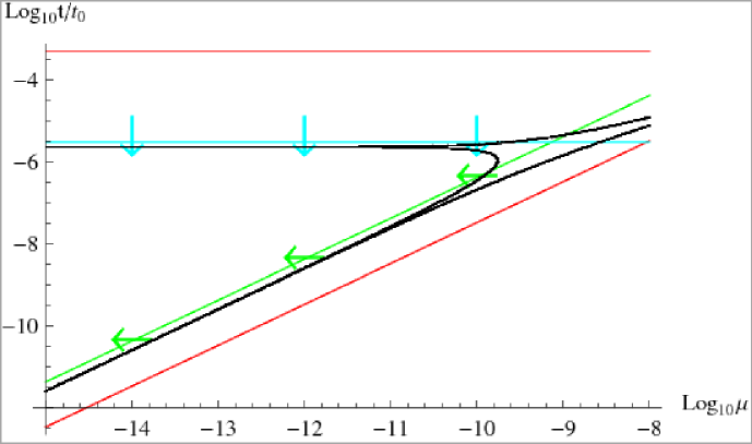
Figure 32: Same as 9 except that $v$ is calculated with the full relativistic equations of motion for aligned and anti-aligned rockets to determine capture and the numerical experiments for randomly oriented rockets are omitted.

Figure 33: Same as 32 except for physical radius 10 kpc. The red lines (damping to the characteristic rotation velocity and lifetime) are unchanged. All the other lines move. Capture requires earlier formation and retention allows larger $G\mu$.

Appendix D Monte-Carlo Dynamics

The probability that the particle is bound with position $\vec{x}$, momentum $\vec{v}$ and length $l$ today

$$\frac{dP_{bnd}}{d{\vec{x}}d{\vec{v}}dl}=\frac{1}{\tilde{V}}\int d{\vec{x}^{\prime}}d{\vec{v}^{\prime}}d{l^{\prime}}\frac{dP}{d\vec{v}^{\prime}}\frac{dP}{dl^{\prime}}\delta^{3}({\vec{x}}-{\vec{X}})\delta^{3}({\vec{v}}-{\vec{V}})\delta(l-L)\theta_{AB}\left({\vec{x}},{\vec{v}}\right)$$ (109)

where $\vec{X}$, $\vec{V}$ and $L$ are the formal time-dependent solutions for initial position $\vec{x}^{\prime}$, momentum $\vec{v}^{\prime}$ and length $l^{\prime}$ at time $t^{\prime}$. The integration is over the distribution of position and momentum while $l^{\prime}=l_{i}$ and $t^{\prime}=t_{i}$ are fixed.

There are some significant computational simplifications. First, only the properties of the bound particles with $l>0$ are of interest. To avoid sampling initial conditions which imply $\theta_{B}=0$ and/or loops that have evaporated use the following approximations. In flat FRW space, directly integrate the motion and length of a particle with given initial momentum from $t_{i}$ to $t_{0}$. The particle must live to the current epoch and be able to enter the spherical volume defined by today’s turn-around radius or there is no chance of it being accreted. This limits the minimum length $l^{\prime}$ as well as the maximum distance and the range of angles between $\hat{x}$ and $\hat{v}$ that need to be sampled. For acceptable $l^{\prime}$ the Monte-Carlo points are weighted by the ratio of the volume actually sampled to the total volume.

For efficiency order the kinematic integrals (1) magnitude of $v^{\prime}$, (2) magnitude of $x^{\prime}$, (3) direction $\hat{x}^{\prime}$ and (4) direction $\hat{p}^{\prime}$. First, sample $v^{\prime}$ according to $dP/dv^{\prime}$ (weight is 1). Second, calculate $x_{max}$, the maximum initial displacement from the perturbation center that a particle can have and still reach the turn-around volume by today, and sample $x^{\prime}$ from the volume associated with $x_{max}$ (weight is $4\pi x_{max}^{3}/3\tilde{V}$). Third, sample $\hat{x}^{\prime}$ in the full sphere (weight is 1). Fourth, sample $\hat{v}^{\prime}$ from the maximum angular range that allows motion from $x^{\prime}$ to reach the turn-around volume by today (weight is ratio of the angular extent sampled to the full $4\pi$ extent).

To generate the final distribution, weight each bound particle according to the sampling above. In the end, ignore the orbital phase of the particle, i.e. marginalize the two-dimensional distribution to give the distribution of semi-major axes

$$\frac{dP_{bnd}}{drdl}=\int d{\vec{x}}d{\vec{v}}\frac{dP_{bnd}}{d{\vec{x}}d{\vec{v}}d{l}}\delta(r-R)$$ (110)

where $R=R({\vec{x}},{\vec{v}},t_{0})$ is the formal expression for the semi-major axis in terms of the current phase space coordinates.

The second simplification is to recognize that once a particle is bound to the perturbation the physical dimensions of its orbit are fixed if the rocket effect is ignored. Therefore, its unnecessary to integrate all particles from $t_{i}$ to $t_{0}$. Stop once a particle has passed back and forth through the perturbation center several times and been captured. The error (i.e. the characteristic size of the change in $r$ in the future due to the growth of the perturbation) can be inferred by the variation in the relative heights of the peaks in figure 3. To the extent that the orbit is exactly radial, one could extrapolate from the last calculated $r$ to the asymptotic one. In this work, the integration after $N_{c}$ bounces ($N_{c}=3$-$8$) is halted and the value of $r$ at that time is adopted. A check that the final results are insensitive to $N_{c}$ is made.

The third simplification (used in §7 and 8) is to ignore the rocket effect before capture and apply the retention and lifetime criteria at the current epoch. Retention is more stringent than capture so little error is made. This allows the same simulation to be used for different choices of $\mu$.

A fourth simplification is to work directly with the cumulative distribution rather than the differential one. It is ultimately necessary to record only the weight and the semi-major axis of the bound particles generated by Monte-Carlo sampling. A sort of the semi-major axis of the final sample allows simple construction of the cumulative probability distribution from the weights.

References

- [1] T. W. B. Kibble, Topology of cosmic domains and strings., Journal of Physics A Mathematical General 9 (1976) 1387–1398.
- [2] I. B. Zeldovich, Cosmological fluctuations produced near a singularity, Monthly Notices of the Royal Astronomical Society 192 (Sept., 1980) 663–667.
- [3] A. Vilenkin, Cosmological density fluctuations produced by vacuum strings, Physical Review Letters 46 (Apr., 1981) 1169–1172.
- [4] A. Vilenkin, Cosmic strings, Physical Review D 24 (Oct., 1981) 2082–2089.
- [5] D. F. Chernoff and S. H. H. Tye, Cosmic string detection via microlensing of stars, 0709.1139 (Sept., 2007).
- [6] M. R. DePies and C. J. Hogan, “Harmonic gravitational wave spectra of cosmic string loops in the galaxy.” http://adsabs.harvard.edu/abs/2009arXiv0904.1052D, Apr., 2009.
- [7] A. Albrecht and P. J. Steinhardt, Cosmology for grand unified theories with radiatively induced symmetry breaking, Physical Review Letters 48 (Apr., 1982) 1220–1223.
- [8] A. H. Guth, Inflationary universe: A possible solution to the horizon and flatness problems, Physical Review D 23 (1981) 347–356.
- [9] A. D. Linde, A new inflationary universe scenario: a possible solution of the horizon, flatness, homogeneity, isotropy and primordial monopole problems., Physics Letters B 108 (1982) 389–393.
- [10] S. Buchan, B. Shlaer, H. Stoica, and S. H. Tye, Inter-brane interactions in compact spaces and brane inflation, Journal of Cosmology and Astro-Particle Physics 02 (Feb., 2004) 013.
- [11] C. P. Burgess, M. Majumdar, D. Nolte, F. Quevedo, G. Rajesh, and R. Zhang, The inflationary brane-antibrane universe, Journal of High Energy Physics 07 (July, 2001) 047.
- [12] G. Dvali and S. H. Tye, Brane inflation., Physics Letters B 450 (Mar., 1999) 72–82.
- [13] G. Dvali, Q. Shafi, and S. Solganik, “D-brane inflation.” http://adsabs.harvard.edu/abs/2001hep.th….5203D, May, 2001.
- [14] S. B. Giddings, S. Kachru, and J. Polchinski, Hierarchies from fluxes in string compactifications, Physical Review D 66 (Nov., 2002) 106006.
- [15] P. Horava, “Type IIA D-Branes, K-Theory, and matrix theory.” http://adsabs.harvard.edu/abs/1998hep.th…12135H, Dec., 1998.
- [16] S. Kachru, R. Kallosh, A. Linde, and S. P. Trivedi, de sitter vacua in string theory, Physical Review D 68 (Aug., 2003) 46005.
- [17] S. Kachru, R. Kallosh, A. Linde, J. Maldacena, L. McAllister, and S. P. Trivedi, Towards inflation in string theory, Journal of Cosmology and Astro-Particle Physics 10 (Oct., 2003) 013.
- [18] A. Sen, Stable non-BPS bound states of BPS d-branes, Journal of High Energy Physics 08 (Aug., 1998) 010.
- [19] A. Sen, SO(32) spinors of type i and other solitons on brane-antibrane pair, Journal of High Energy Physics 09 (Sept., 1998) 023.
- [20] S. H. Tye, Brane inflation: String theory viewed from the cosmos, vol. 737, p. 949, 2008.
- [21] E. Witten, D-branes and k-theory, Journal of High Energy Physics 12 (Dec., 1998) 019.
- [22] E. J. Copeland, R. C. Myers, and J. Polchinski, Cosmic f- and d-strings, Journal of High Energy Physics 06 (June, 2004) 013.
- [23] G. Dvali and A. Vilenkin, Formation and evolution of cosmic d strings, Journal of Cosmology and Astro-Particle Physics 03 (Mar., 2004) 010.
- [24] H. Firouzjahi and S. H. Tye, Brane inflation and cosmic string tension in superstring theory, Journal of Cosmology and Astro-Particle Physics 03 (Mar., 2005) 009.
- [25] M. G. Jackson, N. T. Jones, and J. Polchinski, Collisions of cosmic f- and d-strings, Journal of High Energy Physics 10 (Oct., 2005) 013.
- [26] N. Jones, H. Stoica, and S. H. Tye, Brane interaction as the origin of inflation, Journal of High Energy Physics 07 (July, 2002) 051.
- [27] N. T. Jones, H. Stoica, and S. H. Tye, The production, spectrum and evolution of cosmic strings in brane inflation, Physics Letters B 563 (June, 2003) 6–14.
- [28] S. Sarangi and S. H. Tye, Cosmic string production towards the end of brane inflation, Physics Letters B 536 (June, 2002) 185–192.
- [29] A. Sen, Rolling tachyon, Journal of High Energy Physics 04 (Apr., 2002) 048.
- [30] A. Sen, Tachyon matter, Journal of High Energy Physics 07 (July, 2002) 065.
- [31] S. E. Shandera and S. H. Tye, Observing brane inflation, Journal of Cosmology and Astro-Particle Physics 05 (May, 2006) 007.
- [32] A. Albrecht and N. Turok, Evolution of cosmic strings, Physical Review Letters 54 (Apr., 1985) 1868–1871.
- [33] B. Allen and E. P. S. Shellard, Cosmic-string evolution - a numerical simulation, Physical Review Letters 64 (1990) 119–122.
- [34] A. Avgoustidis and E. P. Shellard, Effect of reconnection probability on cosmic (super)string network density, Physical Review D 73 (Feb., 2006) 41301.
- [35] D. P. Bennett and F. R. Bouchet, Evidence for a scaling solution in cosmic-string evolution, Physical Review Letters 60 (1988) 257–260.
- [36] F. Dubath, J. Polchinski, and J. V. Rocha, Cosmic string loops, large and small, Physical Review D 77 (June, 2008) 123528.
- [37] C. J. Martins and E. P. Shellard, Fractal properties and small-scale structure of cosmic string networks, Physical Review D 73 (Feb., 2006) 43515.
- [38] J. Polchinski and J. V. Rocha, Analytic study of small scale structure on cosmic strings, Physical Review D 74 (Oct., 2006) 83504.
- [39] J. Polchinski and J. V. Rocha, Cosmic string structure at the gravitational radiation scale, Physical Review D 75 (June, 2007) 123503.
- [40] C. Ringeval, M. Sakellariadou, and F. R. Bouchet, Cosmological evolution of cosmic string loops, Journal of Cosmology and Astro-Particle Physics 02 (Feb., 2007) 023.
- [41] M. Sakellariadou, A note on the evolution of cosmic string/superstring networks, Journal of Cosmology and Astro-Particle Physics 04 (Apr., 2005) 003.
- [42] S. H. Tye, I. Wasserman, and M. Wyman, Scaling of multitension cosmic superstring networks, Physical Review D 71 (May, 2005) 103508.
- [43] V. Vanchurin, Cosmic string loops: large and small, but not tiny, 0712.2236 (Dec., 2007). Phys.Rev.D77:063532,2008.
- [44] V. Vanchurin, K. D. Olum, and A. Vilenkin, Scaling of cosmic string loops, Physical Review D 74 (Sept., 2006) 63527.
- [45] A. Vilenkin and E. P. S. Shellard, Cosmic Strings and Other Topological Defects. July, 2000.
- [46] A. Vilenkin, Gravitational field of vacuum domain walls, Physics Letters B 133 (Dec., 1983) 177–179.
- [47] C. Hogan and R. Narayan, Gravitational lensing by cosmic strings, Monthly Notices of the Royal Astronomical Society 211 (Dec., 1984) 575–591.
- [48] A. Vilenkin, Cosmic strings as gravitational lenses, Astrophysical Journal 282 (July, 1984) L51–L53.
- [49] A. A. de Laix, Observing long cosmic strings through gravitational lensing, Physical Review D 56 (Nov., 1997) 6193–6204.
- [50] F. Bernardeau and J. Uzan, Cosmic string lens phenomenology: Model of poisson energy distribution, Physical Review D 63 (2001) 23005.
- [51] M. Sazhin, G. Longo, M. Capaccioli, J. M. Alcal , R. Silvotti, G. Covone, O. Khovanskaya, M. Pavlov, M. Pannella, M. Radovich, and V. Testa, CSL-1: chance projection effect or serendipitous discovery of a gravitational lens induced by a cosmic string?, Monthly Notices of the Royal Astronomical Society 343 (Aug., 2003) 353–359.
- [52] M. V. Sazhin, M. Capaccioli, G. Longo, M. Paolillo, O. S. Khovanskaya, N. A. Grogin, E. J. Schreier, and G. Covone, “The true nature of CSL-1.” http://adsabs.harvard.edu/abs/2006astro.ph..1494S, 2006.
- [53] J. L. Christiansen, E. Albin, K. A. James, J. Goldman, D. Maruyama, and G. F. Smoot, Search for cosmic strings in the great observatories origins deep survey, Physical Review D 77 (June, 2008) 123509.
- [54] T. Vachaspati and A. Vilenkin, Gravitational radiation from cosmic strings, Physical Review D 31 (June, 1985) 3052–3058.
- [55] A. Economou, D. Harari, and M. Sakellariadou, Gravitational effects of traveling waves along global cosmic strings, Physical Review D 45 (1992) 433–440.
- [56] R. A. Battye, R. R. Caldwell, and E. P. S. Shellard, Gravitational waves from cosmic strings, p. 11, 1998.
- [57] T. Damour and A. Vilenkin, Gravitational wave bursts from cosmic strings, Physical Review Letters 85 (Oct., 2000) 3761–3764.
- [58] T. Damour and A. Vilenkin, Gravitational wave bursts from cusps and kinks on cosmic strings, Physical Review D 64 (Sept., 2001) 64008.
- [59] T. Damour and A. Vilenkin, Gravitational radiation from cosmic (super)strings: Bursts, stochastic background, and observational windows, Physical Review D 71 (Mar., 2005) 63510.
- [60] X. Siemens, J. Creighton, I. Maor, S. R. Majumder, K. Cannon, and J. Read, Gravitational wave bursts from cosmic (super)strings: Quantitative analysis and constraints, Physical Review D 73 (May, 2006) 105001.
- [61] C. J. Hogan, Gravitational waves from light cosmic strings: Backgrounds and bursts with large loops, Physical Review D 74 (Aug., 2006) 43526.
- [62] X. Siemens, V. Mandic, and J. Creighton, Gravitational-Wave stochastic background from cosmic strings, Physical Review Letters 98 (Mar., 2007) 111101.
- [63] B. Abbott et al., Searches for periodic gravitational waves from unknown isolated sources and scorpius x-1: Results from the second LIGO science run, Physical Review D 76 (Oct., 2007) 82001.
- [64] L. S. C. B. Abbott, “First LIGO search for gravitational wave bursts from cosmic (super)strings.” http://adsabs.harvard.edu/abs/2009arXiv0904.4718L, Apr., 2009.
- [65] F. R. Bouchet and D. P. Bennett, Millisecond-pulsar constraint on cosmic strings, Physical Review D 41 (1990) 720–723.
- [66] R. R. Caldwell and B. Allen, Cosmological constraints on cosmic-string gravitational radiation, Physical Review D 45 (May, 1992) 3447–3468.
- [67] M. R. Depies and C. J. Hogan, Stochastic gravitational wave background from light cosmic strings, Physical Review D 75 (June, 2007) 125006.
- [68] G. F. Smoot, C. L. Bennett, A. Kogut, E. L. Wright, J. Aymon, N. W. Boggess, E. S. Cheng, G. de Amici, S. Gulkis, M. G. Hauser, G. Hinshaw, P. D. Jackson, M. Janssen, E. Kaita, T. Kelsall, P. Keegstra, C. Lineweaver, K. Loewenstein, P. Lubin, J. Mather, S. S. Meyer, S. H. Moseley, T. Murdock, L. Rokke, R. F. Silverberg, L. Tenorio, R. Weiss, and D. T. Wilkinson, Structure in the COBE differential microwave radiometer first-year maps, Astrophysical Journal 396 (Sept., 1992) L1–L5.
- [69] C. L. Bennett, A. J. Banday, K. M. Gorski, G. Hinshaw, P. Jackson, P. Keegstra, A. Kogut, G. F. Smoot, D. T. Wilkinson, and E. L. Wright, Four-Year COBE DMR cosmic microwave background observations: Maps and basic results, Astrophysical Journal 464 (June, 1996) L1.
- [70] L. Pogosian, S. H. Tye, I. Wasserman, and M. Wyman, Observational constraints on cosmic string production during brane inflation, Physical Review D 68 (July, 2003) 23506.
- [71] L. Pogosian, M. Wyman, and I. Wasserman, Observational constraints on cosmic strings: Bayesian analysis in a three-dimensional parameter space, Journal of Cosmology and Astro-Particle Physics 09 (Sept., 2004) 008.
- [72] M. Wyman, L. Pogosian, and I. Wasserman, Bounds on cosmic strings from WMAP and SDSS, Physical Review D 72 (July, 2005) 23513.
- [73] L. Pogosian, I. Wasserman, and M. Wyman, “On vector mode contribution to CMB temperature and polarization from local strings.” http://adsabs.harvard.edu/abs/2006astro.ph..4141P, Apr., 2006.
- [74] U. Seljak, A. Slosar, and P. McDonald, Cosmological parameters from combining the lyman-α forest with CMB, galaxy clustering and SN constraints, Journal of Cosmology and Astro-Particle Physics 10 (Oct., 2006) 014.
- [75] D. N. Spergel, R. Bean, O. Dor , M. R. Nolta, C. L. Bennett, J. Dunkley, G. Hinshaw, N. Jarosik, E. Komatsu, L. Page, H. V. Peiris, L. Verde, M. Halpern, R. S. Hill, A. Kogut, M. Limon, S. S. Meyer, N. Odegard, G. S. Tucker, J. L. Weiland, E. Wollack, and E. L. Wright, Three-Year wilkinson microwave anisotropy probe (WMAP) observations: Implications for cosmology, Astrophysical Journal Supplement Series 170 (June, 2007) 377–408.
- [76] N. Bevis, M. Hindmarsh, M. Kunz, and J. Urrestilla, CMB polarization power spectra contributions from a network of cosmic strings, Physical Review D 76 (Aug., 2007) 43005.
- [77] A. A. Fraisse, Limits on defects formation and hybrid inflationary models with three-year WMAP observations, Journal of Cosmology and Astro-Particle Physics 03 (Mar., 2007) 008.
- [78] N. Bevis, M. Hindmarsh, M. Kunz, and J. Urrestilla, Fitting cosmic microwave background data with cosmic strings and inflation, Physical Review Letters 100 (2008) 21301.
- [79] L. Pogosian, S. H. Tye, I. Wasserman, and M. Wyman, Cosmic strings as the source of small-scale microwave background anisotropy, Journal of Cosmology and Astro-Particle Physics 02 (Feb., 2009) 013.
- [80] C. J. Hogan, Runaway cosmic strings, Nature 326 (Apr., 1987) 853–855.
- [81] R. Durrer, Gravitational angular momentum radiation of cosmic strings., Nuclear Physics B 328 (Dec., 1989) 238–271.
- [82] K. Kuijken, X. Siemens, and T. Vachaspati, Microlensing by cosmic strings, Monthly Notices of the Royal Astronomical Society 384 (Feb., 2008) 161–164.
- [83] D. Battefeld, T. Battefeld, D. H. Wesley, and M. Wyman, Magnetogenesis from cosmic string loops, Journal of Cosmology and Astro-Particle Physics 02 (Feb., 2008) 001.
- [84] J. R. Gott, On the formation of elliptical galaxies, Astrophysical Journal 201 (Oct., 1975) 296–310.
- [85] J. E. Gunn, Massive galactic halos. i - formation and evolution, Astrophysical Journal 218 (Dec., 1977) 592–598.
- [86] J. A. Fillmore and P. Goldreich, Self-similar gravitational collapse in an expanding universe, Astrophysical Journal 281 (June, 1984) 1–8.
- [87] E. Bertschinger, Self-similar secondary infall and accretion in an einstein-de sitter universe, Astrophysical Journal Supplement Series 58 (May, 1985) 39–65.
- [88] C. J. Burden, Gravitational radiation from a particular class of cosmic strings, Physics Letters B 164 (Dec., 1985) 277–281.
- [89] D. Garfinkle and T. Vachaspati, Radiation from kinky, cuspless cosmic loops, Physical Review D 36 (Oct., 1987) 2229–2241.
- [90] B. Allen, P. Casper, and A. Ottewill, Analytic results for the gravitational radiation from a class of cosmic string loops, Physical Review D 50 (Sept., 1994) 3703–3712.
- [91] B. Allen and P. Casper, Closed-form expression for the gravitational radiation rate from cosmic strings, Physical Review D 50 (Aug., 1994) 2496–2518.
- [92] B. Allen, P. Casper, and A. Ottewill, Closed-form expression for the momentum radiated from cosmic string loops, Physical Review D 51 (Feb., 1995) 1546–1552.
- [93] J. Polchinski. private communication, 2009.
- [94] P. J. E. Peebles, Large-scale background temperature and mass fluctuations due to scale-invariant primeval perturbations, Astrophysical Journal 263 (Dec., 1982) L1–L5.
- [95] G. R. Blumenthal, S. M. Faber, J. R. Primack, and M. J. Rees, Formation of galaxies and large-scale structure with cold dark matter, Nature 311 (Oct., 1984) 517–525.
- [96] M. Davis, G. Efstathiou, C. S. Frenk, and S. D. M. White, The evolution of large-scale structure in a universe dominated by cold dark matter, Astrophysical Journal 292 (May, 1985) 371–394.
- [97] H. J. Mo and S. D. M. White, The abundance and clustering of dark haloes in the standard ΛCDM cosmogony, Monthly Notices of the Royal Astronomical Society 336 (Oct., 2002) 112–118.
- [98] J. F. Navarro, C. S. Frenk, and S. D. M. White, The structure of cold dark matter halos, Astrophysical Journal 462 (May, 1996) 563.
- [99] M. Fich and S. Tremaine, The mass of the galaxy, Annual Review of Astronomy and Astrophysics 29 (1991) 409–445.
- [100] E. Komatsu, J. Dunkley, M. R. Nolta, C. L. Bennett, B. Gold, G. Hinshaw, N. Jarosik, D. Larson, M. Limon, L. Page, D. N. Spergel, M. Halpern, R. S. Hill, A. Kogut, S. S. Meyer, G. S. Tucker, J. L. Weiland, E. Wollack, and E. L. Wright, Five-Year wilkinson microwave anisotropy probe observations: Cosmological interpretation, Astrophysical Journal Supplement Series 180 (Feb., 2009) 330–376.
- [101] R. J. Scherrer, J. M. Quashnock, D. N. Spergel, and W. H. Press, Properties of realistic cosmic-string loops., Physical Review D 42 (Sept., 1990) 1908–1914.
- [102] J. M. Quashnock and D. N. Spergel, Gravitational self-interactions of cosmic strings., Physical Review D 42 (Oct., 1990) 2505–2520.
- [103] M. Anderson, Self-similar evaporation of a rigidly rotating cosmic string loop, Classical and Quantum Gravity 22 (July, 2005) 2539–2568.
- [104] A. Albrecht and N. Turok, Evolution of cosmic string networks, Physical Review D 40 (Aug., 1989) 973–1001.
- [105] D. P. Bennett, High resolution simulations of cosmic string evolution - numerics and long string evolution, p. 321, 1990.
- [106] T. W. B. Kibble, Evolution of a system of cosmic strings., Nuclear Physics B 252 (1985) 227–244.
- [107] K. D. Olum and V. Vanchurin, Cosmic string loops in the expanding universe, Physical Review D 75 (Mar., 2007) 63521.
- [108] A. Albrecht, Smallscale structure on cosmic strings, p. 403, 1990.
- [109] X. Siemens and K. D. Olum, Cosmic string cusps with small-scale structure: Their forms and gravitational waveforms, Physical Review D 68 (Oct., 2003) 85017.
- [110] X. Siemens and K. D. Olum, Gravitational radiation and the small-scale structure of cosmic strings, Nuclear Physics B 611 (Sept., 2001) 125–145.
- [111] X. Siemens, K. D. Olum, and A. Vilenkin, Size of the smallest scales in cosmic string networks, Physical Review D 66 (Aug., 2002) 43501.
- [112] J. Polchinski, Cosmic string loops and gravitational radiation, 0707.0888 (July, 2007).
- [113] J. Polchinski, Small scale behavior of cosmic string networks, 0803.0557 (Mar., 2008).
- [114] C. J. A. P. Martins and E. P. S. Shellard, Quantitative string evolution, Physical Review D 54 (Aug., 1996) 2535–2556.
- [115] D. P. Bennett and F. R. Bouchet, Two-point correlation function of cosmic-string loops, Physical Review Letters 63 (Sept., 1989) 1334–1337.