A Dynamic Boundary Guarding Problem with Translating Targets

Abstract

We introduce a problem in which a service vehicle seeks to guard a deadline (boundary) from dynamically arriving mobile targets. The environment is a rectangle and the deadline is one of its edges. Targets arrive continuously over time on the edge opposite the deadline, and move towards the deadline at a fixed speed. The goal for the vehicle is to maximize the fraction of targets that are captured before reaching the deadline. We consider two cases; when the service vehicle is faster than the targets, and; when the service vehicle is slower than the targets. In the first case we develop a novel vehicle policy based on computing longest paths in a directed acyclic graph. We give a lower bound on the capture fraction of the policy and show that the policy is optimal when the distance between the target arrival edge and deadline becomes very large. We present numerical results which suggest near optimal performance away from this limiting regime. In the second case, when the targets are slower than the vehicle, we propose a policy based on servicing fractions of the translational minimum Hamiltonian path. In the limit of low target speed and high arrival rate, the capture fraction of this policy is within a small constant factor of the optimal.

I Introduction

Vehicle motion planning in dynamic environments arises in many important autonomous vehicle applications. In areas such as environmental monitoring, surveillance and perimeter defence, the vehicle must re-plan its motion as it acquires information on its surroundings. In addition, remote operators may add tasks to, or remove tasks from, the vehicle’s mission in real-time. In this paper we consider a problem in which a vehicle must defend a boundary in a dynamic environment with approaching targets.

Static vehicle routing problems consider planning a path through a fixed number of locations. Examples include the traveling salesperson problem (TSP) [1], the deadline-TSP and vehicle routing with time-windows [2]. Recently, researchers have looked at the TSP with moving objects. In [3] the authors consider objects moving on straight lines and focus on the case when the objects are slower than the vehicle and when the vehicle moves parallel to the $x$- or $y$-axis. The same problem is studied in [4], but with arbitrary vehicle motion, and it is called the translational TSP. The authors of [4] propose a polynomial-time approximation scheme to catch all objects in minimum time. Other variations of the problem are studied in [5] and [6].

Dynamic vehicle routing (DVR) is a class of problems in which vehicles must plan paths through service demand locations that arrive sequentially over time. An early DVR problem was the dynamic traveling repairperson problem [7, 8], where each demand assumes a fixed location upon arrival, and the vehicle must spend some amount of on-site service time at each location. This problem has also been studied from the online algorithm perspective [9, 10]. Other recent DVR problems include DVR with demands that disappear if left unserviced for a certain amount of time [11], and demands with different priority levels [12]. In our earlier work [13], we introduced a DVR problem in which demands arrive on a line segment and move in a perpendicular direction at a fixed speed slower than the vehicle. We derived conditions on the demand arrival rate and demand speed for the existence of a vehicle routing policy which can serve all demands, and a proposed a policy based on the translational minimum Hamiltonian path.

Contributions

In this paper we introduce the following problem (see Fig. 1): Targets (or demands) arrive according to a stochastic process on a line segment of length $W$. Upon arrival the demands move with fixed speed $v$ towards a deadline which is at a distance $L$ from the generator. A unit speed service vehicle seeks to capture the demands before they reach the deadline (i.e., within $L/v$ time units of being generated). The performance metric is the fraction of demands that are captured before reaching the deadline.

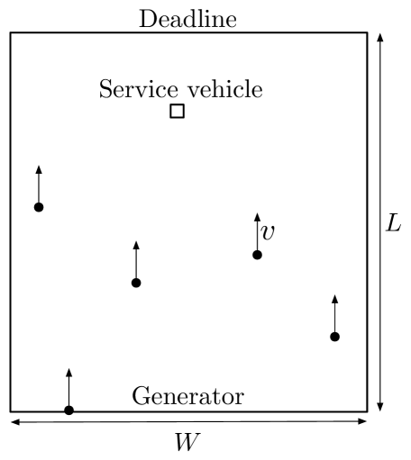
Figure 1: The problem setup. Demands are shown as black disks approaching the deadline at speed $v$. The service vehicle is a square.

We assume that the arrival process is uniform along the line segment and temporally Poisson with rate $\lambda$. In the case when the demands are faster than the service vehicle (i.e., $v\geq 1$) we introduce the novel Longest Path policy, which is based on computing longest paths in a directed acyclic reachability graph. When $L\geq vW$, we derive a lower bound on the capture fraction as a function of the system parameters. We show that the Longest Path policy is the optimal policy when $L$ is much greater than $vW$. In the case when the demands are slower than the service vehicle (i.e, $v<1$), we propose a policy based on the translational minimum Hamiltonian path called the TMHP-fraction policy. In the limit of low demand speed and high arrival rate, the capture fraction of this policy is within a small constant factor of the optimal. We present numerical simulations which verify our results, and show that the Longest Path policy performs very near the optimal even when $L<vW$.

The paper is organized as follows. In Section II we formulate the problem and in Section III we review some background material. In Section IV we consider the case of $v\geq 1$ and introduce the Longest Path Policy. In Section V we study $v<1$ and introduce the TMHP-fraction policy. Finally, in Section VI we present simulations results.

II Problem Formulation

Consider an environment $\mathcal{E}:=[0,W]\times[0,L]\subset{\mathbb{R}}^{2}$ as shown in Figure 1. The line segment $[0,W]\times\{0\}\subset\mathcal{E}$ is termed the generator, and the segment $[0,W]\times\{L\}\subset\mathcal{E}$ is termed the deadline. The environment contains a single vehicle with position $\mathbf{p}(t)=[X(t),Y(t)]^{T}\in\mathcal{E}$, modeled as a first-order integrator with unit speed. Demands (or targets) arrive in the environment according to a temporal Poisson process with rate $\lambda>0$. Upon arrival, each demand assumes a uniformly distributed location on the generator, and then moves with constant speed $v>0$ in the positive $y$-direction towards the deadline. If the vehicle intercepts a demand before the demand reaches the deadline, then the demand is captured. On the other hand, if the demand reaches the deadline before being intercepted by the vehicle, then the demand escapes. Thus, to capture a demand, it must be intercepted within $L/v$ time units of being generated.

We let $\mathcal{Q}(t)\subset\mathcal{E}$ denote the set of all outstanding demand locations at time $t$. If the $i$th demand to arrive is captured, then it is removed from $\mathcal{Q}$ and placed in the set $\mathcal{Q}_{\textup{capt}}$ with cardinality $n_{\textup{capt}}$. If the $i$th demand escapes, then it is removed from $\mathcal{Q}$ and placed in $\mathcal{Q}_{\textup{esc}}$ with cardinality $n_{\textup{esc}}$.

Causal Policy

A causal feedback control policy for the vehicle is a map $\mathcal{P}:\mathcal{E}\times\mathbb{F}(\mathcal{E})\rightarrow{\mathbb{R}}^{2}$, where $\mathbb{F}(\mathcal{E})$ is the set of finite subsets of $\mathcal{E}$, assigning a commanded velocity to the service vehicle as a function of the current state of the system: $\dot{\mathbf{p}}(t)=\mathcal{P}(\mathbf{p}(t),\mathcal{Q}(t))$.

Non-causal Policy

In a non-causal feedback control policy the commanded velocity of the service vehicle is a function of the current and future state of the system. Such policies are not physically realizable, but they will prove useful in the upcoming analysis.

Formally, let the generation of demands commence at time $t=0$, and consider the sequence of demands $(q_{1},q_{2},\ldots)$ arriving at increasing times $(t_{1},t_{2},\ldots)$, with $x$-coordinates $(x_{1},x_{2},\ldots)$. We can also model the arrival process by assuming that at time $t=0$, all demands are located in $[0,W]\times(-\infty,0]$, move in the $y$-direction at speed $v$ for all $t>0$, and are revealed to the service vehicle when they cross the generator. Thus, at time $t=0$, the position of the $i$th demand is $(x_{i},v(t-t_{i}))$. We can define a set containing the position of all demands in the region $[0,W]\times(-\infty,0]$ at time $t$ as $\mathcal{Q}_{\mathrm{unarrived}}(t)$. Then, a non-causal policy is one for which $\dot{\mathbf{p}}(t)=\mathcal{P}(\mathbf{p}(t),\mathcal{Q}(t)\cup\mathcal{Q}_{\mathrm{unarrived}}(t))$.

Problem Statement

The goal in this paper is to find causal policies $P$ that maximize the fraction of demands that are captured ${\mathbb{F}}_{\textup{cap}}(P)$, termed the capture fraction, where

$${\mathbb{F}}_{\textup{cap}}(P):=\limsup_{t\to+\infty}\mbox{$\mathbb{E}\left[\frac{n_{\textup{capt}}(t)}{n_{\textup{capt}}(t)+n_{\textup{esc}}(t)}\right]$}.$$

III Preliminary Combinatorial Results

We now review the longest path problem, the distribution of demands in an unserviced region, and optimal tours/paths through a set of points.

III-A Longest Paths in Directed Acyclic Graphs

A directed graph $G=(V,E)$ consists of a set of vertices $V$ and a set of directed edges $E\subset V\times V$. An edge $(v,w)\in E$ is directed from vertex $v$ to vertex $w$. A path in $G$ is a sequence of vertices such that from each vertex in the sequence, there is an edge in $E$ directed to the next vertex in the sequence. A path is simple if it contains no repeated vertices. A cycle is a path in which the first and last vertex in the sequence are the same. A graph $G$ is acyclic if it contains no cycles. The longest path problem is to find a simple path of maximum length (i.e., a path that visits a maximum number of vertices). In general this problem is NP-hard as its solution would imply a solution to the well known Hamiltonian path problem [14]. However, if the graph is a DAG, then the longest path problem has an efficient dynamic programming solution [1] with complexity $O(|V|+|E|)$, that relies on topologically sorting [15] the vertices.

III-B Distribution of Demands in an Unserviced Region

Demands arrive uniformly on the generator, according to a Poisson process with rate $\lambda$. The following lemma describes the distribution of demands in an unserviced region. For a finite set $\mathcal{Q}$, we let $|\mathcal{Q}|$ denote its cardinality.

Lemma III.1 (Distribution of outstanding demands, [13])

Suppose the generation of demands commences at time $0$ and no demands are serviced in the interval $[0,t]$. Let $\mathcal{Q}$ denote the set of all demands in $[0,W]\times[0,vt]$ at time $t$. Then, given a measurable compact region $\mathcal{R}$ of area $A$ contained in $[0,W]\times[0,vt]$,

$$\mathbb{P}[|\mathcal{R}\cap\mathcal{Q}|=n]=\frac{\mathrm{e}^{-\bar{\lambda}A}(\bar{\lambda}A)^{n}}{n!},\quad\text{where }\bar{\lambda}:=\lambda/(vW).$$

The previous lemma tells us that number of demands $N$ in an serviced region of area $A$ is a Poisson distributed with parameter $\lambda A/(vW)$. In addition, conditioned on $N$, the demands are independently and uniformly distributed.

III-C The Euclidean Shortest Path/Tour Problems

Given a set $\mathcal{Q}$ of $n$ points in ${\mathbb{R}}^{2}$, the Euclidean traveling salesperson problem (ETSP) is to find the minimum-length tour (i.e., cycle) of $\mathcal{Q}$. Letting $\textup{ETSP}(\mathcal{Q})$ denote the minimum length of a tour of $\mathcal{Q}$, we can state the following result.

Theorem III.2 (Length of ETSP tour, [16])

Consider a set $\mathcal{Q}$ of $n$ points independently and uniformly distributed in a compact set $\mathcal{E}$ of area $|\mathcal{E}|$. Then, there exists a constant $\beta_{\mathrm{TSP}}$ such that, with probability one,

$$\lim_{n\rightarrow+\infty}\frac{\textup{ETSP}(\mathcal{Q})}{\sqrt{n}}=\beta_{\mathrm{TSP}}\sqrt{|\mathcal{E}|}.$$ (1)

The constant $\beta_{\mathrm{TSP}}$ has been estimated numerically as $\beta_{\mathrm{TSP}}\approx 0.7120\pm 0.0002$, [17].

The Euclidean Minimum Hamiltonian Path (EMHP) problem is to compute the shortest path through a set of points. In this paper we consider a constrained EMHP problem: Given a start point $\mathbf{s}$, a set of $n$ points $\mathcal{Q}$, and a finish point $\mathbf{f}$, all in ${\mathbb{R}}^{2}$, determine the shortest path which starts at $\mathbf{s}$, visits each point in $\mathcal{Q}$ exactly once, and terminates at $\mathbf{f}$. We let $\textup{EMHP}(\mathbf{s},\mathcal{Q},\mathbf{f})$ denote the length of the shortest path.

Corollary III.3 (Length of EMHP)

Consider a set $\mathcal{Q}$ of $n$ points independently and uniformly distributed in a compact set $\mathcal{E}$ of area $|\mathcal{E}|$, and any two points $\mathbf{s},\mathbf{f}\in\mathcal{E}$. Then with probability one,

$$\lim_{n\to+\infty}\frac{\textup{EMHP}(\mathbf{s},\mathcal{Q},\mathbf{f})}{\sqrt{n}}=\beta_{\mathrm{TSP}}\sqrt{|\mathcal{E}|},$$

where $\beta_{\mathrm{TSP}}$ is defined in Theorem III.2.

The above corollary states that the length of the EMHP and the ETSP tour are asymptotically equal, and it follows directly from the fact that as $n\to+\infty$, the diameter of $\mathcal{E}$ is negligible when compared to the length of the tour/path.

III-D Translational Minimum Hamiltonian Path (TMHP)

The TMHP problem is posed as follows. Given initial coordinates; $\mathbf{s}$ of a start point, $\mathcal{Q}:=\{\mathbf{q}_{1},\dots,\mathbf{q}_{n}\}$ of a set of points, and $\mathbf{f}$ of a finish point, all moving with speed $v\in]0,1[$ in the positive $y$-direction, determine a minimum length path that starts at time zero from point $\mathbf{s}$, visits all points in the set $\mathcal{Q}$ and ends at the finish point. The following gives a solution [4] for the TMHP problem.
(i) Define the map $\operatorname{g}:{\mathbb{R}}^{2}\rightarrow{\mathbb{R}}^{2}$ by

$$\operatorname{g}(x,y)=\Big{(}\frac{x}{\sqrt{1-v^{2}}},\frac{y}{1-v^{2}}\Big{)}.$$

(ii) Compute the EMHP that starts at $\operatorname{g}_{v}(\mathbf{s})$, passes through $\{\operatorname{g}(\mathbf{q}_{1}),\dots,\operatorname{g}(\mathbf{q}_{n})\}=:\operatorname{g}(\mathcal{Q})$ and ends at $\operatorname{g}(\mathbf{f})$.
(iii) To reach a translating point with initial position $(x,y)$ from the initial position $(X,Y)$, move towards the point $(x,y+vT)$, where

$$T=\frac{\sqrt{(1-v^{2})(X-x)^{2}+(Y-y)^{2}}}{1-v^{2}}-\frac{v(Y-y)}{1-v^{2}}.$$

The length $\textup{TMHP}_{v}(\mathbf{s},\mathcal{Q},\mathbf{f})$ of the path is as follows.

Lemma III.4 (TMHP length, [4])

Let the initial coordinates $\mathbf{s}=(x_{\mathbf{s}},y_{\mathbf{s}})$ and $\mathbf{f}=(x_{\mathbf{f}},y_{\mathbf{f}})$, and the speed of the points $v\in{]0,1[}$. Then,

$$\textup{TMHP}_{v}(\mathbf{s},\mathcal{Q},\mathbf{f})=\textup{EMHP}(\operatorname{g}(\mathbf{s}),\operatorname{g}(\mathcal{Q}),\operatorname{g}(\mathbf{f}))+\frac{v(y_{\mathbf{f}}-y_{\mathbf{s}})}{1-v^{2}}.$$

IV Demand Speed Greater Than Vehicle Speed

Here we develop a policy for the case when the demand speed $v\geq 1$. In this policy, the service vehicle remains on the deadline and services demands as per the longest path in a directed acyclic reachability graph. In this section we begin by introducing the reachability graph, and then proceed to state and analyze the Longest Path policy.

IV-A Reachable Demands

Consider a demand generated at time $t_{1}\geq 0$ at position $(x,0)$. The demand moves in the positive $y$-direction at speed $v\geq 1$, and thus $(x(t),y(t))=(x,v(t-t_{1}))$ for each $t\in[t_{1},T]$, where $T$ is either the time of escape (i.e., $T=L/v+t_{1}$), or it is the time of capture. Now, given the service vehicle location $(X(t),Y(t))$, a demand with position $(x,y(t))$ is reachable if and only if

$$v|X(t)-x|\leq Y(t)-y(t).$$ (2)

That is, the service vehicle must be at a height of at least $v|X(t)-x|$ above the demand in order to capture it.

Definition IV.1 (Reachable set)

The reachable set from a position $(X,Y)\in\mathcal{E}$ is

$$R(X,Y):=\{(x,y)\in\mathcal{E}:v|X-x|\leq|Y-y|\}.$$

If the service vehicle is located at $(X,Y)$, then a demand can be captured if and only if it lies in the set $R(X,Y)$.

An example of the reachable set is shown in Figure 2.

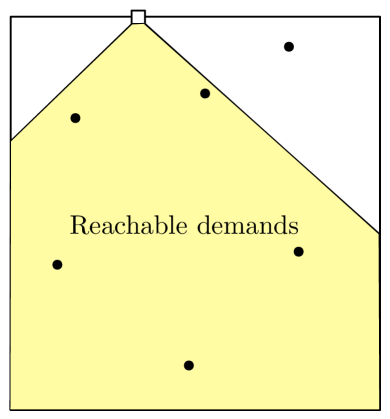
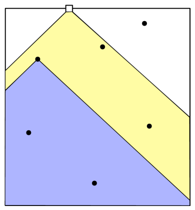
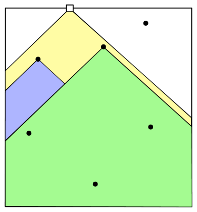
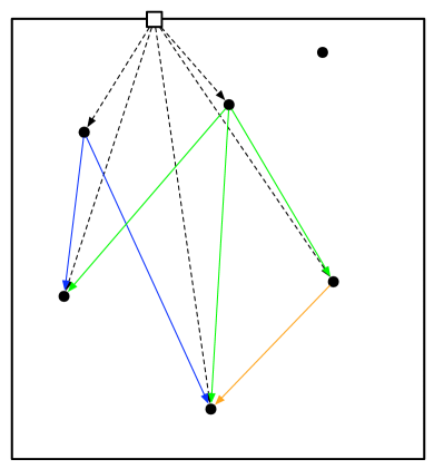
Figure 2: The construction of the reachability graph. The top-left figure shows the set of reachable points from a vehicle positioned on the deadline. The top-right and bottom-left figures show the reachable set from demand locations. The bottom-right figure shows the reachability graph.

Next, given a demand in the reachable set, the following motion gives a method of capture.

Definition IV.2 (Intercept motion)

Consider a vehicle position $((X(\bar{t}),Y(\bar{t}))$ and a demand position $(x,y(\bar{t}))\in R(X(\bar{t}),Y(\bar{t}))$ at time $\bar{t}\geq 0$. In intercept motion, the service vehicle captures the demand by first moving horizontally at unit speed to the position $(x_{i},Y(\bar{t}))$, and then waiting at the location for the demands arrival.

Lemma IV.3 (Optimality of intercept motion)

Consider $v\geq 1$, and let the service vehicle be initially positioned on the deadline. Then, there is an optimal policy in which the service vehicle uses only intercept motion.

Proof: Let the service vehicle be positioned at $(X,L)$, and consider a demand at $(x,y)\in R(X,L)$. From equation (2), we have $v|X-x|\leq L-y$. If $v|X-x|=L-y$, then deadline motion is the only way in which the demand can be captured. Thus, assume that $v|X-x|<L-y$, and consider two cases; Case 1 in which intercept motion is used, and Case 2 in which the demand is captured at a location $(x,Y)$, where $Y<L$.

Notice that the position of each outstanding demand relative to the service vehicle position at capture is the same in Case 1 as in Case 2. Thus, the reachable set in Case 2 is a strict subset of reachable set in Case 1 and the vehicle gains no advantage by moving off of the deadline.   

Next, consider the set of demands in $R(X(\bar{t}),Y(\bar{t}))$, and suppose the vehicle chooses to capture demand $i$, with position $\mathbf{q}_{i}(\bar{t})=(x_{i},y_{i}(\bar{t}))\in R(X(\bar{t}),Y(\bar{t}))$. Upon capture at time $T$, the service vehicle can recompute the reachable set, and select a demand that lies within. Since all demands translate together, every demand that was reachable from $\mathbf{q}_{i}(\bar{t})$, is reachable from $\mathbf{q}_{i}(T)$. Thus, the service vehicle can “look ahead” and compute the demands that will be reachable from each captured demand position. This idea motivates the concept of a reachability graph.

Definition IV.4 (Reachability graph)

For $v\geq 1$, the reachability graph of a set of points $\{\mathbf{q}_{1},\ldots,\mathbf{q}_{n}\}\in\mathcal{E}$, is a directed acyclic graph with vertex set $V:=\{1,\ldots,n\}$, and edge set $E$, where for $i,j\in V$, the edge $(i,j)$ is in $E$ if and only if $\mathbf{q}_{j}\in R(\mathbf{q}_{i})$ and $j\neq i$.

Given a set $\mathcal{Q}$ of $n$ outstanding demands, and a vehicle position $(X,Y)$, we can compute the corresponding reachability graph (see Fig. 2) in $O(n^{2})$ computation time. In addition, by Section III-A we can compute the longest path in a reachability graph in $O(n^{2})$ computation time.

IV-B A Non-causal Policy and Upper Bound

To derive an upper bound for $v\geq 1$, we begin by considering a non-causal policy. In the online algorithms literature, such a policy would be referred to as an offline algorithm [9]. Figure 3 shows an example of a path generated by the Non-causal Longest Path policy. Note that the service vehicle will intercept each demand on the deadline, and thus the path depicts which demands will be captured, and in what order.

Assumes: Vehicle is located on deadline and $v\geq 1$.

Compute the reachability graph of the vehicle position and all demands in $\mathcal{Q}(0)\cup\mathcal{Q}_{\mathrm{unarrived}}(0)$.

Compute a longest path in this graph, starting at the service vehicle location.

Capture demands in the order they appear on the path, intercepting each demand on the deadline.

Algorithm 1 Non-causal Longest Path (NCLP) policy

3

3

3

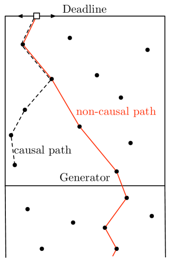
Figure 3: A snapshot in the evolution of the Non-causal Longest Path policy. The vehicle has planned the solid red path through all demands, including those that have not yet arrived. In comparison, a dashed causal longest path is shown, which only considers demands that have arrived.

Lemma IV.5 (Optimal non-causal policy)

If $v\geq 1$, then the Non-causal Longest Path policy is an optimal non-causal policy. Moreover, if $v\geq 1$, then for every causal policy $P$,

$${\mathbb{F}}_{\textup{cap}}(P)\leq{\mathbb{F}}_{\textup{cap}}(\mathrm{NCLP}).$$

Proof: The reachability graph $\mathcal{Q}(0)\cup\mathcal{Q}_{\mathrm{unarrived}}(0)$ contains every possible path that the service vehicle can follow. When $v\geq 1$ the graph is a directed acyclic graph and thus the longest path (i.e., the path which visits the most vertices in the graph) is well defined. The vehicle uses intercept motion, and thus by Lemma IV.3 the NCLP policy is an optimal non-causal policy, and its capture fraction upper bounds every causal policy.   

IV-C The Longest Path Policy

We now introduce the Longest Path policy. In the LP policy, the fraction $\eta$ is a design parameter. The lower $\eta$ is chosen, the better the performance of the policy, but this comes at the expense of increased computation.

Assumes: Vehicle is located on deadline and $v\geq 1$

Compute the reachability graph of the vehicle position and all demands in $\mathcal{Q}(0)$.

Compute a longest path in this graph, starting at the service vehicle location.

Capture demands in the order they appear on the path, intercepting each demand on the deadline.

Once a fraction $\eta\in{]0,1]}$ of the demands on the path have been serviced, recompute the reachability graph of all outstanding demands and return to step 2.

Algorithm 2 The Longest Path (LP) policy

4

4

4

4

In the following theorem, we relate the Longest Path policy to its non-causal relative. Such a bound is referred to as a competitive ratio in the online algorithms literature [9].

Theorem IV.6 (Optimality of Longest Path policy)

If $v\geq 1$, then

$${\mathbb{F}}_{\textup{cap}}(\mathrm{LP})\geq\left(1-\frac{vW}{L}\right){\mathbb{F}}_{\textup{cap}}(\mathrm{NCLP}),$$

and thus the LP policy is optimal as $vW/L\to+\infty$.

Proof: Suppose that the generation of demands begins at $t=0$ and let us consider two scenarios; (a) the vehicle uses the Longest Path policy, and (b) the vehicle uses the Non-causal Longest Path policy. Then, at any instant in time $t_{1}>0$ we can compare the number of demands captured in scenario (a) to the number captured in scenario (b) (refer to Fig. 4).

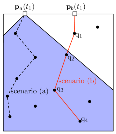
Figure 4: Scenario (a) and (b) for the proof of Theorem IV.6. Path (a) visits five demands and thus $\mathcal{L}_{a}=5$. Path (b) visits four demands, yielding $m=4$. The demand $\mathbf{q}_{2}$ is the highest on path (b) that can be captured from $\mathbf{p}_{a}(t_{1})$. Thus, $n=1$, and $5=\mathcal{L}_{a}>m-n=3$.

Let us consider a time instant $t_{1}$ where in scenario (a), the vehicle is recomputing the longest path through all outstanding demands $\mathcal{Q}(t_{1})$. Let us denote by $\mathbf{p}_{a}(t_{1})$ and $\mathbf{p}_{b}(t_{1})$, the vehicle position in scenario (a) and scenario (b), respectively, at time $t_{1}$. In scenario (b), let the path that the vehicle will take through $\mathcal{Q}(t_{1})$ be given by $(\mathbf{q}_{1},\mathbf{q}_{2},\ldots,\mathbf{q}_{m})\in\mathcal{Q}(t_{1})$. The demand $\mathbf{q}_{1}$ is reachable from $\mathbf{p}_{b}(t_{1})$, but it may not be reachable from $\mathbf{p}_{a}(t_{1})$. However, a lower bound on the length of the longest path in scenario (a) is: $(\mathbf{q}_{n+1},\mathbf{q}_{n+2},\ldots,\mathbf{q}_{m})$, where $\mathbf{q}_{n+1}$, $n\in\{0,\ldots,m-1\}$, is the highest demand that can be captured from $\mathbf{p}_{a}(t_{1})$, see Fig. 4. Thus, the length of the longest path in scenario (a), $\mathcal{L}_{a}$, is at least

$$\mathcal{L}_{a}\geq m-n,$$ (3)

where $m$ is the length of the path in scenario (b).

Now, since the deadline has width $W$, the vehicle in scenario (a) can capture any demand $(x,y)$ with $y\leq L-vW$. Thus, the demands $\mathbf{q}_{1},\ldots,\mathbf{q}_{n}$ must all have $y$-coordinates in ${]L-vW,L]}$. Let the total number of outstanding demands at time $t_{1}$ be ${N}_{\textup{tot}}$. Then, conditioned on ${N}_{\textup{tot}}$, by Lemma III.1, the expected number of outstanding demands contained in $[0,W]\times{]L-vW,L]}$ is ${N}_{\textup{tot}}vW/L$. Hence,

$$\mbox{$\mathbb{E}\left[n|{N}_{\textup{tot}}\right]$}={N}_{\textup{tot}}\frac{vW}{L}{\mathbb{F}}_{\textup{cap}}(\mathrm{NCLP}).$$ (4)

Similarly, for the length of the path through $\mathcal{Q}(t_{1})$ in scenario (b), we have

$$\mbox{$\mathbb{E}\left[m|{N}_{\textup{tot}}\right]$}={N}_{\textup{tot}}{\mathbb{F}}_{\textup{cap}}(\mathrm{NCLP}).$$ (5)

Combining equations (4) and (5) with equation (3) we obtain

$$\mathbb{E}\left[\mathcal{L}_{a}|{N}_{\textup{tot}}\right] \geq{N}_{\textup{tot}}\left(1-\frac{vW}{L}\right){\mathbb{F}}_{\textup{cap}}(\mathrm{NCLP}),$$

$$\mathbb{E}\left[\frac{\mathcal{L}_{a}}{{N}_{\textup{tot}}}|{N}_{\textup{tot}}\right] \geq\left(1-\frac{vW}{L}\right){\mathbb{F}}_{\textup{cap}}(\mathrm{NCLP}).$$

But $\mathcal{L}_{a}/{N}_{\textup{tot}}$ is the fraction of outstanding demands in $\mathcal{Q}(t_{1})$ that will be captured in scenario (a), and it does not depend on the value of ${N}_{\textup{tot}}$. By the law of total expectation

$$\mbox{$\mathbb{E}\left[\frac{\mathcal{L}_{a}}{{N}_{\textup{tot}}}\right]$}=\mbox{$\mathbb{E}\left[\mbox{$\mathbb{E}\left[\frac{\mathcal{L}_{a}}{{N}_{\textup{tot}}}|{N}_{\textup{tot}}\right]$}\right]$}\geq\left(1-\frac{vW}{L}\right){\mathbb{F}}_{\textup{cap}}(\mathrm{NCLP}).$$

Each time the longest path is recomputed, the path in scenario (a) will capture at least this fraction of demands. Thus, we have ${\mathbb{F}}_{\textup{cap}}(\mathrm{LP})\geq\mbox{$\mathbb{E}\left[\mathcal{L}_{a}/{N}_{\textup{tot}}\right]$}$ and have proved the result.   

Remark IV.7 (Conservativeness of bound)

The bound in Theorem IV.6 is conservative. This is primarily due to bounding the expected distance between the causal and non-causal paths by $W$. The distance between two independently and uniformly distributed points in $[0,W]$, is $W/3$. The distance is even less if the points are positively correlated (as is likely the case for the distance between paths). Thus, it seems that it may be possible to increase the bound to

$${\mathbb{F}}_{\textup{cap}}(\mathrm{LP})\geq\left(1-\frac{vd}{L}\right){\mathbb{F}}_{\textup{cap}}(\mathrm{NCLP}),$$

where $d<W/3$. $\square$

The previous theorem establishes the performance of the Longest Path policy relative to a non-causal policy. However, the LP policy is difficult analyze directly. This is due to the fact that the position of the vehicle at time $t$ depends on the positions of all outstanding demands in $\mathcal{Q}(t)$. Thus, our approach is to lower bound the capture fraction of the LP policy with a greedy policy:

Assumes: Vehicle is located at $(X,L)$

Compute the reachability set $R(X,L)$.

Capture the demand in $R(X,L)$ with the highest $y$-coordinate using intercept motion.

Repeat.

Algorithm 3 The Greedy Path (GP) policy

3

3

3

Given a set of outstanding demands $\mathcal{Q}(t)$ at time $t$, the Greedy Path policy generates a suboptimal longest path through $\mathcal{Q}(t)$. In addition, the vehicle position is independent of all outstanding demands, except the demand currently being captured. Thus, the capture fraction of the Greedy Path policy provides a lower bound for the capture fraction of the Longest Path policy. We are now able to establish the following result.

Theorem IV.8 (Lower Bound for Longest Path policy)

If $L\geq vW$, then for the Longest Path policy

$${\mathbb{F}}_{\textup{cap}}(\mathrm{LP})\geq{\mathbb{F}}_{\textup{cap}}(\mathrm{GP})\geq\frac{1}{\sqrt{\pi\alpha}\operatorname{erf}(\sqrt{\alpha})+\mathrm{e}^{-\alpha}},$$

where $\alpha=\lambda W/2$ and $\operatorname{erf}:{\mathbb{R}}\to[-1,1]$ is the error function.

Proof: We begin by looking at the expression for the capture fraction. Notice that if $n_{\textup{capt}}(t)>0$ for some $t>0$, then

$$\limsup_{t\to+\infty}\mbox{$\mathbb{E}\left[\frac{n_{\textup{capt}}(t)}{n_{\textup{capt}}(t)+n_{\textup{esc}}(t)}\right]$} =\limsup_{t\to+\infty}\mbox{$\mathbb{E}\left[\frac{1}{1+\frac{n_{\textup{esc}}(t)}{n_{\textup{capt}}(t)}}\right]$}$$ (6)

$$\geq\left(1+\limsup_{t\to+\infty}\mbox{$\mathbb{E}\left[\frac{n_{\textup{esc}}(t)}{n_{\textup{capt}}(t)}\right]$}\right)^{-1},$$

where the last step comes from an application of Jensen’s inequality [18]. Thus, we can determine a lower bound on the capture fraction by studying the number of demands that escape per captured demand.

Let us study the time instant $t$ at which the service vehicle captures its $i$th demand, and determine an upper bound on the number of demands that escape before the service vehicle captures its $(i+1)$th demand. Since we seek a lower bound on the capture fraction of the LP policy, we may consider the path generated by the Greedy Path policy. In addition, we consider the worst-case service vehicle position; namely, the position $(0,L)$ (or equivalently $(W,L)$).

From the position $(0,L)$, the reachable set is

$$R(0,L)=\{(x,y)\in\mathcal{E}:vx\leq L\}.$$

Let $R_{y}$ denote the reachable set intersected with $[0,W]\times[L-y,L]$, where $y\in[0,L]$, and let $|R_{y}|$ denote its area. Then,

$$|R_{y}|=\begin{cases}\frac{y^{2}}{2v},&\text{if $y\leq vW$},\\ yW-\frac{vW^{2}}{2},&\text{if $y>vW$}.\end{cases}$$

An illustration of the set $R_{y}$ is shown in Figure 5.

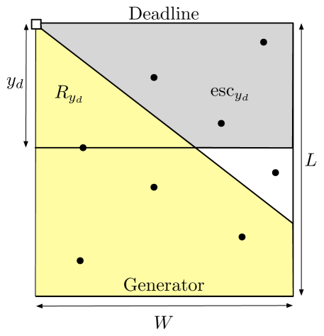
Figure 5: The setup for the proof of Theorem IV.8. The service vehicle is located at $(0,L)$. All demands in the region $\textup{esc}_{y_{d}}$ escape while capturing the demand with the highest $y$-coordinate.

Let $y_{d}$ be the $y$-distance to the reachable demand with the highest $y$-coordinate. That is,

$$y_{d}=\min_{(x,y)\in\mathcal{Q}(t)\cap R(0,L)}\{L-y\},$$

where $\mathcal{Q}(t)$ is the set of outstanding demands at time $t$. By Lemma III.1, the probability that a subset $\mathcal{B}\subset\mathcal{E}$ with area $|\mathcal{B}|$ contains zero demands is given by

$$\mathbb{P}[|\mathcal{B}\cap\mathcal{Q}(t)|=0]=\mathrm{e}^{-\lambda|\mathcal{B}|/(vW)},$$

where $|\mathcal{B}\cap\mathcal{Q}(t)|$ denotes the cardinality of the finite set $\mathcal{B}\cap\mathcal{Q}(t)$. Thus,

$$\mathbb{P}[y_{d}>y]=\mathbb{P}[|R_{y}\cap\mathcal{Q}(t)|=0]=\mathrm{e}^{-\lambda|R_{y}|/(vW)}.$$

The probability density function of $y_{d}$ for $y_{d}\leq vW$ is

$$f(y)=\frac{d}{dy}(1-\mathbb{P}[y_{d}>y]) =\frac{d}{dy}\mathrm{e}^{-\lambda y^{2}/(2v^{2}W)}$$

$$=\frac{\lambda}{v^{2}W}y\mathrm{e}^{-\lambda y^{2}/(2v^{2}W)}.$$

Now, given $y_{d}$, all demands residing in the region $\textup{esc}_{y_{d}}:=([0,W]\times[L-y_{d},L])\setminus R_{y_{d}}$ will escape (see Fig. 5). The area of $\textup{esc}_{y_{d}}$ is

$$|\textup{esc}_{y_{d}}|=\begin{cases}y_{d}W-\frac{y_{d}^{2}}{2v},&\text{if $y_{d}\leq vW$},\\ \frac{vW^{2}}{2},&\text{if $y_{d}\geq vW$}.\end{cases}$$

From Section III-B, the expected number of outstanding demands in an unserviced region of area $A$ is $\lambda A/(vW)$. Thus, given that the vehicle is located at $(0,L)$, the expected number of demands that escape while the service vehicle is capturing its $(i+1)$th demand is given by

$$\mbox{$\mathbb{E}\left[n_{\textup{esc},i}\right]$}=\frac{\lambda}{vW}\mbox{$\mathbb{E}\left[|\textup{esc}_{y_{d}}|\right]$}$$

$$=\frac{\lambda}{vW}\left[\int_{0}^{vW}\left(yW-\frac{y^{2}}{2v}\right)f(y)dy+\frac{vW^{2}}{2}\mathbb{P}[y_{d}>vW]\right].$$

Applying the probability density function and cumulative distribution function of $y_{d}$ we obtain

$$\mbox{$\mathbb{E}\left[n_{\textup{esc},i}\right]$}=\frac{\lambda^{2}}{v^{3}W^{2}}\int_{0}^{vW}\left(yW-\frac{y^{2}}{2v}\right)y\mathrm{e}^{-\lambda y^{2}/(2v^{2}W)}dy\\ +\frac{\lambda W}{2}\mathrm{e}^{-\lambda W/2}.$$ (7)

To evaluate the integral, consider the change of coordinates $z:=y/vW$, and define $\alpha:=\lambda W/2$. After simplifying, the integral becomes

$$4\alpha^{2}\int_{0}^{1}\left(z^{2}-\frac{z^{3}}{2}\right)\mathrm{e}^{-\alpha z^{2}}dz.$$

Integrating by parts we obtain

$$\sqrt{\pi\alpha}\operatorname{erf}(\sqrt{\alpha})+\alpha\mathrm{e}^{-\alpha}+\mathrm{e}^{-\alpha}-1,$$ (8)

where $\operatorname{erf}:{\mathbb{R}}\to[-1,1]$ is the error function:

$$\operatorname{erf}(x)=\frac{2}{\pi}\int_{0}^{x}\mathrm{e}^{-t^{2}}dt.$$

Substituting equation (8) into equation (7) we obtain

$$\mbox{$\mathbb{E}\left[n_{\textup{esc},i}\right]$}=\sqrt{\pi\alpha}\operatorname{erf}(\sqrt{\alpha})+\mathrm{e}^{-\alpha}-1.$$

Since $\mathbb{E}\left[n_{\textup{esc},i}\right]$ is computed for the worst-case vehicle position $(0,L)$, and since this expression holds at every capture, we have that

$$\limsup_{t\to+\infty}\mbox{$\mathbb{E}\left[\frac{n_{\textup{esc}}(t)}{n_{\textup{capt}}(t)}\right]$}\leq\sqrt{\pi\alpha}\operatorname{erf}(\sqrt{\alpha})+\mathrm{e}^{-\alpha}-1,$$

and thus by equation (6) we obtain the desired result.   

V Demand speed less than vehicle speed

In this section we study the case when the demand speed $v<1$. For this case, an upper bound on the capture fraction has been derived in [13]. We introduce a policy which is a variant of the TMHP-based policy in [13], and lower bound its capture fraction in the limit of low demand speed and high demand arrival rate.

V-A Capture Fraction Upper Bound

The following theorem upper bounds the capture fraction of every policy for the case of $v<1$.

Theorem V.1 (Capture fraction upper bound, [13])

If $v<1$, then for every causal policy $P$

$${\mathbb{F}}_{\textup{cap}}(P)\leq\min\left\{1,\frac{2}{\sqrt{v\lambda W}}\right\}.$$

The proof of the above theorem is contained in [13], and relies on a computation of the expected minimum distance between demands. Notice that for low demands speed, i.e., $v\ll 1$, it may be possible to achieve a capture fraction of one, even for high arrival rates.

V-B The TMHP-fraction Policy

In Section III-D we reviewed the translational minimum Hamiltonian Path (TMHP) through a set of demands. The following policy utilizes this path to service demands.

Assumes: Vehicle is located on the line $y=L/2$.

Compute a translational minimum Hamiltonian path through all outstanding demands in $[0,W]\times[0,L/2]$, starting at the service vehicle position, and terminating at the demand with the lowest $y$-coordinate.

if time to travel entire path is less than $L/(2v)$ then  Service all outstanding demands by following the computed path.

else  Service outstanding demands along the computed path for $L/(2v)$ time units.

 Repeat.

Algorithm 4 The TMHP-fraction (TF) policy

3

3

3

Figure 6 shows an example of the TMHP-fraction policy. In contrast with the LP policy, where the vehicle remains on the deadline, in the TMHP-fraction policy the vehicle follows the TMHP using minimum time motion between demands as described in Section III-D.

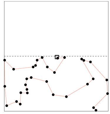
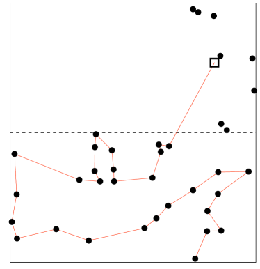
Figure 6: The TMHP-fraction policy. The left-hand figure shows a TMHP through all outstanding demands. The right-figure shows the instant when the vehicle has followed the path for $L/(2v)$ time units and recomputes its path, allowing some demands to escape.

Notice that none of the demands in the region $[0,W]\times[0,L/2]$ at time $t$ will have escaped before time $t+L/(2v)$. Thus, the vehicle is guaranteed that for the first $L/(2v)$ time units, all demands on the TMHP path are still in the environment. For the TMHP-fraction policy we have the following result.

Theorem V.2 (TMHP-fraction policy lower bound)

In the limit as $v\to 0^{+}$ and $\lambda\to+\infty$, the capture fraction of the TMHP-fraction policy satisfies

$${\mathbb{F}}_{\textup{cap}}(\mathrm{TF})\geq\min\left\{1,\frac{1}{\beta_{\mathrm{TSP}}\sqrt{v\lambda W}}\right\}.$$

Proof: Consider the beginning of an iteration of the policy, and assume that the duration of the previous iteration was $L/(2v)$. In this case, the vehicle has $y$-coordinate $Y\in[L/2,L]$, and by Lemma III.1, the region $\mathcal{R}:=[0,W]\times[0,L/2]$ contains a number of demands $N$ that is Poisson distributed with parameter $\lambda L/(2v)$. Conditioned on $N$, the demands are independently and uniformly distributed in $\mathcal{R}$.

Now, we make use of the following three facts. First, as $v\to 0^{+}$, the length of the TMHP constrained to start at the vehicle location and end at the lowest demand, is equal to the length of the EMHP in the corresponding static instance, as described in Lemma III.4. Second, from Corollary III.3, for uniformly distributed points, the asymptotic length of a constrained EMHP is equal to the asymptotic length of the ETSP tour. Third, as $v\to 0^{+}$, and $\lambda\to+\infty$, we have that $N$ tends to $+\infty$ with probability one. Using the above facts we obtain that the length of the TMHP starting at the vehicle position, passing through all demands in $\mathcal{R}$, and terminating at the demand with the lowest $y$-coordinate, has length $\beta_{\mathrm{TSP}}\sqrt{NWL/2}$ in the limiting regime as $v\to 0^{+}$, and $\lambda\to+\infty$.

The vehicle will follow the TMHP for at most $L/(2v)$ time units, and thus will service $cN$ demands, where

$$c=\min\left\{1,\frac{\sqrt{L}}{\beta_{\mathrm{TSP}}v\sqrt{2NW}}\right\}.$$

Now, the random variable $N$ has expected value $\mbox{$\mathbb{E}\left[N\right]$}=\lambda L/(2v)$ and variance $\sigma^{2}_{N}=\lambda L/(2v)$. By the Chebyshev inequality, $\mathbb{P}[|N-\mbox{$\mathbb{E}\left[N\right]$}|\geq\alpha]\leq\sigma^{2}_{N}/\alpha^{2}$, and thus letting $\alpha=\sqrt{v}\mbox{$\mathbb{E}\left[N\right]$}$, we have

$$\mathbb{P}[N\geq(1+\sqrt{v})\mbox{$\mathbb{E}\left[N\right]$}]\leq\frac{1}{v\mbox{$\mathbb{E}\left[N\right]$}}=\frac{2}{\lambda L}.$$

Thus, we have

$$c\geq\min\left\{1,\frac{1}{\beta_{\mathrm{TSP}}\sqrt{(1+\sqrt{v})v\lambda W}}\right\}.$$

with probability at least $1-2/(\lambda L)$. In the limit as $\lambda\to+\infty$, with probability 1,

$$c\geq\min\left\{1,\frac{1}{\beta_{\mathrm{TSP}}\sqrt{v\lambda W}}\right\}.$$ (9)

Therefore, if the previous iteration had duration at least $L/(2v)$, then the total fraction of demands captured in the current iteration is given by equation (9).

The other case is that the previous iteration had duration $T<L/(2v)$. In this case, all outstanding demands in the region $\mathcal{R}:=[0,W]\times[0,L/2]$ lie in a subset $[0,W]\times[0,vT]$, and the subset contains a number of demands $N$ that is Poisson distributed with parameter $\lambda T\leq\lambda L/(2v)$. Thus, in this case there are fewer outstanding demands, and the bound on $c$ still holds. Thus, ${\mathbb{F}}_{\textup{cap}}(\mathrm{TF})\geq c$, and we obtain the desired result.   

Remark V.3 (Bound comparison)

In the limit as $v\to 0^{+}$, and $\lambda\to+\infty$, the capture fraction of the TMHP-fraction policy is within a factor of $2\beta_{\mathrm{TSP}}\approx 1.42$ of the optimal. $\square$

VI Simulations

We now present two sets of results from numerical experiments. The first set compares the Longest Path policy with $\eta=1$ to the Non-causal Longest Path policy and to the theoretical lower bound in Theorem IV.8. The second set compares the TMHP-fraction policy to the policy independent upper bound in Theorem V.1 and the lower bound in Theorem V.2.

To simulate the LP and the NCLP policies, we perform $10$ runs of the policy, where each run consists of $5000$ demands. A comparison of the capture fractions for the two policies is presented in Figure 7. When $L>vW$, the capture fraction of the LP policy is nearly identical to that of the NCLP policy. Even in Figure 7(a), where $L<vW$, the capture fraction of the LP policy is within $2\%$ of the NCLP policy, and thus the optimal. This suggests that the Longest Path policy is essentially optimal over a large range of parameter values.

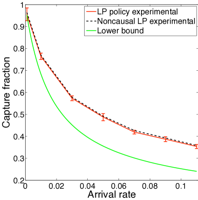
(a) $v=2$ and $L>vW$.

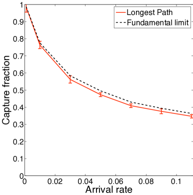
(b) $v=5$ and $L<vW$.

Figure 7: Simulation results for LP policy (solid red line with error bars showing $\pm$ one standard deviation) and the NCLP policy (dashed black line) for an environment of width $W=120$ and length $L=500$. In (a), $L>vW$, and the lower bound in Theorem IV.8 is shown in solid green.

To simulate the TMHP-fraction policy, the linkern solver is used to generate approximations to the optimal TMHP. For each value of arrival rate, we determine the capture fraction by taking the mean over $10$ runs of the policy. A comparison of the simulation results with the theoretical results from Section V are presented in Figure 8.

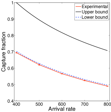
(a) Demand speed $v=0.01$.

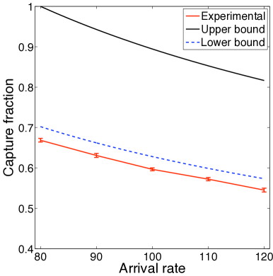
(b) Demand speed $v=0.05$.

Figure 8: Simulation results for TMHP-fraction policy. The solid black curve shows the upper bound in Theorem V.1 and the dashed line shows the lower bound in Theorem V.2. Numerical results are shown with error bars.

For $v=0.01$ in Fig. 8(a), the experimental results are in near exact agreement with the theoretical lower bound in Theorem V.1. For $v=0.05$ in Fig. 8(b), the experimental results are within $5\%$ of the theoretical lower bound. However, notice that the experimental capture fraction is smaller than the theoretical lower bound. This is due to several factors. First, we have not reached the limit as $v\to 0^{+}$ and $\lambda\to+\infty$ where the asymptotic value of $\beta_{\mathrm{TSP}}\approx 0.712$ holds. Second, we are using an approximate solution to the optimal TMHP, generated via the linkern solver.

VII Conclusions

In this paper we introduced a pursuit problem in which a vehicle must guard a deadline from approaching demands. We presented novel policies in the case when the demand speed is greater than the vehicle speed, and in the case when the demand speed is less than the vehicle speed. In the former case we introduced the Longest Path policy which is based on computing longest paths in the directed acyclic reachability graph, and in the latter case we introduced the TMHP-fraction policy. For each policy, we analyzed the fraction of demands that are captured.

There are many areas for future work. The Longest Path policy has promising extensions to the case when demands have different priority levels, and to the case of multiple vehicles. We would also like to fully characterize the capture fraction when $L<vW$, and tighten our existing bounds to reflect the near optimal performance shown in simulation.

References

- [1] N. Christofides, Graph Theory: An Algorithmic Approach. Academic Press, 1975.
- [2] N. Bansal, A. Blum, S. Chawla, and A. Meyerson, “Approximation algorithms for deadline-TSP and vehicle routing with time-windows,” in ACM Symposium on the Theory of Computing, Chicago, IL, 2004, pp. 166 – 174.
- [3] P. Chalasani and R. Motwani, “Approximating capacitated routing and delivery problems,” SIAM Journal on Computing, vol. 28, no. 6, pp. 2133–2149, 1999.
- [4] M. Hammar and B. J. Nilsson, “Approximation results for kinetic variants of TSP,” Discrete and Computational Geometry, vol. 27, no. 4, pp. 635–651, 2002.
- [5] C. S. Helvig, G. Robins, and A. Zelikovsky, “The moving-target traveling salesman problem,” Journal of Algorithms, vol. 49, no. 1, pp. 153–174, 2003.
- [6] Y. Asahiro, E. Miyano, and S. Shimoirisa, “Grasp and delivery for moving objects on broken lines,” Theory of Computing Systems, vol. 42, no. 3, pp. 289–305, 2008.
- [7] H. N. Psaraftis, “Dynamic vehicle routing problems,” in Vehicle Routing: Methods and Studies, B. Golden and A. Assad, Eds. Elsevier (North-Holland), 1988, pp. 223–248.
- [8] D. J. Bertsimas and G. J. van Ryzin, “A stochastic and dynamic vehicle routing problem in the Euclidean plane,” Operations Research, vol. 39, pp. 601–615, 1991.
- [9] A. Borodin and R. El-Yaniv, Online Computation and Competitive Analysis. Cambridge University Press, 1998.
- [10] S. O. Krumke, W. E. de Paepe, D. Poensgen, and L. Stougie, “News from the online traveling repairmain,” Theoretical Computer Science, vol. 295, no. 1-3, pp. 279–294, 2003.
- [11] M. Pavone, N. Bisnik, E. Frazzoli, and V. Isler, “A stochastic and dynamic vehicle routing problem with time windows and customer impatience,” ACM/Springer Journal of Mobile Networks and Applications, 2008, to appear. [Online]. Available: http://ares.lids.mit.edu/papers/Pavone.Bisnik.ea.MONE08.pdf
- [12] S. L. Smith, M. Pavone, F. Bullo, and E. Frazzoli, “Dynamic vehicle routing with priority classes of stochastic demands,” SIAM Journal on Control and Optimization, Feb. 2009, submitted.
- [13] S. D. Bopardikar, S. L. Smith, F. Bullo, and J. P. Hespanha, “Dynamic vehicle routing for translating demands: Stability analysis and receding-horizon policies,” IEEE Transactions on Automatic Control, Mar. 2009, submitted.
- [14] B. Korte and J. Vygen, Combinatorial Optimization: Theory and Algorithms, 4th ed., ser. Algorithmics and Combinatorics. Springer, 2007, vol. 21.
- [15] T. H. Cormen, C. E. Leiserson, R. L. Rivest, and C. Stein, Introduction to Algorithms, 2nd ed. MIT Press, 2001.
- [16] J. Beardwood, J. Halton, and J. Hammersly, “The shortest path through many points,” in Proceedings of the Cambridge Philosophy Society, vol. 55, 1959, pp. 299–327.
- [17] A. G. Percus and O. C. Martin, “Finite size and dimensional dependence of the Euclidean traveling salesman problem,” Physical Review Letters, vol. 76, no. 8, pp. 1188–1191, 1996.
- [18] L. Breiman, Probability, ser. Classics in Applied Mathematics. SIAM, 1992, vol. 7, corrected reprint of the 1968 original.