An Intensive HST  Survey for $z>1$ Type Ia Supernovae by Targeting Galaxy Clusters

Abstract

We present a new survey strategy to discover and study high redshift Type Ia supernovae (SNe Ia) using the Hubble Space Telescope (HST). By targeting massive galaxy clusters at $0.9<z<1.5$, we obtain a twofold improvement in the efficiency of finding SNe compared to an HST field survey and a factor of three improvement in the total yield of SN detections in relatively dust-free red-sequence galaxies. In total, sixteen SNe were discovered at $z>0.95$, nine of which were in galaxy clusters. This strategy provides a SN sample that can be used to decouple the effects of host galaxy extinction and intrinsic color in high redshift SNe, thereby reducing one of the largest systematic uncertainties in SN cosmology.

1. Introduction

Type Ia supernova (SN) searches of the 1990s provided the first hints (Perlmutter et al., 1998; Garnavich et al., 1998; Schmidt et al., 1998) and then the first strong evidence for cosmological acceleration (Riess et al., 1998; Perlmutter et al., 1999) (for a review see Perlmutter & Schmidt, 2003). Analyses of subsequent data sets have steadily improved the constraints on cosmology. The analysis of the “Union” compilation of all current SNe Ia combined with the results from the Wilkinson Microwave Anisotropy Probe (WMAP) (Dunkley et al., 2009) and baryon acoustic oscillations (BAO) (Eisenstein et al., 2005) lead to an estimate of the density of dark energy $\Omega_{de}=\Omega_{\Lambda}=0.713^{+0.027}_{-0.029}(stat)^{+0.036}_{-0.039}(sys)$ in a flat universe, and a pressure to density ratio $w=-0.969^{+0.059}_{-0.063}(stat)^{+0.063}_{-0.066}(sys)$ assuming an equation of state that does not vary with time (Kowalski et al., 2008). From these results it is apparent that adding more SNe will not significantly improve the constraints on dark energy without first reducing the systematic uncertainties associated with the SN observations. Hence, better measured and understood subsamples of SNe are needed to reduce the systematic uncertainties associated with our understanding of dark energy.

SN Ia observations remain the most accurate technique to measure the expansion history of the universe, with dedicated surveys covering the full redshift range out to $z\sim 1.5$. The Katzman Automatic Imaging Telescope (KAIT) (Filippenko et al., 2001), the Nearby SN Factory (Aldering et al., 2002), the Center for Astrophysics SN group (CfA3 sample) (Hicken et al., 2009) and the Carnegie SN Project (Hamuy et al., 2006) are conducting ground-based surveys of SNe at low redshifts ($z<0.1$). Programs such as the SDSS SN Survey ($0.1<z<0.3$) (Frieman et al., 2008), the SN Legacy Survey (SNLS) (Astier et al., 2006) and ESSENCE (Wood-Vasey et al., 2007) ($0.3<z<0.8$) are building samples of several hundred SNe at intermediate redshifts using photometry from two to four meter class telescopes. The ground-based discovery of SN 1998eq (Aldering et al., 1998) with the Low Resolution Imaging Spectrometer (LRIS; Oke et al., 1995) on Keck II was the first SN discovered at a redshift $z>1$. The discovery was soon followed by ground-based discoveries of the $z>1$ SNe SN 1999fk, SN 1999fo, SN 1999fu, and SN 1999fv (Coil et al., 2000; Tonry et al., 1999). SN searches at the highest redshifts are now done primarily with the Hubble Space Telescope (HST), where high resolution and low background provide the most precise measurements of distant SNe. However, the total number of well-observed high redshift SNe remains small, with only 23 SNe lightcurves from an HST survey of the GOODS fields contributing to the full sample at $z>1$ (Riess et al., 2007). In addition, at $z>1$, even measurements with HST are limited by both the statistical and systematic uncertainties in applying extinction corrections due to dust in galaxies.

Discovering SNe Ia in relatively dust-free early-type galaxies offers an opportunity to reduce the uncertainty related to extinction corrections. SNe in these galaxies can therefore reduce the systematic uncertainty in estimating cosmological parameters. The centers of rich galaxy clusters are dominated by such galaxies, and galaxy clusters up to $z\sim 1.5$ are known. SNe in this redshift range probe the gradual transition to the decelerating, matter-dominated high redshift universe. Galaxy clusters also provide a significant enhancement in the density of potential SN hosts in a relatively small field of view. For this reason, cluster fields were targeted in early SN surveys (e.g. Perlmutter et al., 1995; Reiss et al., 1998). Although this strategy became less advantageous with wide field capabilities on ground-based telescopes, the expected boost in the yield of SNe due to the presence of galaxy clusters is still significant in a survey with HST. Discovering SNe Ia in the early-type galaxies of very distant galaxy clusters with HST is an approach that we develop in this paper.

In a collaboration with members of the IRAC Shallow Cluster Survey (Eisenhardt et al., 2008), the Red-Sequence Cluster Survey (RCS) and RCS-2 (Gladders & Yee, 2005; Yee et al., 2007), the XMM Cluster Survey (Sahlen et al., 2008), the Palomar Distant Cluster Survey (Postman et al., 1996), the XMM-Newton Distant Cluster Project (Bohringer et al., 2005), and the ROSAT Deep Cluster Survey (RDCS) (Rosati et al., 1999), the Supernova Cosmology Project (SCP) developed and carried out a novel survey approach to improve the efficiency and usefulness of high redshift SN observations with HST. We used the Advanced Camera for Surveys (ACS) to search for and observe SNe in recently discovered massive galaxy clusters in the redshift range $0.9<z<1.5$. Data from this program will be used for cosmological constraints, for a comparison study of host galaxy environment with respect to SN properties, to estimate SN rates in clusters at high redshift and for cluster studies with results that will appear in separate publications. In this paper we present this new survey strategy and report the results of its first use, a program called the HST Cluster SN Survey (Program number 10496, PI: Perlmutter).

In §2 we discuss the survey approach in the context of SN color and extinction. We describe the observations and search for SNe in §3. The SN yield from this program is reported in §4 and an analysis of the expectations of increased yield from the distribution and richness of red-sequence cluster galaxies is presented in §5. Finally, a summary and implications for future work are presented in §6.

2. Supernova Colors and Dust Extinction

Empirical studies have shown that the absolute luminosity of a SN Ia is correlated with the shape of the SN lightcurve (e.g., $\Delta m_{15}$ in Phillips (1993), $\Delta$ in Riess et al. (1995, 1996); Jha et al. (2007), and the stretch parameter $s$ in Perlmutter et al. (1995, 1997)) and the SN color (Tripp, 1998; Phillips et al., 1999; Guy et al., 2005). Fainter SNe Ia tend to have redder colors at maximum light and/or narrower lightcurves. These correlations are used to improve SNe Ia distances and to reduce the dispersion in the Hubble diagram.

While it is clear that extinction by host galaxy dust does redden and dim some SNe Ia, there is no consensus on how to differentiate reddening by dust from an intrinsic relation between SN color and luminosity. Most studies (e.g. Tripp, 1998; Astier et al., 2006; Nobili & Goobar, 2008; Conley et al., 2007) have shown that the observed relation between SN color and luminosity is considerably different from the average relation observed for dust reddened objects in our galaxy. This could mean that the dust obscuring SNe Ia in external galaxies is different from the dust in our galaxy (which would make our galaxy rather special). It may also mean that the intrinsic relation between SN color and luminosity dominates the observed trend. A sphere of dust surrounding the explosion site is a third possibility proposed by Goobar (2008).

The systematic errors that are associated with the interpretation of the color luminosity relation are now comparable to the statistical errors. For example, changing $R_{V}$ by one (approximately the difference between the value of $\beta$ used in the SALT analysis of SNLS and the value of $R_{B}$ measured in our own galaxy) changes w by 0.04 when considering the typical range of color with redshift found in supernova data sets (Kowalski et al., 2008; Wood-Vasey et al., 2007). The systematic uncertainty associated with any prior used on the distribution of the amount of extinction is at least as big. Finally, the current samples of SNe host environments are heterogeneous, making it difficult to differentiate the intrinsic color-luminosity relationship from host-galaxy extinction. All of these sources of systematic uncertainties are similar in size or larger than the statistical uncertainty in w measured for the SCP Union Compilation (Kowalski et al., 2008).

2.1. A New Survey Strategy

To reduce the systematic errors inherent to the extinction correction, we designed a new strategy to collect a uniform sample of SNe in host galaxies anticipated to have negligible extinction from galactic dust.

The new strategy targets galaxy clusters that provide a rich environment of elliptical galaxies. Direct observations indicate that dust is found in about $50\%$ of nearby elliptical galaxies, but the amount of dust is usually very small and confined to the central few hundred parsecs (Tran et al., 2001). Spitzer data (Temi et al., 2005) confirm that most nearby ellipticals have the spectral energy distribution (SED) expected for dust-free systems. The clearest line of evidence that dust has little effect on the colors of elliptical galaxies comes from observations of the uniformity of the red-sequence in galaxy clusters. A dispersion in the color-magnitude relation in elliptical cluster members of roughly $3\%$ is observed in cluster galaxies ranging from Coma to intermediate redshifts (Bower et al., 1992; Ellis et al., 1997; Stanford et al., 1998). This relation has recently been shown to hold for early-type galaxies in smaller clusters and groups as well (Hogg et al., 2004). The observed dispersion is attributed to differences in the age of stellar populations and recent results show that the same small dispersion in color extends to redshifts $z>1$ (Blakeslee et al., 2003; Mei et al., 2006a, b; Lidman et al., 2008; Mei et al., 2009). Another line of evidence for lack of dust comes from observations of quasars behind clusters - Chelouche et al. (2007) find an average extinction of less than 0.01 magnitudes when comparing these quasars to quasars in the field. The small amount of dust and uniform galaxy population implied by the observations of the red-sequence makes clusters an ideal environment to obtain direct measurements of SNe. Moreover, each cluster SN can be tested for dust by comparing the photometric and morphological properties of the host to the galaxies that comprise the red-sequence.

It has been shown that the intrinsic dispersion in cosmological distances derived from SNe depends on host galaxy type (Sullivan et al., 2003; Jha et al., 2007). SNe hosted by irregular galaxies show the highest intrinsic dispersion, while SNe hosted by passive, early-type galaxies have the lowest. The increased dispersion in SN distance estimates has been attributed to increased levels of dust due to star-formation, as well as a more heterogeneous progenitor population.

Additional observations indicate that SNe Ia properties are correlated with host galaxy properties. The average SN Ia hosted by a passive galaxy has a faster rise and fall than the average SN Ia hosted by a star-forming galaxy (Sullivan et al., 2006). The rate of SN Ia production per unit mass increases by a factor of $\sim 20$ across the Hubble sequence from passive to irregular galaxies (Mannucci et al., 2005). Finally, Hamuy et al. (2000); Takanashi et al. (2008) show that a subsample of elliptical-hosted SNe populate a much smaller area of color-stretch parameter space than the full sample of SNe.

By targeting massive galaxy clusters and the associated overdensities of early-type and late-type galaxies, we develop a technique that boosts the yield of SNe at a specific and controlled redshift. Using the most distant clusters known at the time of the program, the HST Cluster SN Survey yields a much higher number of $z>1$ SNe than would be expected for a blank-field search with the same areal coverage. In addition, this survey strategy minimizes the systematic uncertainty resulting from the degeneracy between intrinsic SN color and extinction from dust. This program also permits a study of SN progenitors in the richest environments in the Universe. A large sample of elliptical-hosted SNe characterized by the cluster red-sequences therefore reduces several of the systematic errors associated with a broader sample of SNe.

3. The HST Cluster SN Survey

Massive high redshift galaxy clusters were observed using ACS on HST from July 2005 until December 2006. Clusters were chosen from X-ray, optical, and IR surveys and cover a redshift range $0.9<z<1.5$. Of the 25 clusters in the sample, 23 have spectroscopically confirmed redshifts. The remaining two clusters have redshift estimates from the photometric properties of the galaxies in the overdense region. Cluster positions, redshifts, and references can be found in Table 3.

Table 1 Cluster positions and redshifts

ID	Cluster	R.A. (J2000)	Decl. (J2000)	Redshift	Discovery	$N_{red}$
A	XMMXCS J2215.9-1738	$22^{\rm h}\,15^{\rm m}\,58.5^{\rm s}$	$-17^{\circ}\,38^{\prime}\,02^{\prime\prime}$	1.45	X-ray	$17.3\pm 3.1$
B	XMMU J2205.8-0159	$22^{\rm h}\,05^{\rm m}\,50.7^{\rm s}$	$-01^{\circ}\,59^{\prime}\,30^{\prime\prime}$	1.12	X-ray	$4.9\pm 2.2$
C	XMMU J1229.4+0151	$12^{\rm h}\,29^{\rm m}\,28.8^{\rm s}$	$+01^{\circ}\,51^{\prime}\,34^{\prime\prime}$	0.98	X-ray	$35.9\pm 2.6$
D	RCS022144-0321.7	$02^{\rm h}\,21^{\rm m}\,41.9^{\rm s}$	$-03^{\circ}\,21^{\prime}\,47^{\prime\prime}$	1.02	Optical	$32.2\pm 2.6$
E	WARP J1415.1+3612	$14^{\rm h}\,15^{\rm m}\,11.1^{\rm s}$	$+36^{\circ}\,12^{\prime}\,03^{\prime\prime}$	1.03	X-ray	$17.2\pm 2.6$
F	ISCS J1432.4+3332	$14^{\rm h}\,32^{\rm m}\,29.1^{\rm s}$	$+33^{\circ}\,32^{\prime}\,48^{\prime\prime}$	1.11	IR-Spitzer	$20.7\pm 2.3$
G	ISCS J1429.3+3437	$14^{\rm h}\,29^{\rm m}\,18.5^{\rm s}$	$+34^{\circ}\,37^{\prime}\,25^{\prime\prime}$	1.26	IR-Spitzer	$12.1\pm 3.1$
H	ISCS J1434.5+3427	$14^{\rm h}\,34^{\rm m}\,28.5^{\rm s}$	$+34^{\circ}\,26^{\prime}\,22^{\prime\prime}$	1.24	IR-Spitzer	$17.8\pm 2.8$
I	ISCS J1432.6+3436	$14^{\rm h}\,32^{\rm m}\,38.3^{\rm s}$	$+34^{\circ}\,36^{\prime}\,49^{\prime\prime}$	1.34	IR-Spitzer	$2.5\pm 3.2$
J	ISCS J1434.7+3519	$14^{\rm h}\,34^{\rm m}\,46.3^{\rm s}$	$+35^{\circ}\,19^{\prime}\,45^{\prime\prime}$	1.37	IR-Spitzer	$2.7\pm 3.2$
K	ISCS J1438.1+3414	$14^{\rm h}\,38^{\rm m}\,09.5^{\rm s}$	$+34^{\circ}\,14^{\prime}\,19^{\prime\prime}$	1.41	IR-Spitzer	$30.0\pm 3.1$
L	ISCS J1433.8+3325	$14^{\rm h}\,33^{\rm m}\,51.1^{\rm s}$	$+33^{\circ}\,25^{\prime}\,51^{\prime\prime}$	1.5	IR-Spitzer	$-2.3\pm 3.2$
M	Cl J1604+4304	$16^{\rm h}\,04^{\rm m}\,22.6^{\rm s}$	$+43^{\circ}\,04^{\prime}\,39^{\prime\prime}$	0.90	Optical	$10.8\pm 2.6$
N	RCS022056-0333.4	$02^{\rm h}\,20^{\rm m}\,55.7^{\rm s}$	$-03^{\circ}\,33^{\prime}\,10^{\prime\prime}$	1.03	Optical	$24.4\pm 2.5$
P	RCS033750-2844.8	$03^{\rm h}\,37^{\rm m}\,50.4^{\rm s}$	$-28^{\circ}\,44^{\prime}\,28^{\prime\prime}$	1.1	Optical	$10.9\pm 2.2$
Q	RCS043934-2904.7	$04^{\rm h}\,39^{\rm m}\,38.0^{\rm s}$	$-29^{\circ}\,04^{\prime}\,55^{\prime\prime}$	0.95	Optical	$17.4\pm 2.7$
R	XLSS J0223.0-0436	$02^{\rm h}\,23^{\rm m}\,03.7^{\rm s}$	$-04^{\circ}\,36^{\prime}\,18^{\prime\prime}$	1.22	X-ray	$20.1\pm 2.8$
S	RCS215641-0448.1	$21^{\rm h}\,56^{\rm m}\,42.1^{\rm s}$	$-04^{\circ}\,48^{\prime}\,04^{\prime\prime}$	1.07	Optical	$10.2\pm 2.1$
T	RCS2-151104+0903.3	$15^{\rm h}\,11^{\rm m}\,03.8^{\rm s}$	$+09^{\circ}\,03^{\prime}\,15^{\prime\prime}$	0.97	Optical	$6.8\pm 2.4$
U	RCS234526-3632.6	$23^{\rm h}\,45^{\rm m}\,27.3^{\rm s}$	$-36^{\circ}\,32^{\prime}\,50^{\prime\prime}$	1.04	Optical	$17.3\pm 2.3$
V	RCS231953+0038.0	$23^{\rm h}\,19^{\rm m}\,53.3^{\rm s}$	$+00^{\circ}\,38^{\prime}\,13^{\prime\prime}$	0.91	Optical	$22.6\pm 2.5$
W	RX J0848.9+4452	$08^{\rm h}\,48^{\rm m}\,56.2^{\rm s}$	$+44^{\circ}\,52^{\prime}\,00^{\prime\prime}$	1.26	X-ray	$11.7\pm 3.1$
X	RDCS J0910+5422	$09^{\rm h}\,10^{\rm m}\,44.9^{\rm s}$	$+54^{\circ}\,22^{\prime}\,08^{\prime\prime}$	1.11	X-ray	$12.8\pm 2.0$
Y	RDCS J1252.9-2927	$12^{\rm h}\,52^{\rm m}\,54.4^{\rm s}$	$-29^{\circ}\,27^{\prime}\,17^{\prime\prime}$	1.23	X-ray	$26.3\pm 2.9$
Z	XMMU J2235.3-2557	$22^{\rm h}\,35^{\rm m}\,20.6^{\rm s}$	$-25^{\circ}\,57^{\prime}\,42^{\prime\prime}$	1.39	X-ray	$14.9\pm 3.0$

References. — A (Stanford et al., 2006; Hilton et al., 2007); B,C (Bohringer et al., 2005); D, N, U (Gilbank et al. in prep); E (Perlman et al., 2002); F (Elston et al., 2006); G, I, J, L (Eisenhardt et al., 2008); H (Brodwin et al., 2006); K (Stanford et al., 2005); M (Postman et al., 2001); Q (Cain et al., 2008); R (Andreon et al., 2005; Bremer et al., 2006); S (Gilbank et al., 2008); V (Hicks et al., 2008); W (Rosati et al., 1999); X (Stanford et al., 2002); Y (Rosati et al., 2004); Z (Mullis et al., 2005).

The survey strategy was expected to produce more than one SN per field and an elliptical-hosted SN Ia in every other field due to the presence of clusters in addition to field galaxies. The high rate of SNe allowed a simple strategy for scheduling search and follow-up observations. Clusters around a redshift $z=1$ were observed approximately once every 26 days. Clusters at redshifts $z>1.3$ were observed once every 20 days to increase the number of photon counts per lightcurve for comparable constraints on these fainter, more distant SNe. The average visibility window in two-gyro mode was four to five months, resulting in an average of 7-8 HST visits per cluster.

Using a reduction pipeline that will be described in detail in Suzuki et al. (2009, in preparation), four dithered exposures in the F850LP (hereafter $z_{850}$) filter were used for the pre-scheduled search and follow-up observations. Pixels contaminated by cosmic rays were identified and de-weighted in the individual exposures. The four exposures were stacked using MultiDrizzle (Fruchter & Hook, 2002; Koekemoer et al., 2002). For the work presented here, an output pixel scale of $0.05^{\prime\prime}$ was used. This strategy also included a fifth exposure in the F775W (hereafter $i_{775}$) filter. The second band was intended to study the intrinsic color variation of SNe Ia and to measure the red-sequence in the galaxy clusters. Thus by the end of the survey, modulo end effects, every SN was observed with a fully sampled lightcurve in two bands even without additional follow-up observations. A summary of the observations can be found in Table 2. A more detailed description of the targets is found in §5 and Appendix A.

Table 2 Number of visits and total integration times

ID	$i_{775}$ Visits	$i_{775}$ Int. (s)	$z_{850}$ Visits	$z_{850}$ Int. (s)
A	4	3320	8	16935
B	8	4535	9	11380
C	8	4110	8	10940
D	5	2015	8	13360
E	7	2425	7	9920
F	9	4005	9	12440
G	5	2670	9	15600
H	5	2685	9	13320
I	5	2235	6	8940
J	4	1920	7	11260
K	5	2155	7	10620
L	4	1845	8	12280
M	7	2445	7	10160
N	6	2955	9	14420
P	4	1560	8	12885
Q	4	2075	9	15530
R	6	3380	9	14020
S	4	2060	4	5440
T	5	2075	5	7120
U	8	4450	8	9680
V	5	2400	5	6800
W	3	1060	6	10400
X	6	2250	7	11000
Y	3	1065	6	9070
Z	7	8150	9	14400

Note. — Observations were modified two months into the survey to include an $i_{775}$ exposure in each orbit. Before this time, targets were observed in only the $z_{850}$ filter.

Immediately following each exposure, the $z_{850}$ image was searched for SNe using the initial visit as a reference following the technique developed for the earliest SCP surveys (Perlmutter et al., 1995, 1997) and used most recently in Kuznetsova et al. (2008). Supernovae at $z>1$ were typically discovered before maximum brightness, at a Vega magnitude of roughly $24-24.5$ with a signal-to-noise ratio of $\sim 6-15$ depending on the discovery phase and the level of host-galaxy contamination. The observations in this survey were spaced in time to provide at least three lightcurve points around maximum light in the $i_{775}$ and $z_{850}$ filters. Observations of a typical SN Ia provide the data for lightcurve fits with an uncertainty of 0.06 on the rest-frame B-band peak magnitude and 0.05 on the stretch parameter at $z=1$. A typical SN in this program has an uncertainty of 0.08 on the rest-frame B-band magnitude and 0.08 on the stretch parameter around $z=1.3$.

Upon discovery of a supernova, we obtained ground-based spectroscopy using pre-scheduled time on Keck or Subaru, or using queue mode observations at VLT. Spectroscopy was used primarily for precise redshifts and confirmation of galaxy type and in some cases for a spectral typing of the SN itself. Because the old stellar populations of early-type galaxies overwhelmingly host SNe Ia (Cappellaro et al., 1999; Hakobyan et al., 2008), host spectra were used to infer SN type. By targeting early type galaxies, this strategy therefore avoids the expensive ToO grism observations on ACS that are typically required to determine the type of high redshift SNe. Orbits that would normally be used for spectroscopy were used instead to search additional fields for SNe. After discovery and confirmation that a SN is at a redshift $1.0<z<1.3$, we scheduled one additional NIC2 F110W observation within $\pm$5 days of the SN lightcurve peak. Full NICMOS lightcurves consisting of between four and nine orbits were obtained for the highest redshift SNe Ia ($z>1.3$).

In total, the program consisted of 188 pre-scheduled orbits with ACS and 31 follow-up orbits with NICMOS. We dedicated 19 nights with the Faint Object Camera and Spectrograph (FOCAS: Kashikawa et al., 2002) on Subaru, four nights with the LRIS on Keck I, four nights with the Deep Imaging Multi-Object Spectrograph (DEIMOS: Faber et al. (2003)) on Keck II, and 32 hours of queue mode with the Focal Reducer and Low Dispersion Spectrographs (FORS1 and FORS2: Appenzeller et al. (1998)) on Antu and Kueyen (Unit 1 and Unit 2 of the ESO Very Large Telescope(VLT)) for spectroscopic follow-up observations.

4. First Results from the HST Cluster SN Survey

4.1. ACS SN Discoveries

In total, 39 SN candidates were discovered in the ACS images. A legitimate SN candidate was required to have consistent signal in each of the four individual exposures in the $z_{850}$ filter regardless of the reference image that was used. Several false detections were identified due to bad pixels in reference images. In addition, several transient objects were determined to be active galactic nuclei (AGN) due to obvious spectroscopic features. The 39 SN candidates occurred away from the core of the host galaxy or were hosted by a galaxy with no spectroscopic evidence of AGN activity. All candidates that satisfy these criteria are identified as SNe throughout the remainder of the text.

The SNe in the targeted clusters are reported in Table 3 and the SNe discovered in the field are reported in Table 4. The constant pre-scheduled cadence of observations provided full lightcurves of most high redshift SNe as shown in Figure 1. SN hosts with the properties of red-sequence (or early-type) galaxies were identified in a preliminary analysis as described in Appendix A. We obtained at least three observations with S/N $>5$ for eight of the nine SNe hosted by galaxies with color and magnitude near the red-sequence at their redshift (one other SN was discovered near the edge of the orbital visibility window).

Table 3 SNe hosted by spectroscopically confirmed cluster members

SN Name	SN	Cluster	Galaxy	Distance from	Distance from
	Nickname	ID	Redshift (z)	Center (kpc)	Center (′′)
SN SCP06B4	Michaela	B	1.117	$143$	$17.4$
SN SCP06C1	Midge	C	0.98	$471$	$58.8$
SN SCP05D0	Frida	D	1.015	$47$	$6.1$
SN SCP06F12	Caleb	F	1.110	$407$	$49.4$
SN SCP06H5	Emma	H	1.231	$111$	$13.3$
SN SCP06K0	Tomo	K	1.415	$20$	$2.4$
SN SCP06K18	Alexander	K	1.411	$791$	$93.1$
SN SCP06R12	Jennie	R	1.212	$428$	$51.3$
SN SCP06U4	Julia	U	1.050	$318$	$39.1$

Table 4 SNe hosted by field galaxies and galaxies with unknown redshift

SN	SN	Cluster	Galaxy
Name	Nickname	ID	Redshift (z)
$z>0.95$
SN SCP06A4	Aki	A	1.193
SN SCP06C0	Noa	C	1.092
SN SCP05D6	Maggie	D	1.315
SN SCP06G3	Brian	G	0.962
SN SCP06G4	Shaya	G	1.350
SN SCP06N33	Naima	N	1.188
SN SCP06T1	Jane	T	$1.112$
$z<0.95$ or redshift unknown
SN SCP06B3	Isabella	B	0.744
SN SCP06C7	Onsi	C	0.606
SN SCP05D55		D	$--$
SN SCP06E12		E	$--$
SN SCP06F6		F	$--$
SN SCP06F8	Ayako	F	$--$
SN SCP06H3	Elizabeth	H	0.851
SN SCP06L21		L	$--$
SN SCP05N10	Tobias	N	0.203
SN SCP06N32		N	$--$
SN SCP05P1	Gabe	P	0.926
SN SCP05P9	Lauren	P	0.821
SN SCP06Q31		Q	$--$
SN SCP06U2	William	U	0.543
SN SCP06U6		U	$--$
SN SCP06U7	Ingvar	U	0.892
SN SCP06X18		X	$--$
SN SCP06X26	Joe	X	$--$
SN SCP06X27	Olivia	X	0.435
SN SCP06Z5	Adrian	Z	0.623
SN SCP06Z13		Z	$--$
SN SCP06Z52		Z	$--$
SN SCP06Z53		Z	$--$

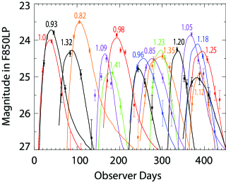
Figure 1.— Lightcurves and $z_{850}$ AB magnitudes of the high redshift SNe discovered in the survey. Each lightcurve is labeled with the SN redshift in the same color. NICMOS and $i_{775}$ observations are not shown, nor are additional SNe at $z<0.8$.

4.2. Spectroscopic Follow-up

In this paper, we describe the observations that were taken with FORS1, FORS2 and DEIMOS. The FOCAS observations are described in Morokuma et al., (2009, in preparation) and the LRIS observation of the unusual transient SN SCP06F6 is described in Barbary et al. (2009).

4.2.1 Observations with FORS1 and FORS2

With the exception of the unusual transient object SN SCP06F6 (Barbary et al., 2009), observations with FORS1 and FORS2 were performed with the 300I grism and the OG590 order sorting filter. This configuration provides a wavelength range starting at 5900 Å and extending to approximately 10000 Å with a dispersion of 2.3 Å per pixel. SN SCP06F6 was observed with the 300V grism covering a wavelength range of 3900 to 8300 Å without an order sorting filter.

Since the observations had to be carried out on short notice (we wanted the SN to be observed while it was near maximum light), most multislit observations were done with the multi-object spectroscopic (MOS) mode of FORS2 rather than with pre-cut masks. The MOS mode consists of 19 movable slits (with lengths that vary between 20” and 22”) that can be inserted into the focal plane. The slit width was set to 1”. On one occasion, we used the long slit mode on FORS1 (cluster D) and on one other occasion, when the MOS mode was unavailable on FORS2, we used a pre-cut mask (cluster C).

In observations when the SN was near maximum light, one movable slit was placed on the supernova. The other movable slits were placed on candidate cluster galaxies or field galaxies. Later, once the supernova had faded from view, a new mask was designed. Again, one movable slit was placed on the host without SN light and other movable slits were placed on candidate cluster galaxies or field galaxies. Apart from the host of the SN, we did not re-observe galaxies for which redshifts could be derived from the spectra that were obtained in the first mask.

Most clusters were observed at least twice and thus have extensive spectroscopic coverage. For each setup, between 2 and 9 exposures with exposure times varying between 600 to 900 seconds were taken. Between each exposure, the telescope was moved a few arcseconds along the slit direction. These offsets, which shift the spectra along detector columns, allow one to remove detector fringes. The process is described in Hilton et al. (2007) where additional details of data processing are found.

FORS1 and FORS2 were used to observe 14 candidates in 7 clusters. A list of the clusters that were targeted with FORS1 and FORS2 is given in Table 5. The total integration times, date of observations, and other details of the spectroscopic follow-up of clusters D, F, and R are listed in Table 6. Details for clusters A, C, U and Z are presented in Hilton et al. (2007), Santos et al. (2009), Gilbank et al. (2009, in preparation), and Rosati et al. (2009, in preparation), respectively.

Table 5 Spectroscopically targeted SNe and hosts

ID	Cluster	Instrument	SN Names
A	XMMXCS J2215.9-1738	FORS2	SN SCP06A4
C	XMMU J1229.4+0151	FORS2	SNe SCP06C0, SCP06C1, SCP06C7
D	RCS J0221.6-0347	FORS1/2	SNe SCP05D0, SCP05D6
F	ISCS J1432.4+3332	FORS2	SN SCP06F6
R	XLSS J0223.0-0436	FORS2	SN SCP06R12
U	RCS J2345.4-3632	FORS2	SNe SCP06U2, SCP06U4, SCP06U6, SCP06U7
Z	XMMU J2235.2-2557	FORS2	SNe SCP06Z5, SCP06Z13
F	ISCS J1432.4+3332	DEIMOS	SN SCP06F12
H	ISCS J1434.4+3426	DEIMOS	SN SCP06H5
K	ISCS J1438.1+3414	DEIMOS	SNe SCP06K0, SCP06K18
L	ISCS J1433.8+3325	DEIMOS	SN SCP06L21
R	XLSS J0223.0-0436	DEIMOS	SN SCP06R12
V	RCS J2319.8+0038	DEIMOS	SN SCP06V6

Table 6 Observing details for spectroscopic follow-up

ID	Instrument	Mode	Slits	Grating or Grism/Filter	Exposure times	Air Mass	Date (UT)
D	FORS1	LSS	1	300I/OG590	7x750	1.1	17/08/2005
D	FORS2	MOS	13	300I/OG590	6x900	1.1	19/12/2005
R	FORS2	MOS	12	300I/OG590	4x700	1.1	31/08/2006
R	FORS2	MOS	12	300I/OG590	6x900	1.1	30/09/2006
F	FORS2	MOS	19	300V	2x600	2.1	20/05/2006
R	DEIMOS	MOS	45	600ZD/OG550	3x1200	1.1	28/08/2006
R	DEIMOS	MOS	42	600ZD/OG550	4x1800	1.3	28/08/2006
R	DEIMOS	MOS	36	600ZD/OG550	4x1800	1.1	13/10/2007
V	DEIMOS	MOS	24	600ZD/OG550	4x1800	1.1	28/08/2006

4.2.2 Observations with DEIMOS

DEIMOS was used to observe the hosts of SN candidates in 6 clusters. A list of the clusters that were targeted with DEIMOS are given in Table 5. All observations were done using the 600ZD grating and the OG550 order sorting filter. This configuration has a typical wavelength coverage of 5000 to 10000 Å and a dispersion of 0.64 Å per pixel.

All DEIMOS observations were done with slitmasks containing between 24 and 90 slits with a width of 1”. In all masks, slits were placed on SN candidate host galaxies. Other slits were inserted on candidate cluster galaxies and field galaxies as space allowed. Spectroscopically measured redshifts for clusters F (ISCS J1432.4+3332), H (ISCS J1434.5+3427), and K (ISCS J1438.1+3414) are presented in Eisenhardt et al. (2008). Details for cluster R (XLLS J0223+0-0436), L (ISCS J1433.8+3325) and V (RCS J2319.8+0038) are presented in Table 6.

For each DEIMOS slitmask three or four exposures with exposure times varying from 1200s to 1800s were taken. We reduced the DEIMOS images with a slightly modified version of the DEEP2 pipeline developed at UC Berkeley. In total, seven SN candidates or host galaxies were observed in six clusters using the DEIMOS spectrograph.

4.2.3 Results

We obtained redshifts for all cluster SNe and all field SNe that were hosted by galaxies that were near the red-sequence at the corresponding redshift. Every SN was targeted for spectroscopic follow-up with the exception of SN SCP06Q31, SN SCP05D55, SN SCP06Z52, and SN SCP06Z53. The level of completeness in the spectroscopic follow-up allows us to rule out obvious AGN based on spectroscopic features. In total, 26 of the 35 supernovae targeted for spectroscopy have redshifts. We also obtained redshifts for over 200 cluster galaxies in a subset of 16 of the 25 clusters that were used to fill the slitmasks in parallel observations.

With the exception of SN SCP06C1, all redshifts were determined from spectroscopic features of the host galaxy. As shown in Figure 2, it was difficult to identify the host galaxy of SN SCP06C1 in the ACS images or in the follow-up spectroscopy due to contamination from a much brighter background galaxy. The well-measured spectrum of this SN (see Figure 2) clearly identifies this supernova as a SN Ia at the redshift of the cluster. SN SCP06C1 is assigned a Confidence Index of 4 for spectroscopic classification.

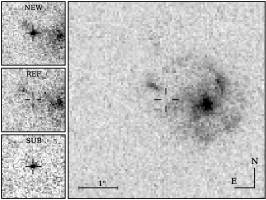
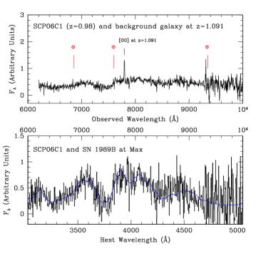
Figure 2.— Left: The panels on the left hand side demonstrate the discovery of SN SCP06C1 from the ACS images labeled ”NEW” (host galaxy with SN light), ”REF” (host only), and ”SUB” (residual after subtracting the reference image of the host galaxy). This SN occurred along the line-of-sight to a large background galaxy at $z=1.091$. The main panel shows the much brighter background galaxy centered west of the SN position and the potential SN host which lies NE of the SN position but does not have spectroscopic confirmation. Right/Upper Panel: The FORS2 spectrum of SN SCP06C1, a secure SN Ia at $z=0.98$. The [OII] $\lambda\lambda 3727$ doublet from the background galaxy can be seen in the spectrum. The spectrum is plotted in the observer frame. Strong telluric absorption features have been removed. The residuals are marked with $\oplus$. Right/Lower Panel: After subtracting the spectrum of the background galaxy, the spectrum is re-binned and plotted in the rest frame. The spectrum of SN 1989B at maximum light is the best matching nearby SN Ia. This SN is plotted at the blue continuous line.

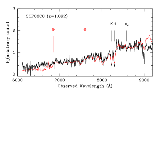
Figure 3.— The spectrum of SN SCP06C0, an example in which the SN was considerably fainter than the host galaxy (black line). The solid red line is the spectral template of an elliptical galaxy from Kinney et al. (1990). The colors of the host of SN SCP06C0 places it within the red sequence of the cluster (see Appendix A to see how this is defined) and the spectrum is, qualitatively, a good match to the spectrum of an elliptical galaxy.

The spectra of the host galaxies were generally clearly indicative of host environment. When the photometric and spectroscopic properties of the host indicated an early-type galaxy (i.e. it landed on the red sequence and the spectrum lacks obvious nebular emission lines and stellar Balmer absorption lines), then we could classify the supernova as a SN Ia with strong confidence. An example is shown in Figure 3. This typing of SNe Ia in early-type galaxies is well-established at low redshift (Cappellaro et al., 1999; Hakobyan et al., 2008). SNe that are hosted by galaxies that appear to be red-sequence galaxies are identified in a footnote in Table 3 and Table 4.

In several cases, we were able to further confirm SN type at these high-redshifts by studying the spectrum of the SN itself. Using the spectrum for supernovae that are hosted by bright early-type galaxies is a challenging task, as the hosts can be several magnitudes brighter than the supernovae. In some observations, however, we were able to observe the supernova when it was close to maximum light and when the host was not too dominant. In these cases we could identify, positively in some cases and tentatively in others, the supernova type (see Figure 2 for an example). For these SNe we followed the spectroscopic analysis procedure outlined in Lidman et al. (2005). In quite a few cases, we re-observed the host when the supernova had faded from view. By providing a measure of background contamination at the location of the SN, the second set of spectroscopic observations thus facilitates the task of subtracting the host spectrum and identifying the supernova, as shown for SNe SCP06U4 and SCP05D0 in Figure 4. With a best fit spectroscopic phase of -2 days for SN SCP05D0 and 0 days for SN SCP06U4, the spectral templates are consistent with the best fit epoch of observation from the SN lightcurves.

We quantify the degree of confidence for classification of a candidate as a SN Ia using the index described in Howell et al. (2005). A Confidence Index ranging from 5 to 0 is assigned for each SN candidate based on its spectral features and consistency with the epoch of observation predicted by the best-fit lightcurve. Candidates with 5, 4, 3, 2, 1, and 0 are certain SN Ia, highly probable SN Ia, probable SN Ia, unknown object, probably not SN Ia, and not SN Ia, respectively. We report SNe that are typed with a confidence index of 3 or higher in footnotes to Table 3 and Table 4.

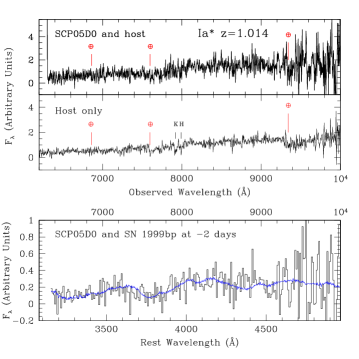
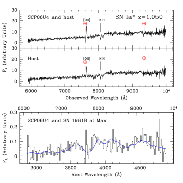
Figure 4.— Spectra of two SNe that are heavily contaminated by the light of the host galaxy. The three panels in each plot show, from top to bottom, the spectrum of the supernova and the host, the spectrum of the host without SN light, and the host-subtracted supernova spectrum in the rest frame. The best matching nearby SNe Ia are plotted in the lowest panels in blue.

SN SCP05D0 and SN SCP06U4 are both assigned a Confidence Index of 3 for spectroscopic classification, meaning that both are likely Type Ia and represented in the figure as SN Ia^∗. Not shown is the spectrum of SN SCP06D5 which was observed from VLT and classified with a Confidence Index of 3. Similarly classified SNe that were observed with Subaru will be presented in Morokuma et al. (in preparation).

4.3. SN Yield

One of the primary goals of the HST Cluster SN Survey was to increase the yield of high redshift SNe relative to previous HST surveys. With nine of the 16 SNe we identified at $z>0.95$ coming from galaxy clusters, the program demonstrates that we more than double the number of high redshift SNe by searching in rich cluster fields as shown in Figure 5. We obtain an even greater enhancement of the number of SNe in red-sequence host galaxies. Six of the nine SNe hosted by red-sequence galaxies came from clusters at $z>0.95$. These SNe offer an unbiased measure of intrinsic color and of SN properties in a specific host environment as outlined in the survey strategy.

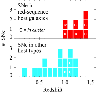
Figure 5.— The redshift distribution of the SNe discovered in our ACS program. The upper panel shows the distribution of red-sequence galaxies that had SNe Ia, with the cluster members indicated by “C”. The asterisk indicates [OII] emission in the spectrum of a galaxy with red-sequence color and spectral features as explained in the text. The lower panel shows the distribution for the other SN hosts. For $z>0.95$, the number of SNe in cluster galaxies (9) is comparable to the number of SNe in field galaxies (7).

Each SN can be checked for dust by analyzing the host properties relative to the cluster red-sequence. The host of SN SCP06U4 (Figure 4) is an interesting case. Here we observe [OII] emission in the spectrum of a galaxy with otherwise early-type color, morphology, and spectral features. There is evidence (Yan et al., 2006) that those features may be coming from quiescent red galaxies, with [OII] emission tracing AGN activity rather than star formation. After further tests of morphology, color, and spectral properties of the host of SN SCP06U4 relative to the galaxies that comprise the red-sequence of RCS234526-3632.6, this SN may yet be included in the subsample of dust-free environments.

For comparison, the SN searches in the GOODS fields were not centered on rich clusters and revealed a much lower yield of SNe hosted by early-type galaxies. In the GOODS SN program, 360 HST orbits were used in the initial search and more than 390 additional orbits were used to obtain full lightcurves and spectral confirmation of 23 SNe at $z>1$. Six SNe with early-type hosts were discovered at $z>0.9$ (Riess et al., 2007). Scaling the yield of SNe from our 219-orbit program, we would expect to find 27 red-sequence hosted SNe with complete lightcurves in the same total number of orbits as the GOODS program in the same redshift range. If we only consider the ACS search visits for the two programs (360 vs 188), we would expect to discover 15 red-sequence hosted SNe with complete lightcurves in fields with rich clusters as opposed to the six that were discovered in the GOODS survey. In the following section we will discuss the boost in SNe from an astrophysical perspective, here we explain the additional gain due to the efficiency of the survey strategy.

There are several reasons for the improved efficiency from this new observation technique. For one, the density enhancement of galaxies in the cluster fields provides more potential $z>0.9$ SN hosts than in a blind search. This increases the percentage of orbits in the pre-scheduled observations with active SN light - 67 of the 188 ACS orbits were effectively used to measure SNe lightcurves in clusters compared to 54 orbits for SNe hosted by $z>0.95$ field galaxies. The shorter amount of time between observations of a given cluster field also increases the likelihood that a SN is discovered early in its lightcurve. Early discovery enables the scheduling of a single high signal-to-noise NICMOS observation near maximum light for constraints on color for SNe at $z<1.3$ and a full lightcurve of NICMOS observations for SNe at higher redshift. Finally, the SNe can be characterized by the evolutionary history of their red-sequence host galaxies. SNe Ia can therefore be identified with similar confidence to high redshift SNe from previous programs without difficult direct spectroscopic typing.

5. Discussion: SN Production in Clusters

The results obtained with this SN survey show qualitative and quantitative improvements in the SN yield per orbit over a SN survey targeting random fields. It is also important to determine if they are consistent with the improvement expected from the overdensity of red-sequence galaxies in the targeted clusters. Here we compare the distribution of cluster SNe and the increased discovery rate to the distribution and overdensity of red-sequence cluster members.

Figure 6.— Red-sequence of WARP J1415.1+3612 compared to field galaxies from the GOODS data. (a) Left: The color magnitude diagram for galaxies in the image of WARP J1415.1+3612. (b) Center: The color magnitude-diagram for galaxies in a random GOODS field of the same area. In both color magnitude diagrams, the solid circles represent galaxies with a color and morphology expected for an early type cluster member, the open circles represent all galaxies in the image, and the solid line illustrates the modeled red-sequence at $z=1.03$. Some objects represented by open circles had colors and magnitudes near the red-sequence but did not have morphologies consistent with an elliptical galaxy. Other objects had a morphology consistent an elliptical galaxy but did not lie near the model red-sequence. (c) Right: Histogram of the red-sequence members and interlopers. The solid line represents galaxies within 0.1 mag of the red-sequence in WARP J1415.1+3612 and the dashed line represents an estimate of interlopers derived from the GOODS fields.

We compute a measure of the red-sequence richness, $N_{red}$, following the approach outlined in Appendix A. The parameter $N_{red}$ serves as a proxy for the total stellar mass in cluster-elliptical galaxies, and thus provides the relative density comparisons. In another analysis (Barbary et al., in prep) we address the more detailed questions required to compare SN production at high and low redshifts, and place constraints on the evolution of delay times for SNe Ia in early-type cluster galaxies. This further analysis will include the precise determination of total cluster luminosity, SN detection efficiency, and the window of time probed during the survey.

The red-sequence richnesses and $68\%$ uncertainties are found in Table 3. As an example of the method, we show the results for the $z=1.03$ cluster WARP J1415.1+3612 (cluster “E” in Table 3) in Figure 6. The red-sequence galaxies appear as a clear overdensity for this cluster relative to the HST GOODS (Giavalisco et al., 2004) fields.

The mean red-sequence richness of this sample of clusters computed within a 1 Mpc radius field of view is $N_{red}=15.9$. This average red-sequence richness is a factor of 1.2 higher than the number of field galaxies that would be identified as $0.9<z<1.5$ red-sequence galaxies in an arbitrary ACS observation. We therefore expect roughly 1.2 SNe hosted by cluster red-sequence galaxies for every SN hosted by a random $z>0.9$ red-sequence galaxy, or 2.2 times as many red-sequence hosted SNe in this HST program compared to an HST survey of random fields.

The $N_{red}$ parameter serves as a proxy for cluster richness. For comparison, we computed the total luminosity of the cluster red-sequence galaxies relative to the field galaxies using MAG_AUTO (Bertin & Arnouts, 1996) as a first order estimate of total light. The overdensity in cluster luminosity relative to the field was found to be more significant than the overdensity represented by the $N_{red}$ parameter, indicating that the $N_{red}$ parameter underestimates the cluster luminosity. Considering that the average cluster red-sequence galaxy in this sample is brighter than the average interloper, and given the fluctuations expected from Poisson statistics, the ratio of six cluster red-sequence SNe to three field red-sequence SNe discovered in the program may be consistent with the increase that would be expected. It is also possible that the increase is due to a true enchancement of the SN Ia rate in cluster red-sequence galaxies relative to field red-sequence galaxies, as recently found at low redshift by Mannucci et al. (2008). A more detailed determination of SN yield with cluster luminosity will be reported in the aforementioned analysis of SN rates in galaxy clusters.

The radial distribution of SNe discovered in clusters is shown in Table 3. Although only $27.7\%$ of the ACS field of view lies within $1^{\prime}$ of the cluster center, eight of the nine cluster hosted SNe were found inside this radius. The high density of SN events near the cluster core traces the distribution of red-sequence galaxies as shown in Figure 7.

Applying a Kolmogorov-Smirnov (K-S) statistic analysis to the cumulative distribution yields a maximum separation $D=0.251$. The probability of obtaining this separation or larger in a sample of nine SNe is approximately $55\%$, demonstrating consistency between the two distributions. Examination of the increase in yield and distribution of SNe therefore leads us to conclude that the strategy of targeting galaxy clusters improved the survey efficiency with HST as expected.

A further dramatic result is shown in Figure 8 - the richer clusters were primarily responsible for the increased productivity. The median red-sequence richness of clusters producing a SN was $N_{red}=20.4$ while the median for clusters not producing a SN was $N_{red}=12.1$.

Figure 7.— (a) Upper Panel: Cumulative distribution of red-sequence galaxies in all 25 clusters with 21 $<z_{850}<$ 24 selected (solid line) and SNe (dashed line and solid circles). (b) Lower Panel: The solid line represents the surface density as a function of distance from the cluster center of galaxies with 21 $<z_{850}<$ 24 selected to lie on the red-sequence for the complete sample of 25 clusters in this program. The dashed line represents the surface density of galaxies satisfying the same criteria in the GOODS data. The histogram represents the surface density of cluster SNe from this program. Because some of the cluster volume may lie outside the field, surface densities are computed from the number of pixels in the stacked ACS images within a distance $r$ from the cluster center.

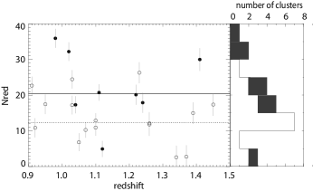
Figure 8.— Red-sequence richness as a function of redshift. Clusters that hosted supernovae are indicated with filled symbols. Clusters that did not host supernova are indicated with open symbols. The solid and dotted lines mark the respective median richnesses of the two samples. The histogram represents the distribution of richnesses for clusters that did not host a SN (open) and for clusters that did (filled).

6. Conclusion

The strategy of targeting high redshift galaxy clusters results in a significant boost in the yield of high redshift SNe. The increased yield from cluster SNe is consistent with expectations from the overdensity of red-sequence galaxies. Nine of the 16 SNe at $z>0.95$ were discovered in galaxy clusters and six of the nine SNe hosted by red-sequence galaxies were discovered in the cluster environment. By doubling the number of total SNe and tripling the number of SNe hosted by red-sequence galaxies, the new technique of targeting massive clusters with HST has met its first measurable goal.

The cosmological analysis will be presented in a separate paper with SN lightcurves and a new high redshift Hubble diagram. The new sample will be large enough to be used together with a similar sample of low and moderate redshift SNe to begin to study the implications of host galaxy environment with respect to SN properties and derived cosmology. In addition, the SNe in this survey will provide improved constraints on SN production in high redshift clusters compared to previous studies (Gal-Yam et al., 2002; Sharon et al., 2007; Mannucci et al., 2008; Graham et al., 2008). Finally, these deep ACS images also enable key studies of the evolution of massive galaxies and clusters, the measurement of cluster masses via weak lensing, and an entire program of cluster studies. Several related parallel analyses have already been submitted or published (Melbourne et al., 2007; Hilton et al., 2007; Eisenhardt et al., 2008; Barbary et al., 2009; Hilton et al., 2009; Santos et al., 2009) using data from this program.

The results of this program are very promising for SN surveys using the next generation of HST instruments like the IR channel of WFC3. The WFC3 IR field of view is $60\%$ smaller than ACS but still would have captured eight of the nine of the cluster SNe discovered in the ACS program. A SN survey targeting the same sample of galaxy clusters with WFC3 would thus be expected to produce nearly the same yield of cluster hosted SNe. On the other hand, a conventional SN survey that does not target clusters would suffer a drop in yield proportional to the loss of survey area. More massive clusters at redshifts out to nearly $z=1.4$ have been discovered in recent surveys that were not available when the HST Cluster SN Survey took place (e.g. Eisenhardt et al., 2008; Wilson et al., 2009; Muzzin et al., 2009). Since almost all cluster SNe were found in the richest of the clusters targeted with ACS, a future survey targeting these newly discovered rich clusters would lead to an even further increase in the rate of SNe per orbit. A WFC3 survey would also provide better sensitivity in the NIR, stretching SN studies to higher redshifts with even better signal-to-noise than was achieved with ACS. Such a program would yield a SN in every cluster, bringing the technique to its logical conclusion as every HST observation would be used to constrain the SN lightcurve in a pre-scheduled search with no additional follow-up imaging.

We thank Julien Guy, Pierre Astier, and Josh Frieman for stimulating discussion of SN color and host type from their experience in the analyses of the large SNLS and SDSS-II SN data sets. We thank the Aspen Center for Physics for its summer 2007 hospitality during the preparation of this paper. Financial support for this work was provided by NASA through program GO-10496 from the Space Telescope Science Institute, which is operated by AURA, Inc., under NASA contract NAS 5-26555. This work was also supported in part by the Director, Office of Science, Office of High Energy and Nuclear Physics, of the U.S. Department of Energy under Contract No. AC02-05CH11231, as well as a JSPS core-to-core program “International Research Network for Dark Energy” and by JSPS research grant 20040003. Support for MB was provided by the W. M. Keck Foundation. The work of SAS was performed under the auspices of the U.S. Department of Energy by Lawrence Livermore National Laboratory in part under Contract W-7405-Eng-48 and in part under Contract DE-AC52-07NA27344. The work of PE, JR, and DS was carried out at the Jet Propulsion Laboratory, California Institute of Technology, under a contract with NASA.

Subaru observations were collected at Subaru Telescope, which is operated by the National Astronomical Observatory of Japan. Some of the data presented herein were obtained at the W.M. Keck Observatory, which is operated as a scientific partnership among the California Institute of Technology, the University of California, and the National Aeronautics and Space Administration. The authors wish to recognize and acknowledge the very significant cultural role and reverence that the summit of Mauna Kea has always had within the indigenous Hawaiian community. We are most fortunate to have the opportunity to conduct observations from this mountain. Some of spectroscopic data presented in this paper were taken at the Cerro Paranal Observatory as part of ESO programs 171.A-0486, 276.A-5034, 077.A-0110 and 078.A-0060.

Appendix A Computing the Red-Sequence Richness

To compute the red-sequence richness of clusters, we used spectroscopically confirmed early-type galaxies from the observations discussed briefly in §4.2 to model the red-sequence. We identified the subsample of early-type galaxies with no significant [OII] emission and a redshift determined from the Ca II H & K absorption lines. In total, 64 early-type galaxies from these observations were used to develop an empirical model for the red-sequence for the sample of 25 clusters at these high redshifts.

We used only the photometry from the deep $i_{775}$ and $z_{850}$ ACS images to generate a model for the red-sequence. The photometry was performed using the SExtractor (Bertin & Arnouts, 1996) analysis package. The analysis of 19 early-type galaxies from RDCS J1252.9-2927 (Demarco et al., 2007) and 14 from XMMU J1229.4+0151 produced an observed RMS scatter from the empirically derived red-sequence of $0.043$ mag and $0.048$ magnitudes respectively. The photometry here was developed to classify potential red-sequence SN hosts and was not optimized to measure the intrinsic dispersion, resulting in a slightly larger RMS scatter in RDCS J1252.9-2927 than reported in Blakeslee et al. (2003).

Assuming a 2.5 Gyr stellar population, simple stellar populations of varying metallicity were used to generate synthetic elliptical galaxy templates (Bruzual & Charlot, 2003) for the K-corrections. For each galaxy, we chose a template with metallicity that produced the observed $i_{775}$-$z_{850}$ color and scaled that template to match the observed $z_{850}$ magnitude. These spectral templates were redshifted and passed through the ACS response curves (Mack et al., 2007) to generate synthetic $i_{775}$ and $z_{850}$ photometry for each cluster. The synthetic $i_{775}$ and $z_{850}$ photometry was used to populate a color magnitude diagram for each cluster after correcting for luminosity distance.

Photometric catalogs were generated with the same SExtractor parameters applied to all objects in the cluster fields that were used to obtain the photometry of the 64 galaxies that modeled the red-sequence. Objects with stellar or disk-like morphologies identified by CLASS_STAR $>\,0.7$, ELLIPTICITY $>\,0.5$, or FWHM_IMAGE $<\,3.5$ pixels were excluded. For each ACS field, the remaining galaxies in the catalog were compared to the model red-sequence at the redshift of the target cluster. All galaxies with a $i_{775}$-$z_{850}$ color within 0.1 mag of the model red sequence were identified as likely elliptical cluster members. This criteria was also used to identify SN hosts as “red-sequence” galaxies. The red-sequence at the host redshift was used as the template for cluster and non-cluster SNe.

Many galaxy clusters host a bright cD galaxy that is often used to define the cluster center. However, several clusters in this sample have two bright central galaxies or no clear cD galaxy at all. We therefore introduce a simple algorithm to define the center of a cluster. First, we computed a rough centroid determined by the average position of all galaxies with color and luminosity consistent with the model red-sequence. Next, we selected the five brightest galaxies within 0.3 - 0.6 Mpc of the rough center, where the exact aperture depended on the number of red-sequence galaxies and compactness of the cluster. The final center was chosen to minimize the square of the differences to these five galaxies.

To estimate the number of field galaxies that appear as interlopers in the red-sequence, we performed an identical analysis using the $i_{775}$ and $z_{850}$ images from the north and south HST GOODS survey. The GOODS images were processed using MultiDrizzle with the same output pixel scale as the cluster fields. The GOODS fields were observed in two different orientations distinguished by a 45 degree relative rotation. These observations roughly reproduce any PSF artifacts that may be induced by the variety of telescope roll angles in the observations of the cluster fields. Objects in the GOODS fields that pass the selection tests described above were used to represent the population of interloper field galaxies that would be expected to appear in any ACS pointing.

The red-sequence richness, $N_{red}$, was determined from the number of red-sequence galaxies inside an aperture on the cluster center. As shown in Figure 7, the surface density of interlopers is approximately equal to the surface density of cluster galaxies at a distance $0.6$ Mpc from the cluster center. More than $80\%$ of the galaxies in the composite cluster are contained in a 0.6 Mpc radius aperture. Essentially all red-sequence cluster members are included inside a radius of 1.0 Mpc. This aperture size is also fairly well matched to the ACS field of view and was chosen to estimate the red-sequence richnesses.

We sought a measure of the red-sequence richness that avoids the Poisson noise from having very few members at the bright end of the luminosity function. At the same time, we tried to provide a measure that represents the clusters at all redshifts without substantial measurement error. To do so, we anchored the measurement at a magnitude $M^{\prime}$ near the faint end of the red sequence assuming linear passive evolution with $dM/dz=-1$ in the rest frame luminosity. $M^{\prime}$ was chosen to be near the background dominated limit for the most distant clusters in the sample, $M^{\prime}=24.5$ in the $z_{850}$ filter at $z=1.5$. For comparison, in a model assuming passive evolution, $z_{850}=23.61$ for $L_{*}$ at $z=1.5$. The red-sequence richness was then defined as the number of red-sequence galaxies inside a 1 Mpc aperture with $M^{\prime}-2<z_{850}<M^{\prime}$. Interloper field galaxies at other redshifts were removed by subtracting the number of GOODS galaxies satisfying the same cut in the same survey area. Uncertainties in the background subtraction were estimated from the Poisson statistics of the GOODS catalogs. The uncertainty in the photometric redshifts of ISCS J1433.8+3325 and RCS033750-2844.8 could impact the measurements of $N_{red}$. To test for additional systematic errors, $N_{red}$ was computed for these two clusters at a redshift of $z=z_{phot}\pm 0.1$. The measurements did not indicate any significant deviation from the uncertainties estimated from the GOODS catalogs.

References

- Aldering et al. (2002) Aldering, G., et al. 2002, in Survey and Other Telescope Technologies and Discoveries, Proceedings of the SPIE, ed. J. A. Tyson & S. Wolff, Vol. 4836, 61–72
- Aldering et al. (1998) Aldering, G., et al. 1998, IAU Circ., 7046, 1
- Andreon et al. (2005) Andreon, S., Valtchanov, I., Jones, L. R., Altieri, B., Bremer, M., Willis, J., Pierre, M., & Quintana, H. 2005, MNRAS, 359, 1250
- Appenzeller et al. (1998) Appenzeller, I., et al. 1998, The Messenger, 94, 1
- Astier et al. (2006) Astier, P., et al. 2006, A&A, 447, 31
- Barbary et al. (2009) Barbary, K., et al. 2009, ApJ, 690, 1358
- Bertin & Arnouts (1996) Bertin, E. & Arnouts, S. 1996, A&AS, 117, 393
- Blakeslee et al. (2003) Blakeslee, J. P., et al. 2003, ApJ, 596, L143
- Bohringer et al. (2005) Bohringer, H., Mullis, C., Rosati, P., Lamer, G., Fassbender, R., Schwope, A., & Schuecker, P. 2005, The Messenger, 120, 33
- Bower et al. (1992) Bower, R. G., Lucey, J. R., & Ellis, R. S. 1992, MNRAS, 254, 601
- Bremer et al. (2006) Bremer, M. N., et al. 2006, MNRAS, 371, 1427
- Brodwin et al. (2006) Brodwin, M., et al. 2006, ApJ, 651, 791
- Bruzual & Charlot (2003) Bruzual, G. & Charlot, S. 2003, MNRAS, 344, 1000
- Cain et al. (2008) Cain, B., et al. 2008, ApJ, 679, 293
- Cappellaro et al. (1999) Cappellaro, E., Evans, R., & Turatto, M. 1999, A&A, 351, 459
- Chelouche et al. (2007) Chelouche, D., Koester, B. P., & Bowen, D. V. 2007, ApJ, 671, L97
- Coil et al. (2000) Coil, A. L., et al. 2000, ApJ, 544, L111
- Conley et al. (2007) Conley, A., Carlberg, R. G., Guy, J., Howell, D. A., Jha, S., Riess, A. G., & Sullivan, M. 2007, ApJ, 664, L13
- Demarco et al. (2007) Demarco, R., et al. 2007, ApJ, 663, 164
- Dunkley et al. (2009) Dunkley, J., et al. 2009, ApJS, 180, 306
- Eisenhardt et al. (2008) Eisenhardt, P. R. M., et al. 2008, ApJ, 684, 905
- Eisenstein et al. (2005) Eisenstein, D. J., et al. 2005, ApJ, 633, 560
- Ellis et al. (1997) Ellis, R. S., Smail, I., Dressler, A., Couch, W. J., Oemler, A. J., Butcher, H., & Sharples, R. M. 1997, ApJ, 483, 582
- Elston et al. (2006) Elston, R. J., et al. 2006, ApJ, 639, 816
- Faber et al. (2003) Faber, S. M., et al. 2003, in Society of Photo-Optical Instrumentation Engineers (SPIE) Conference Series, ed. M. Iye & A. F. M. Moorwood, Vol. 4841, 1657–1669
- Filippenko et al. (2001) Filippenko, A. V., Li, W. D., Treffers, R. R., & Modjaz, M. 2001, in Astronomical Society of the Pacific Conference Series, Vol. 246, IAU Colloq. 183: Small Telescope Astronomy on Global Scales, ed. B. Paczynski, W.-P. Chen, & C. Lemme, 121
- Frieman et al. (2008) Frieman, J. A., et al. 2008, AJ, 135, 338
- Fruchter & Hook (2002) Fruchter, A. S. & Hook, R. N. 2002, PASP, 114, 144
- Gal-Yam et al. (2002) Gal-Yam, A., Maoz, D., & Sharon, K. 2002, MNRAS, 332, 37
- Garnavich et al. (1998) Garnavich, P. M., et al. 1998, ApJ, 509, 74
- Giavalisco et al. (2004) Giavalisco, M., et al. 2004, ApJ, 600, L93
- Gilbank et al. (2008) Gilbank, D. G., Yee, H. K. C., Ellingson, E., Hicks, A. K., Gladders, M. D., Barrientos, L. F., & Keeney, B. 2008, ApJ, 677, L89
- Gladders & Yee (2005) Gladders, M. D. & Yee, H. K. C. 2005, ApJS, 157, 1
- Goobar (2008) Goobar, A. 2008, ApJ, 686, L103
- Graham et al. (2008) Graham, M. L., et al. 2008, AJ, 135, 1343
- Guy et al. (2005) Guy, J., Astier, P., Nobili, S., Regnault, N., & Pain, R. 2005, A&A, 443, 781
- Hakobyan et al. (2008) Hakobyan, A. A., Petrosian, A. R., McLean, B., Kunth, D., Allen, R. J., Turatto, M., & Barbon, R. 2008, A&A, 488, 523
- Hamuy et al. (2006) Hamuy, M., et al. 2006, PASP, 118, 2
- Hamuy et al. (2000) Hamuy, M., Trager, S. C., Pinto, P. A., Phillips, M. M., Schommer, R. A., Ivanov, V., & Suntzeff, N. B. 2000, AJ, 120, 1479
- Hicken et al. (2009) Hicken, M., Wood-Vasey, W. M., Blondin, S., Challis, P., Jha, S., Kelly, P. L., Rest, A., & Kirshner, R. P. 2009, ArXiv e-prints
- Hicks et al. (2008) Hicks, A. K., et al. 2008, ApJ, 680, 1022
- Hilton et al. (2007) Hilton, M., et al. 2007, ApJ, 670, 1000
- Hilton et al. (2009) Hilton, M., et al. 2009, ApJ, 697, 436
- Hogg et al. (2004) Hogg, D. W., et al. 2004, ApJ, 601, L29
- Howell et al. (2005) Howell, D. A., et al. 2005, ApJ, 634, 1190
- Jha et al. (2007) Jha, S., Riess, A. G., & Kirshner, R. P. 2007, ApJ, 659, 122
- Kashikawa et al. (2002) Kashikawa, N., et al. 2002, PASJ, 54, 819
- Kinney et al. (1990) Kinney, A. L., Rivolo, A. R., & Koratkar, A. P. 1990, ApJ, 357, 338
- Koekemoer et al. (2002) Koekemoer, A. M., Fruchter, A. S., Hook, R. N., & Hack, W. 2002, in The 2002 HST Calibration Workshop : Hubble after the Installation of the ACS and the NICMOS Cooling System, ed. S. Arribas, A. Koekemoer, & B. Whitmore, 337
- Kowalski et al. (2008) Kowalski, M., et al. 2008, ApJ, 686, 749
- Kuznetsova et al. (2008) Kuznetsova, N., et al. 2008, ApJ, 673, 981
- Lidman et al. (2005) Lidman, C., et al. 2005, A&A, 430, 843
- Lidman et al. (2008) Lidman, C., et al. 2008, A&A, 489, 981
- Mack et al. (2007) Mack, J., Gilliland, R. L., Anderson, J., & Sirianni, M. 2007, WFC Zeropoints at -80C, Instrument Science Report ACS 2007-02, Tech. rep.
- Mannucci et al. (2005) Mannucci, F., Della Valle, M., Panagia, N., Cappellaro, E., Cresci, G., Maiolino, R., Petrosian, A., & Turatto, M. 2005, A&A, 433, 807
- Mannucci et al. (2008) Mannucci, F., Maoz, D., Sharon, K., Botticella, M. T., Della Valle, M., Gal-Yam, A., & Panagia, N. 2008, MNRAS, 383, 1121
- Mei et al. (2006a) Mei, S., et al. 2006a, ApJ, 639, 81
- Mei et al. (2009) Mei, S., et al. 2009, ApJ, 690, 42
- Mei et al. (2006b) Mei, S., et al. 2006b, ApJ, 644, 759
- Melbourne et al. (2007) Melbourne, J., et al. 2007, AJ, 133, 2709
- Mullis et al. (2005) Mullis, C. R., Rosati, P., Lamer, G., Böhringer, H., Schwope, A., Schuecker, P., & Fassbender, R. 2005, ApJ, 623, L85
- Muzzin et al. (2009) Muzzin, A., et al. 2009, ApJ, 698, 1934
- Nobili & Goobar (2008) Nobili, S. & Goobar, A. 2008, A&A, 487, 19
- Oke et al. (1995) Oke, J. B., et al. 1995, PASP, 107, 375
- Perlman et al. (2002) Perlman, E. S., Horner, D. J., Jones, L. R., Scharf, C. A., Ebeling, H., Wegner, G., & Malkan, M. 2002, ApJS, 140, 265
- Perlmutter et al. (1998) Perlmutter, S., et al. 1998, Nature, 391, 51
- Perlmutter et al. (1999) Perlmutter, S., et al. 1999, ApJ, 517, 565
- Perlmutter et al. (1997) Perlmutter, S., et al. 1997, ApJ, 483, 565
- Perlmutter et al. (1995) Perlmutter, S., et al. 1995, ApJ, 440, L41
- Perlmutter & Schmidt (2003) Perlmutter, S. & Schmidt, B. P. 2003, in Lecture Notes in Physics, Berlin Springer Verlag, Vol. 598, Supernovae and Gamma-Ray Bursters, ed. K. Weiler, 195–217
- Phillips (1993) Phillips, M. M. 1993, ApJ, 413, L105
- Phillips et al. (1999) Phillips, M. M., Lira, P., Suntzeff, N. B., Schommer, R. A., Hamuy, M., & Maza, J. 1999, AJ, 118, 1766
- Postman et al. (1996) Postman, M., Lubin, L. M., Gunn, J. E., Oke, J. B., Hoessel, J. G., Schneider, D. P., & Christensen, J. A. 1996, AJ, 111, 615
- Postman et al. (2001) Postman, M., Lubin, L. M., & Oke, J. B. 2001, AJ, 122, 1125
- Reiss et al. (1998) Reiss, D. J., Germany, L. M., Schmidt, B. P., & Stubbs, C. W. 1998, AJ, 115, 26
- Riess et al. (1998) Riess, A. G., et al. 1998, AJ, 116, 1009
- Riess et al. (1995) Riess, A. G., Press, W. H., & Kirshner, R. P. 1995, ApJ, 438, L17
- Riess et al. (1996) —. 1996, ApJ, 473, 88
- Riess et al. (2007) Riess, A. G., et al. 2007, ApJ, 659, 98
- Rosati et al. (1999) Rosati, P., Stanford, S. A., Eisenhardt, P. R., Elston, R., Spinrad, H., Stern, D., & Dey, A. 1999, AJ, 118, 76
- Rosati et al. (2004) Rosati, P., et al. 2004, AJ, 127, 230
- Sahlen et al. (2008) Sahlen, M., et al. 2008, ArXiv e-prints
- Santos et al. (2009) Santos, J. S., et al. 2009, ArXiv e-prints
- Schmidt et al. (1998) Schmidt, B. P., et al. 1998, ApJ, 507, 46
- Sharon et al. (2007) Sharon, K., Gal-Yam, A., Maoz, D., Filippenko, A. V., & Guhathakurta, P. 2007, ApJ, 660, 1165
- Stanford et al. (2005) Stanford, S. A., et al. 2005, ApJ, 634, L129
- Stanford et al. (1998) Stanford, S. A., Eisenhardt, P. R., & Dickinson, M. 1998, ApJ, 492, 461
- Stanford et al. (2002) Stanford, S. A., Holden, B., Rosati, P., Eisenhardt, P. R., Stern, D., Squires, G., & Spinrad, H. 2002, AJ, 123, 619
- Stanford et al. (2006) Stanford, S. A., et al. 2006, ApJ, 646, L13
- Sullivan et al. (2003) Sullivan, M., et al. 2003, MNRAS, 340, 1057
- Sullivan et al. (2006) Sullivan, M., et al. 2006, ApJ, 648, 868
- Takanashi et al. (2008) Takanashi, N., Doi, M., & Yasuda, N. 2008, MNRAS, 389, 1577
- Temi et al. (2005) Temi, P., Brighenti, F., & Mathews, W. G. 2005, ApJ, 635, L25
- Tonry et al. (1999) Tonry, J., et al. 1999, IAU Circ., 7312, 1
- Tran et al. (2001) Tran, H. D., Tsvetanov, Z., Ford, H. C., Davies, J., Jaffe, W., van den Bosch, F. C., & Rest, A. 2001, AJ, 121, 2928
- Tripp (1998) Tripp, R. 1998, A&A, 331, 815
- Wilson et al. (2009) Wilson, G., et al. 2009, ApJ, 698, 1943
- Wood-Vasey et al. (2007) Wood-Vasey, W. M., et al. 2007, ApJ, 666, 694
- Yan et al. (2006) Yan, R., Newman, J. A., Faber, S. M., Konidaris, N., Koo, D., & Davis, M. 2006, ApJ, 648, 281
- Yee et al. (2007) Yee, H. K. C., Gladders, M. D., Gilbank, D. G., Majumdar, S., Hoekstra, H., & Ellingson, E. 2007, in Astronomical Society of the Pacific Conference Series, Vol. 379, Cosmic Frontiers, ed. N. Metcalfe & T. Shanks, 103