Asymptotics of conduction velocity restitution in models of electrical excitation in the heart
Abstract
We extend a non-Tikhonov asymptotic embedding, proposed earlier, for calculation of conduction velocity restitution curves in ionic models of cardiac excitability. Conduction velocity restitution is the simplest nontrivial spatially extended problem in excitable media, and in the case of cardiac tissue it is an important tool for prediction of cardiac arrhythmias and fibrillation. An idealized conduction velocity restitution curve requires solving a nonlinear eigenvalue problem with periodic boundary conditions, which in the cardiac case is very stiff and calls for the use of asymptotic methods. We compare asymptotics of restitution curves in four examples, two generic excitable media models, and two ionic cardiac models. The generic models include the classical FitzHugh-Nagumo model and its variation by Barkley. They are treated with standard singular perturbation techniques. The ionic models include a simplified “caricature” of the Noble (1962) model and the Beeler and Reuter (1977) model, which lead to non-Tikhonov problems where known asymptotic results do not apply. The Caricature Noble model is considered with particular care to demonstrate the well-posedness of the corresponding boundary-value problem. The developed method for calculation of conduction velocity restitution is then applied to the Beeler-Reuter model. We discuss new mathematical features appearing in cardiac ionic models and possible applications of the developed method.
1 Department of Mathematics, University of Glasgow, Glasgow G12 8QW, UK
2 Department of Mathematical Sciences, University of Liverpool, Liverpool L69 7ZL, UK
Keywords action potential; traveling wave.
1 Introduction
Cardiac excitability models
Hodgkin and Huxley’s model of the electric properties of the giant squid axon [30] was the first to describe in mathematical terms the exclusively biological phenomenon of excitability. It started a revolution in science well-worth the Nobel prize it was awarded. This achievement has been followed by the development of a long sequence of mathematical models of heart excitability starting from Noble’s works [49, 50]. Due to its importance for biomedical applications, particularly for understanding and treatment of cardiac arrhythmias caused by pathologies of electrical excitation and propagation, the mathematical modelling direction has been under intensive development during the last decades, and currently has reached clinical applications and industrial scale. It lies in the heart of the ambitious Physiome project [31] which aims at a mathematical description of the physiology of whole organisms. Due to complexity of the models involved they are mainly used in numerical computations and contribute a substantial load on the UK national supercomputer facilities [52].
Stiffness of cardiac excitability models
The computational complexity of cardiac models lies not only in the complexity of the heart as a system, which compared to the brain is relatively modest, but also in the essential stiffness of cardiac equations. These equations have to describe very sharp and fast excitation fronts where some processes happen on the scale of tens of microseconds and micrometers, through to tissue and organ level, on the scale of seconds and centimeters, thus covering several orders of magnitude. Thus a challenge for applied mathematics is how to turn this stiffness from an adversary into an ally. A standard approach is to treat small parameters, responsible for such stiffness, using asymptotic rather than numerical methods. For the Hodgkin-Huxley model, a simple caricature easily treatable mathematically has been introduced by FitzHugh [23] and Nagumo et al. [48], which was based on a modification of the classical van der Pol system of equations [60]. Asymptotic analysis of FitzHugh-Nagumo type systems, a nice summary of which can be found e.g. in [59], has achieved remarkable success in describing, in qualitative terms, many of the phenomena observed in more realistic, experiment based ionic models.
The traditional asymptotic approach
The essence of the approach is separation of the dynamic variables into “fast and slow”, similar to the classical Tikhonov-Pontryagin scheme [58, 53, 45], only in a spatially extended context. A typical solution consists of moving, fast and steep “fronts” and “backs” of excitation pulses, located near codimension-one manifolds, i.e. points in one spatial dimension (1D), lines in two spatial dimensions (2D), and surfaces in three spatial dimensions (3D), which are interspersed by smooth and slow intervals. During the fast fronts and backs, the slow variables remain almost unchanged. During the slow intervals, the fast variables remain very close to their quasi-stationary values determined by the current values of the slow variables. The slow pieces are typically of two kinds: with lower and with higher values of the transmembrane voltage or a variable that corresponds to it. The lower-voltage, “diastolic” pieces are close to or include the “resting state”, representing excitable tissue which was not excited for a long time, and the higher-voltage, “systolic” pieces represent the “action potential” phase of the excitation. An extra feature of 2D and 3D is the possibility of “wave breaks”, which are of particular relevance for cardiac arrhythmias. Such wave breaks are moving codimension-two manifolds, i.e. points in 2D and lines in 3D, where the fronts and backs meet. It is essential that mathematically, fronts and backs are objects of the same nature, differing only in the direction of motion: at the fronts, the systolic phase advances; at the backs, the systolic phase recedes, so the wave break is where the interface between the phases is momentarily stalled. This description allows even some analytical treatment of the motion of wave breaks in 2D, including steadily rotating and meandering spiral waves of excitation [26]. Conceivably, this asymptotic description could be also used numerically within an appropriate moving interface methodology.
The need for a non-Tikhonov embedding
However, since models of FitzHugh-Nagumo type have been typically postulated rather than derived from realistic ionic models of cardiac excitation, the question about their quantitative validity was not usually posed. Successful attempts to apply the same singular perturbation technique as developed for systems of FitzHugh-Nagumo type, directly to detailed ionic models, have been made, e.g. [39], but this did not turn into a mainstream practical approach. We believe that the reason is that systems of FitzHugh-Nagumo type are actually quite different, in the asymptotic sense, from detailed ionic cardiac models, as they fail completely to describe, even at a qualitative level, some important properties of cardiac excitation, such as
-
•
slow reporarization,
-
•
slow subthreshold response,
-
•
fast accommodation,
-
•
variable peak voltage and
-
•
front dissipation,
all of which are experimentally well-established and also successfully reproduced by detailed cardiac ionic models [8, 10]. The slow repolarization means that, although cardiac excitation pulses do indeed possess steep fronts, they have no steep backs, at least not steep enough compared to the steepness of the fronts, anyway. Hence interpretation of wave breaks in 2D and 3D as loci where fronts meet backs is inapplicable to cardiac models for absence of backs. Since propagation blocks and wave breaks are very important in most applications of mathematical cardiology, there is no much hope that the FitzHugh-Nagumo ideology could lead to a practical numerical tool that could tame the stiffness of the cardiac equations.
In a recent series of works [8, 9, 12, 10], we have developed an analytical approach to cardiac equations based on their special structure, different from the FitzHugh-Nagumo paradigm, and taking into account small parameters actually present (sometimes hidden) in the equations, rather than trying to force them into the Procrustean bed of a classical scheme. Using the existence of large (or small) values of some variables for model reduction and perturbation analysis is a basic technique in applied mathematics. One well-known example is the Quasi(Pseudo)-Steady-State approximation [27, 55], which reduces the equations of an enzyme reaction to a singular perturbation Tikhonov problem. Another prominent example is the wide application of scale separation and model reduction techniques to problems of chemical kinetics and reactive flows. Since in such problems the number of reacting species is huge, this is typically done by computational algorithms such as Computational Singular Perturbations (CSP), Intrinsic Low-Dimensional Manifolds (ILDM), the Grad Moment method and others [25, 34]. It has been shown that these computational techniques generate the asymptotic expansion of a slow invariant manifold of a Tikhonov problem [34, 64].
However, the application of asymptotic embedding techniques is not restricted to Tikhonov problems, nor must it, a priori, lead to such. Indeed, our recent works [8, 9, 12, 10] have clearly demonstrated that, to achieve a physiologically correct asymptotics in realistic models of cardiac excitation, a parameter embedding is needed which involves a large factor in front of individual terms, but not the whole, of the right-hand side of some equations (e.g. the term in the transmembrane voltage evolution equation), non-analytical, perhaps even discontinuous, asymptotic limit of some right-hand sides (e.g. the gating variables), even though the original system is analytical, non-isolated equilibria in the fast subsystem and dynamic variables which change their character from fast to slow within one solution (e.g. the transmembrane voltage).
In particular, we have demonstrated that separate consideration of the fast subsystem describing excitation front produces a simple useful criterion of dynamic propagation block in a modern cardiac model [56], and the fast and slow subsystems can be successfully matched to describe the action potential as a singular limit in a single-cell (0D) variant of a simple cardiac model [10]. The next step is to combine the fast and slow description in a spatially extended context.
CV restitution curves: a spatiotemporal problem involving fast and slow scales
The aim of the current work is to make this next step. For this purpose, we have chosen the simplest nontrivial spatially extended problem that depends both on the fast and the slow processes: the conduction velocity restitution curve. This choice is also motivated by the practical importance of restitution curves, which are of two kinds. The action potential duration (APD) restitution curve is the dependence of the APD on the duration of the preceding diastolic interval (DI). Nolasco and Dahlen [51] noted that in a single-cell setting and with a fixed period of excitation, a slope of the APD(DI) curve greater than one indicates instability of the even APD sequence. For this reason the restitution curves are considered an important instrument in understanding instabilities of excitation waves leading to onset of cardiac arrhythmias. Later studies have demonstrated that in a spatially extended context, another important tool is the conduction velocity (CV) restitution curve, which describes the dependence of CV on the preceding diastolic interval. The CV(DI) dependence together with the APD(DI) dependence and the fact that the overall period known in electrophysiology as Basic Cycle Length is given by BCL=APD+DI, makes it possible to define the CV(BCL) dependence, i.e. relationship between the period of excitation waves and their propagation speed, which is also known as the dispersion relation in general wave theory. The CV(DI) curve depends on the definition of the boundary between action potential phase and the diastolic phase, which for cardiac excitation pulses is arbitrary for lack of sharp backs. The CV(BCL) dependence is, on the contrary, free from such arbitrariness and is well defined mathematically. So in our study, we shall use this dependence as the restitution curve.
Types of restitution curves
In view of the clinical importance of fibrillation, numerous experimental, e.g. [24, 62, 13, 51, 15] and numerical e.g. [18, 36, 19, 32, 37, 61] studies are concerned with tests of this hypothesis, and with measurements and computation of restitution curves in various types of cardiac cells. Measurement and computation of restitution curves are not straightforward. A number of different experimental/numerical protocols are in use (see e.g. [54] and references therein), which produce different curves and it is not always clear which is the most relevant one in a particular case. For instance, in the so called “dynamic” protocol the tissue is paced at a given basic cycle length until a periodic regime is established, and the APD, DI and CV of the established pulses are recorded. Then the process is repeated with other cycle lengths. Another protocol is the “S1-S2” restitution protocol, in which the tissue is paced at a fixed cycle length S1 until a periodic regime is reached, and is then perturbed by an out-of-sequence stimulus (S2) and the response is recorded. The preparation is then paced at a the same S1 until steady-state has been reached again, and is then perturbed by a different S2. The curve so measured depends on the choice of the S1 cycle length, and therefore it is not even unique. Although used in electrophysiological practice, these protocols have a number of drawbacks: they contain some arbitrariness and thus lead to results which are not unique, they are prone to systematic errors since it not easy to distinguish the ultimate periodic regime from transient, they are time consuming and, in the case of numerical simulations, computationally expensive since a repeated solution of large systems of stiff nonlinear partial differential equations is required.
The aim of this study
In the present study we have chosen to use an idealized definition of the “dynamic” restitution protocol, i.e. we consider strictly periodic wave solutions, and study the dependence between the BCL and CV of such solutions. This dependence is well defined mathematically via solvability of the corresponding boundary-value problem with periodic boundary conditions. This idea is not new but so far it has had only limited application for the following two reasons. First, the resulting boundary value problem is typically very stiff, with very steep upstroke but slow prolonged plateau and recovery stages of a typical cardiac action potential, and so its direct solution requires considerable effort. Secondly, the Tikhonov asymptotic embeddings which are typically used to alleviate such scale disparities fail to produce results which are even qualitatively correct, as noted above.
We wish to emphasize that the periodic boundary value problem approach we advocate here is applicable both to cardiac models with Tikhonov as well as with non-Tikhonov asymptotic structure and in this work we illustrate both of these cases. However, in the absence of a rigorous theory of the non-Tikhonov case, we make a special effort to investigate whether the resulting asymptotic boundary value problem is well-posed. This is not obvious a priori.
Structure of the paper
In section 2 we formulate the periodic boundary-value problem which gives a general method of computing CV restitution curves regardless of the asymptotic structure of the particular cardiac model. In sections 3, 4 and 5 we apply the method to well-known models with Tikhonov asymptotic structure in order to provide simple illustrations. Section 6 is central to the article. Here we use a suitably reformulated version of the Noble model of cardiac Purkinje fibers [50] to illustrate the non-Tikhonov asymptotic reduction in detail and to investigate whether the resulting asymptotic boundary value problem is, indeed, well-posed. In section 7, we calculate the full and the asymptotic CV restitution curves of the Beeler-Reuter ventricular model [7] and demonstrate a good quantitative agreement. Section 8 provides concluding remarks and suggests possible extensions of the work.
2 Restitution curves: the boundary-value problem formulation
A typical voltage-gated model of cardiac excitation and propagation in a one-dimensional, homogeneous and isotropic medium has the form of a reaction–diffusion system,
| (1a) | |||
| (1b) | |||
where is the spatial coordinate, is the time, is transmembrane voltage of the cardiocytes, the functions represent individual transmembrane ionic currents, each conducted by a specific type of transmembrane channel, the vector includes a number of “gating” variables controlling the permittivity of the ionic channels and the intra- and extracellular concentrations of ions involved, and is a “voltage diffusion constant”, depending on the electric capacitance of cardiocytes and Ohmic contacts between them. Note that can be made equal to any positive value by rescaling the spatial variable ; we shall choose this scaling so that , or related to the small parameter when considering asymptotics. This means that the dimensionality of is that of . Correspondingly, to compare our subsequent results with experimental data, lengths and speeds should be scaled up by the factor of , where is the value of the voltage diffusion coefficient, dependinging on the properties of the given tissue and the direction of wave propagation.
The number of gating variables, concentrations and the form of the functions and are fitted to reproduce the very latest experimental observations. As experimental methods improve, the models evolve to be ever more complicated but the general form of the reaction–diffusion system (1) has hardly changed since 1962 when the first cardiac model was published by Noble [50]. A relatively recent but by no means ultimate list of cardiac models can be found in the review [16] and confirms this assertion.
CV restitution curves are typically computed by direct numerical simulation of the partial differential equations (1) following a particular protocol. As argued above this is computationally expensive and time consuming, and prone to systematic errors. A more sound mathematical approach is to look for solutions in the form of waves travelling with a constant velocity and a fixed shape. This is guaranteed by the travelling wave ansatz for the dynamical variables , where . Equations (1) are then reduced to a system of autonomous ordinary differential equations and the CV restitution curve can be found from the periodic boundary value problem
| (2a) | |||
| (2b) | |||
| (2c) | |||
where is the temporal period of the waves. The last boundary condition is related to the translational invariance of the problem. This condition allows the selection of a single solution out of a one-parametric family of solutions differing from each other only in their position along the axis; thus the exact choice of is not essential, as long as it is selected within the range of values of . Problem (2) is of order , where is the dimension of the vector , and its general solution includes arbitrary constants. In addition, the problem involves two unknown parameters, and . On the other hand, it has periodic boundary conditions plus the last “phase” or “pinning” condition required to eliminate the translational invariance of the system. Thus, we have parameters and constraints on them, so the solution of the problem should yield, in principle, a one-parameter family of solutions. A projection of this family onto the plane is the sought after “ideal” dynamic CV restitution curve describing the dependence of the wave speed on the wave period.
3 Outline of the singular perturbation theory of Tikhonov excitable systems
The method outlined in section 2 is applicable to any cardiac model but due to the inherent stiffness of cardiac equations solution it is difficult for a numerical study if asymptotics are not exploited. Our first illustrations of the method will involve the Barkley model [6] and the FitzHugh-Nagumo system [23, 48]. We take advantage of the fact that these models have well-known asymptotic structures of a Tikhonov type which has been studied in a number of works, e.g. [38, 59, 20, 46, 40, 42] and thus they provide simple illustrations and set the context for our main results.
3.1 Asymptotic reduction of the CV restitution boundary value problem for Tikhonov systems
A typical model with a Tikhonov asymptotic structure has the form
| (3a) | |||
| (3b) | |||
where is interpreted as the voltage while is taken to represent all other variables of an ionic cardiac model. We assume, for simplicity, that the dynamical variables and are scalar fields, which is true for the Barkley and the FitzHugh-Nagumo models. The small parameter specifies the asymptotic structure of the system explicitly by indicating the relative magnitude of the various terms in the model. Here and in subsequent asymptotic formulations, the spatial scaling is chosen so that the diffusion coefficient is equal to ; the convenience of this choice will be evident shortly. In order for equations (3) to have excitable or oscillatory dynamics, certain properties of the functions and need to be assumed. We shall assume that in a certain interval of values, , the following is true.
- A1.
-
A2.
The roots have alternating stability in linear approximation, that is, , and , where denotes a partial derivative.
Further, we assume that, in a possibly smaller interval , the following is true.
-
A3.
The slow dynamics for is growth for the lower root and decrease for the upper root , that is and .
-
A4.
The periodic wave solutions of interest only involve the interval .
These assumptions are true for the Barkley and the FitzHugh-Nagumo models, and are illustrated in figures 1(a) and 2(a) below. The last assumption A4, unlike the first three, is difficult to formulate in a priori terms, and we shall discuss its implications as we obtain the relevant results below.
Due to assumption A1, the sets and are disjoint in the -plane. These two sets are known as the diastolic and the systolic branches of the reduced slow manifold, respectively.
To formulate the CV restitution boundary value problem (2) for equations (3), we look for solutions in the form of waves travelling with a constant velocity and a fixed shape i.e. we assume the travelling wave ansatz , which gives the asymptotic boundary-value problem
| (4a) | |||
| (4b) | |||
| (4c) | |||
We first formulate the slow and fast subsystems corresponding to this problem, and after that we will discuss matching and boundary conditions.
The slow-time subsystem is obtained immediately from equations (4) in the limit , and has the form
| (5a) | |||
| (5b) | |||
so a unique solution is obtained by imposing a a single boundary condition, e.g.
| (6) |
where is a constant. Here we use and to denote the slow-subsystem solution approximation and distinguish it from the exact solution.
The fast-time subsystem is obtained from equations (4) by first rescaling the traveling wave coordinate, , where is the position of the jump (front or back) in the slow wave coordinate, and then taking the limit , which gives the equations
| (7a) | |||
| (7b) | |||
the boundary conditions for which can be taken in the form
| (8) | |||
Above we have introduced and for the fast-subsystem approximation to explicitly distinguish it from the solution in the original slow coordinate. The arbitrary constant is assumed in the range of , and is used to define the position of the jump in terms of the slow wave coordinate , so that . Note that equations (7) are obtained in that form without the need of -dependent scaling of the speed only if the spatial scaling depending on is chosen as in equation (3), which is the reason for that choice.
3.2 Solution of the fast subsystem
Due to equation (7b), is a first integral, and then equation (7a) together with the boundary conditions (8) present an eigenvalue problem for the profile and velocity of a trigger wave, depending on as a parameter. It also depends, of course, on the values of the voltage to the left and to the right of the front, and , which should be the two stable roots of , i.e. . Under the assumptions made about function and with an appropriate choice of the pinning value , the fast-time boundary-value problem for the trigger wave has a unique solution, which is guaranteed by a result due to Aronson and Weinberger [4, Theorem 4.1]. We denote this unique solution by
| (9) |
and the corresponding propagation speed by
| (10) |
The boundary value problem (7b), (8) is invariant with respect to simultaneous transformation , , . Hence, it follows that
| (11) |
and
| (12) |
Note that these formal solutions can be with positive as well as negative ; we are, however, only interested in the waves propagating rightwards, . Now we can discuss fronts and backs as two different types of trigger waves.
-
•
Suppose that for some we have . This means that we have a forward propagating trigger wave that switches the system from the lower quasi-equilibrium to the upper quasi-equilibrium . We will call this type of fast solution a front.
-
•
Now suppose that for some we have . This means that an up-jump trigger wave does not propagate forwards but retracts backwards, and is not suitable for us as we are interested in forward propagating waves, . However, due to (10), we know that we then have , that is there is a forward propagating down-jump trigger wave switching from the upper quasi-equilibrium to the lower quasi-equilibrium . We will call this type of fast solution a back.
3.3 Solution of the slow subsystem
Equation (5a) implies that or . By assumption A2, the latter solution is the unstable branch of the reduced slow manifold while are the stable ones. Hence ignoring the possibility of “canard” solutions that involve the unstable branch, we must solve
| (13) |
which is separable and can be easily integrated, giving the (spatial) length of the piece of a solution say between and as
| (14) |
where the plus subscript refers to the systolic (action potential) branch and the minus subscript refers to the diastolic (diastolic interval) branch. Naturally, requires that and have the same sign.
3.4 Matching
A period of a steadily propagating periodic pulse train, to which the asymptotics described above are applicable, must include at least one fast front, one fast back, one systolic interval and one diastolic interval. The restitution curve sought for can be obtained from conditions of matching of these four pieces.
The asymptotic matching of the fast and slow pieces in the leading order in is rather straightforward. Let us consider a fast jump solution , existence of which is guaranteed by the Aronson-Weinberger theorem, [4, Theorem 4.1], located at so that , and compare it with the slow solutions ahead and behind it. By van Dyke’s matching rule, we have
| (15) |
that is, is continuous across and the jump of at is related to and via the speed equation (10).
Note that above we distinguished between , and only in order to demonstrate explicitly the decoupling of the slow- and the fast-time problems. However, they all coincide in the leading order in , below we will, for simplicity of notation, use to represent any of them, as this distinction does not run any deeper. This applies, in particular, to , and . For the same simplicity, henceforth we write instead of as they coincide in the same limit almost everywhere. We keep distinguishing , though, as it describes gradual change of the voltage where has a jump.
Let us take the conduction velocity as the parameter, i.e. construct the periodic pulse propagating with a given speed , and then calculate its temporal period . Further to assumptions A1–A4, we make the additional assumption.
-
A5.
Function is a monotonically decreasing function of .
This is easily verified for the two examples that follow; note that a monotonically increasing function can be deal with in just the same way. Then equation
| (16) |
may have at most one solution for first integral parameter of the front, and equation
| (17) |
may have at most one solution for the first integral parameter of the back, and we always have
| (18) |
as positive values of a monotonically decreasing function are achieved at smaller values of the arguments than negative values.
Now we can formalize assumption A4 in the following way.
-
A4.
There is a nonempty interval of values, , which is the interval of interest, such that and .
So, under the assumptions A1–A5, for every
there are exactly two types of fast jump solutions,
a front, at , with a pre-front voltage and post-front voltage
,
| (19) |
and a back, at , with a pre-back voltage and post-back voltage ,
| (20) |
Let us now consider the slow pieces. Since there is only a unique choice of the -values they can have at their ends, namely and as shown above, there are only two possibilities: a slow piece that has on the left (back) end and on the right (head) end, and vice versa. For a piece with on the left and on on the right, due to inequality (18) and assumption A3, equation (14) gives positive length of the piece only if it is a systolic piece. The temporal duration of such piece is the APD, and equals
| (21) |
Similarly, for a piece with on the left and on on the right, due to inequality (18) and assumption A3, equation (14) gives positive length of the piece only if it is a diastolic piece. The temporal duration of such piece is the DI, and equals
| (22) |
Hence, we have demonstrated that in the assumptions made A1–A5, for every there is exactly one, up to translations along the axis, solution of each of the following four kinds: a front, a systolic slow piece, a back and a diastolic slow piece, and they can be matched only in a unique order. Hence for every we have a periodic solution, each period of which consists of exactly one piece of each kind.
3.5 Special case: cubic fast dynamics
Problem (7a), (8) has an explicit solution in two popular special cases, for a cubic [66] and for a piece-wise linear [41] dependencies . The two simple examples that follow fall in the case of cubic nonlinearity,
| (24) |
which evidently satisfies assumption A2 as long as assumption A1 holds. Assumption A5 imposes obvious constraints on the functions defining this nonlinearity.
4 Asymptotic restitution curves in the Barkley model
4.1 The model
The functions and of the Barkley model [6] are given by
| (26a) | |||
| (26b) | |||
where and are parameters, satisfying , . The equation of the reduced slow manifold is trivial to resolve and yields the branches
| (27) |
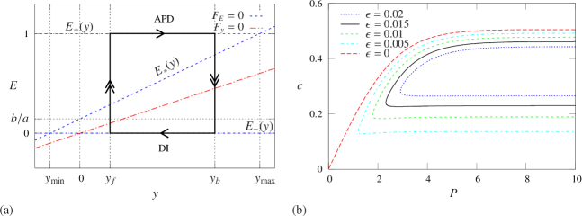
With this choice of the branches, assumptions A1 and A2 are satisfied for . However, assumption A3, specifically the condition , narrows this down to . The phase portrait and the N-shaped form of the reduced slow manifold of the Barkley model is illustrated in figure 1(a), with an example of a trajectory corresponding to a traveling wave train.
4.2 The fast subsystem
Substituting (27) into equations (25), (16) and (17) gives the front velocity
| (28) |
and the back velocity
| (29) |
As the front and the back have the same speed , we can obtain for a given by eliminating from system of equations (28) and (29) and resolving it with respect to , which gives
| (30) |
and provides a link for matching with the slow-time problem. The resulting interval of achievable speeds is .
4.3 The slow subsystem and matching
Evaluating expression (23) along the stable branches and of the reduced slow manifold given by (27), yields the temporal period of the wave
| (31) |
Combining expressions (28), (30) and (31), finally, yields the CV restitution curve in explicit form
| (32) |
which for gives the range . Figure 1(b) illustrates this result in comparison with curves obtained by numerical solution of the full boundary value problem (2) for equations (3) with right-hand sides given by (26) and periodic boundary conditions as described in section 2.
5 Asymptotic restitution curves in the FitzHugh-Nagumo model
5.1 The model
We will use the right-hand sides and of the FitzHugh-Nagumo equations in the following form,
| (33a) | |||
| (33b) | |||
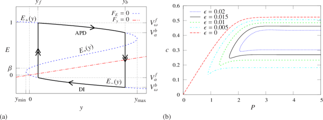
which is related to the original [23, 48] formulation by an affine transformation of the variables, involving the small parameter . Parameters and are assumed to obey , . The corresponding phase portrait is illustrated in figure 2(a), with a typical trajectory corresponding to a traveling wave train.
5.2 The fast subsystem
To use the general results on the front velocity (25), we need to know the branches of the reduced slow manifold and as functions of the slow variable . However, unlike the case of the Barkley model, here this would require using the formula for the roots of a generic cubic equation. This is rather inconvenient so we employ an alternative strategy. Given the value of the pre-front voltage at the lower branch of the reduced slow manifold, , we determine from equation (33a) the corresponding value of slow variable during the front . Further, to find the corresponding values of and the post-front voltage of the up-jump , we need to solve the cubic for which we already know one root, namely , so the cubic is divisible by . Hence the other two roots are solutions of the resulting quadratic equation, which leads to the required values
| (34a) | |||
| (34b) | |||
and therefore we get the expression for the front velocity
| (35) |
assuming , and a similar expression for the back velocity. Finally, from the condition we find the pre-back voltage as
| (36) |
which provides the link for matching with the slow-time system. The interval of bistability required by assumptions A1 and A2 in this case is , where with upper signs are for , lower signs are for , and . Assumption A3 narrows this to . Assumptions A4 and A5 for this interval are verified by direct elementary calculations, giving where .
5.3 The slow subsystem and matching
To use the coordinate to describe the motion along the reduced slow manifold, we rewrite (5) as
| (37) |
Therefore, we have the action potential duration as the time between and along the upper branch of the reduced slow manifold,
| (38) |
and the diastolic interval as the time between and along the lower branch of the reduced slow manifold,
| (39) |
and hence the period of the wave . Note that equations (38) and (39) have the same integrand, and only differ in the integration limits, which are related by relationship (34b), a similar expression relating and , and equation (36).
To summarize, equation (35) gives the wave velocity as the function of the pre-front voltage . Equation (36) gives the pre-back voltage as a function of the pre-front voltage . Equation (34b) and its analogue for the back give the post-front voltage and post-back voltage as functions of the pre-front voltage . Using those, finally, equations (38) and (39) give the wave period , as a function of the pre-front voltage . Hence, we have a parametric description of the conduction velocity restitution curve, in a parametric form with parameter the pre-front voltage . The parametric representation can be transformed into explicit representation by noting that expression (35) is equivalent to a quadratic equation with respect to the pre-front voltage and can be easily solved to give the desired explicit expression for as a function of ; the result, however, is rather lengthy and we omit it here.
Figure 2(b) presents a comparison between this explicit asymptotic dependence and the solution of the full periodic boundary-value problem at various values of .
6 Asymptotic restitution curves in the Caricature Noble model
The classical asymptotic theory of slow-fast systems described in the previous sections is not appropriate for the asymptotic reduction of cardiac equations which have a different nature, as pointed out in the Introduction. To develop a fully fledged alternative general theory is beyond the scope of this paper. Instead, in this section we study an archetypal “caricature” model of cardiac excitation previously proposed in [10]. One can think of this caricature model as a simple example of an ionic cardiac model in which a small parameter has been embedded so as to reveal explicitly the non-Tikhonov properties of the equations. The resulting fast and the slow problems have analytical solutions in closed form which makes the model convenient for investigation of well-posedness of the asymptotic reduction of the CV restitution problem in this particular case.
6.1 The model
We consider the following set of equations [10],
| (40a) | ||||
| (40b) | ||||
| (40c) | ||||
where
| (44) | |||
| (45) |
and where is the Heaviside unit step function.
The time in this model is measured in and the voltages , , , , , are measured in . Correspondingly, the units of , , are , and the units of , and are . As discussed above in section 2, the space scale is chosen to get the convenient value for the coefficient at the voltage diffusion term, so the dimensionality of in (40) is given by the “space unit” . The real physical lengths are given by where is the tissue voltage diffusion coefficient in the direction of wave propagation. The rest of the quantities in (40) are dimensionless.
This system is obtained from the authentic Noble model of Purkinje fibers [50] using a set of verifiable assumptions and well defined simplifications as detailed in [10]. The main features of equations (40) which make them an appropriate illustration are:
-
(a)
They reproduce exactly the asymptotic structure of the authentic Noble model [50], which is guaranteed by the embedding of the artificial small parameter . The authentic Noble model is the prototype of all contemporary voltage-gated cardiac models, and we believe that the asymptotic structure of (40) is rather generic in this class. Realistic voltage-gated cardiac models do not have explicit small parameters already present in them; or, rather, they have so many parameters that it is not a straightforward task which of them to use for asymptotics. Hence we employ a procedure of embedding artificial small parameters, as discussed e.g. in [10]. An example of the embedding procedure appears in section 7 below, where the Beeler-Reuter model [7] is discussed.
-
(b)
Equations (40) have the simplest possible functional form consistent with property (a). Most functions in the right-hand side are replaced by constants as justified in [10] which allows analytical solutions to be obtained in closed form. This in turn makes it possible to prove the well-posedness of the asymptotic boundary value problem to be formulated below.
For brevity, we shall call this model “Caricature Noble”.
6.2 The asymptotic reduction of the CV restitution boundary-value problem
Model (40) contains an explicit small parameter embedded in essentially the same way as it would be in a realistic model. In this section we demonstrate how this may be used for simplification of the Caricature Noble model or, indeed, of a more realistic ionic model.
A slow-time subsystem which describes the plateau and the recovery stages can be obtained immediately from equations (40), by taking the limit . At time scales much longer than , the second equation implies . Hence the first term of equation (40a) is proportional to which vanishes in the limit despite the large factor in front of it111 This is an attempt to summarize briefly the essence of the non-Tikhonov asymptotics of this and similar models. For a more detailed treatment, see our previous publications, e.g. [10]. . The diffusion term vanishes in the same limit and we are left with the slow-time system,
| (46a) | |||
| (46b) | |||
where is the traveling wave coordinate, which we use in this section instead of our standard choice of . A fast-time subsystem of equations (40) can be obtained by stretching time and space, , , taking the limit and neglecting the equation for which decouples from the rest. It is useful to distinguish explicitly the functions of the old from the functions of the new independent variables, say and . It is also useful to introduce at this stage the following non-dimensionalization (which, as noted above, is different from other sections and specific for this particular model)
| (47) |
In these variables, the travelling wave ansatz becomes . As a result of these transformations we obtain the following fast-time model of the wave front,
| (48a) | |||
| (48b) | |||
where . In a periodic wave train, a front propagates in the tail of the preceding wave, so slow pieces described by (46) and fast pieces described by (48) alternate, and there is one slow piece and one fast piece per period, as opposed to two fast pieces and two slow pieces in classical Barkley and FitzHugh-Nagumo models. The matching points for the van Dyke rule are: (a) the end of a slow piece corresponds to the beginning of the fast piece and (b) the end of the fast piece corresponds to the beginning of the next slow piece . This situation is summarized by the following set of boundary conditions
| (49a) | |||
together with
| (49b) | |||
where , , and are parameters to be found. Condition is a pinning condition as discussed above in (2), i.e. we choose . Condition follows from matching condition , by noting that in the slow time system is given by and . The asymmetry of the conditions imposed at can be understood by analysing the asymptotics of the linearized problem: the condition on the -derivative, , and the condition are satisfied automatically for open sets of solutions, whereas the the condition on the -derivative, , excludes solutions exponentially growing as and the condition excludes solutions exponentially growing as .
Equations (46) and (48) together with the boundary conditions (49) form a set of coupled boundary value problems representing an asymptotic description of CV restitution. The slow system is of order 2 while the fast system is of order 3 and there are 4 unknown constants namely , , and . Hence 9 conditions are needed to select a unique solution, while (49) provide only 8 conditions. Hence a one-parameter family of solutions may be found where the wave velocity is a function of the wave period, .
The asymptotic boundary-value problem (46),(48) and (49) of CV restitution is essentially simpler than the full one (2) for equations (40). Indeed, the small parameter has been eliminated and the resulting system is no longer stiff. Furthermore, the right-hand sides of equations are simpler and each stage of the action potential is modeled asymptotically by a system of lower dimension. However, to be useful the coupled asymptotic boundary value problem must satisfy two essential requirements: (a) the coupled problems must be well-posed (b) their asymptotic solution must provide a good approximation to the solution of the full non-asymptotic problem. It is not obvious that the asymptotic formulation of the CV restitution problem satisfies either of these requirements in the non-Tikhonov case under consideration. While a proof of properties (a) and (b) in the case of any arbitrary voltage-gated cardiac model is beyond the scope of this paper, in this section we prove the well-posedness of the archetypal Caricature Noble problem (46), (48) and (49). The convergence of the asymptotic and full solutions is demonstrated numerically.
6.3 The fast subsystem
6.3.1 Exact solution
To solve the fast-time equations (48) and (49a), we follow the ideas presented in [29, 56]. Since the right-hand-side of equation (48a) is a piece-wise function of voltage, we distinguish three intervals in terms of voltage separated by and 0, or alternatively in terms of the wave coordinate we use the intervals , and with internal boundaries and for which the equations and are satisfied, and impose natural continuity conditions at the internal boundaries. Exact analytical solution of the fast system can be obtained by first solving the -equation (48b) which is separable and independent of and then substituting its solution in the voltage equation (48a). In the first two intervals, and , equation (48a) is then readily solvable. The internal boundary point can be obtained by matching the solutions in these two intervals. To solve the voltage equation (48a) in the third interval we use the auxiliary change of variables,
| (50) |
and obtain a modified Bessel equation of order ,
| (51) |
the solutions of which are a linear superposition of the modified Bessel functions and of order [2]. The requirement of boundedness of the solution at infinity eliminates the term. The value of the post-front voltage is obtained as the limit of the expression for the voltage as and using formula [2, (9.6.7)]. In summary, the exact analytical solution of equations (48) is 222 At , , this solution coincides with that of Hinch [29] at .
| (52a) | |||
| (52b) | |||||
| (52c) |
where the internal boundary point is given by
| (53) |
and the post-front (peak) voltage is
| (54) |
where is the Gamma function [2]. The dispersion relation is then found from the continuity of the derivative of voltage at and takes the form
| (55) |
where the prime indicates a derivative with respect to the argument . At a given pre-front voltage , the wave velocity of the travelling impulses can be found as a solution of the dispersion relation (55) and we remind that for comparison with numerical results the wave velocity should be transformed back to the original variables, . Once again, note that the pre-front voltage cannot be found from conditions (49a) alone and so the entire front solution is a one-parameter function as expected.
The existence of solutions to the fast-time boundary value problem thus ultimately depends on the existence of solutions to the transcendental dispersion relation (55). Solutions are guaranteed by the following
Proposition 1
For every set of parameters such that and , there exists a unique value of the excitability parameter which solves (55).
Proof We will need an important property of modified Bessel functions: the ratio
is a strictly increasing function of its argument for any order . This follows directly from the estimate , [3, p. 243].
Moreover, it is easily established from the asymptotics of Bessel functions that and .
The right-hand side of (55) is a composite of the function
further depending on as a parameter, and the function
further depending on , and as parameters. In the assumptions made, is obviously strictly increasing as a function of , and maps . Using the recurrence relations [2, (9.6.26)], we can rewrite the definition of the function as
| (56) |
By and , we have that is strictly increasing (and therefore invertible) and maps . Overall, we conclude that the right-hand side of (55) is a strictly increasing function of defined for all and with the range of .
The left-hand side of (55) does not depend on the parameter and, since the pre-front voltage by assumption, it lies within which by is the range of the right hand side. Hence a solution always exists. Moreover, since by the right-hand side is strictly monotonic, the solution is unique.
Denoting by the inverse function to at the constant order , the existence of which has just been established in above, the solution of (55) can be written as
| (57) |
6.3.2 Bounds and asymptotics
We have demonstrated the existence of solutions to the fast subsystem (48) and (49a). We will now consider some estimates related to this solution which will lead to convenient explicit approximations of the propagation speed and the minimal excitability required for wave propagation. We treat as a parameter characterising the system (and omit dependence on it in the function notations), while and as variables characterising a particular front solution.
Lower bounds on the excitability
From and we know that , where the inequality becomes approximate equality for large . We shall denote this as . With account of (56), this implies that . A sharper upper bound, , is given in [3, (9)] and implies
| (58) |
Substituting this into (55), we get the more easily tractable approximation
| (59) |
Resolving this with respect to the excitability parameter , we get a lower bound for it in the form
| (60) |
The minimum of defined in (60) with respect to the wave speed at a constant pre-front voltage is achieved for
| (61) |
and is equal to
| (62) |
Hence, for any fixed value of the pre-front voltage and the excitability parameter , there exist two solutions for the wave speed , namely and .
Similarly, the minimum of with respect to the pre-front voltage for a fixed value of the wave speed is defined by
| (63) | |||
which is the negative root of the quadratic equation
| (64) |
and a corresponding value (the explicit equation for which is lengthy and of no further consequence so we omit it). Hence for any given wave speed , and excitability parameter , we have two solutions for the pre-front voltage , separated by the value .
Alternatively, equation (64) can be resolved with respect to to obtain
| (65) |
The absolute minimum of over is achieved when or, equivalently,
The left-hand side of this equation is a strictly decreasing function in , which is established e.g. by differentiation and using the estimate for (the calculations are tedious but elementary and we omit them). Besides, and , hence the above equation for the minimum always has a unique solution, , with corresponding and , all depending on as a parameter.
To summarize, we have established that the lower bound given by (60) has a unique absolute minimum in ), tends to infinity as and uniformly in and as and uniformly in . Hence by [43, Theorem 3.1], all level sets are diffeomorphic to each other, and thus are simple closed curves circumventing . Moreover, for any , there are two values of and , that are exactly two solutions of , such that for any , there exist exactly two solutions for the front velocity, and , where .
Estimates of the propagation velocity
Inequality (59) can also be explicitly resolved with respect to , giving double-sided inequality
| (66) |
where
| (67) |
| (68) |
and and are the principal and the alternate branch of the Lambert function [17], respectively.
The upper inequality in estimate (66) becomes an asymptotic equality for the faster velocity in the limit of rescaled coordinate which is achieved e.g. for large excitability and wave speed at fixed pre-front voltage . In this limit, the arguments of the Lambert functions are small, and since , , we have
| (69) |
which agrees with [29, (39)], as should be expected since in this limit the difference between our model and [29] is inessential.
Similarly, using a crude estimate for the alternate branch of Lambert function for , see [17], we find for the lower inequality in (66)
However, because the convergent series representation of the Lambert function is in terms of logarithms, it converges rather slowly, and thus the asymptotic above does not give a good approximation for the standard parameter values. A better, more accurate and simpler asymptotic can be obtained directly from (55) in the limit and using , , which can be easily obtained from [2, (9.6.7)]. This leads to
| (70) |
Note that since the estimate (70) is only asymptotic rather than uniform, it is not necessarily defined for all for which the solution exists. Indeed, since for all , we must require that in order that . This is only possible when , although according to (62), for , the minimal excitability .
6.3.3 On the properties of the exact solution
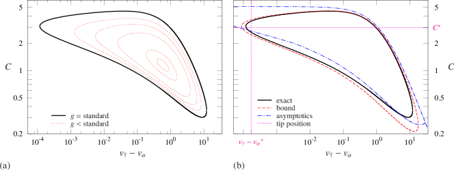
The above estimates of the propagation velocity are derived from the lower bound of the excitability . The exact dependence exhibits similar properties, as demonstrated numerically in in figure 3. We summarize these properties in the following
Conjecture 1
The function has an absolute minimum in , and for every the level set is a simple closed curve, crossing each line (or alternatively each line ) at most twice.
Supposing Conjecture 1 is true, the solutions of the dispersion relation form a simple closed curve, for every . Then there exist and with , such that for any equation (57) has two positive solutions for , which we may denote and , where . Since the level sets are simple closed curves the statement may be inverted so that has the role of the independent parameter: for every in some open interval there exist two distinct values of the pre-front voltage which satisfy equation (57). At the end points of the interval i.e. and equation (57) has single solutions for . The points and are extremum points of as a function of and the CV restitution curve has opposite slopes to the left and to the right of each of them.
The fast-time systems is linked, via the boundary conditions (49) and parameters and to the slow-time system the solution of which is discussed below.
6.4 The slow subsystem
The slow-time problem (46) and (49) can be solved exactly, too. Notice that it does not depend on the wave velocity and it is therefore similar to the slow problem considered in [10]. First, we solve equation (46b), which is separable and independent of . Its right-hand side is different in each of the two intervals due to the presence of a Heaviside function. The equation is constrained by the continuity condition at and periodic boundary conditions at and . The solution has the form
| (71) |
where the values of the constants and are different for the intervals () and () and are given in Table 1, and the overset index here above and below above designates the corresponding interval. This solution is then substituted in (46a) which becomes
| (72) |
where the constants , and also depend on the interval and are given in Table 1. The values in the table are obtained by a straightforward manipulation of the model definitions of and in (45) and the binomial theorem is used for the term . Within each of the intervals , and , equation (72) is a first order linear ODE with constant coefficients, and the solution of (46a) can be written in the explicit form,
| (73) |
where are integration constants. The exact solutions (71) and (73) contain seven parameters, namely , , , , , , , that need to be found from the boundary conditions and from the internal matching conditions,
| (74) | |||
The existence of solution to the slow-time boundary value problem ultimately depends on the existence of solutions of the transcendental equations (74). Based on the uniqueness and existence of solutions to an initial-value problem, it is obvious that the problem reduces to four essential unknowns, which we denote , , and .
Proposition 2
Suppose that the values of the parameters of the slow subsystem (46) and (49) obey the same qualitative relationships as the default values, i.e. , , and is continuous. Then for any and , the system of equations (71), (73), and (74) has a unique solution for and . For a fixed , this defines a function with domain and range , which is monotonically decreasing.
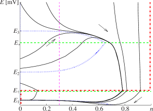
Proof is evident from the phase portrait shown in figure 4. Every trajectory starting above goes to the right and therefore eventually goes down below . Whilst below it goes to the left so as (this is also evident from the analytical solution). Therefore there exists a point such that . Moreover, such is unique, as the domain is absorbing and is monotonically increasing outside it and monotonically decreasing inside it. So we have the proposed mapping . The monotonicity of this mapping follows from the fact that the trajectories cannot intersect, so if , then the contour made by the straight line between points and and the segment of trajectory joining these two points, lies within the similar contour made by points and .
6.5 Matching and well-posedness
The CV restitution curve can be obtained by combining the results of the slow and the fast subsystems. According to Proposition 1 and Conjecture 1, for sufficiently large values of the excitability the fast subsystem defines the wave velocity as a function of prefront voltage, , for , which, via equation (54), defines the post-front voltage . On the other hand, according to Proposition 2, the wave period and the peak voltage are functions of and . Hence, the matching of the fast and slow solutions, for any given , can be obtained by solving the simultaneous system of equations for and , one resulting from the fast subsystem and one resulting from the slow subsystem, the latter depending on as a parameter. This subsequently provides where is given by the fast subsystem, and from the slow subsystem. Hence, we have ultimately the CV restitution curve in parametric form and we have proven that the asymptotic CV-restitution problem (46),(48) and (49) is indeed well-posed.
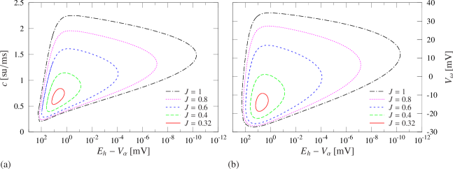
The equations of the aforementioned system for and are complicated and finding analytical solutions seems seems unfeasible. Some qualitative insight can be obtained from numerical analysis, which for the standard parameter values is illustrated in figure 5. The solutions correspond to the intersection of the closed fast-subsystem contour (dashed blue line) with a slow subsystem line (solid red lines). The family of slow-subsystem lines stretches continuously, but non-monotonically, from the vertical line at to the vertical line for . In accordance with Proposition 2, these lines are monotonically decreasing except for the above mentioned vertical lines for extreme values of . Almost all of these lines intersect the fast-subsystem contour, with the exception of the lines with very close to unity. The line , corresponds to the limit of the restitution curve, as that limit corresponds to a solitary wave propagating through the resting state, which is characterized by and . The other extremity corresponds to the line which is tangent to the slow-subsystem contour for a value of very close to but smaller than unity, and at a value of the pre-front voltage very close to but smaller than that of the parameter . As evident from the above analysis, e.g. see figure 3(a), we have as , which motivates consideration of asymptotics related to this limit. The details are presented in the next subsection.
Another qualitative feature evident from figure 5 is that the slow lines are nearly vertical for larger . This, and the non-monotonic behaviour of the horizontal () position of the slow-subsystem lines on around larger values of is a direct consequence of the non-monotonic behaviour of the trajectories which can be observed in figure 4: a typical “tail” of a trajectory starting at a large is a curve which starts at at , then decreases and then increases up until ; besides, all trajectories starting from larger join together very closely. As follows from the analysis in [10], this is due to an extra small parameter present in the slow subsystem, namely .
These observations motivate consideration of further asymptotics to the obtained solution, which lead to less accurate but more explicit results. We present them less formally than the main limit as they are of a secondary importance to our main results.
6.6 Further asymptotics
The fast branch of the restitution curve
For values of , the period is large compared to the parameter which plays the role of a time constant in the -gate equation (40c), and hence we can exploit the Tikhonov singular perturbation in terms of understood as a small parameter. This corresponds to the secondary asymptotic embedding considered in [10]. In this limit, the trajectories differ only in the initial post-overshot stage, after which they move along the reduced superslow manifold with the exception of the repolarization stage when . It is important to note that except during the the initial transient, the trajectories are nearly the same, up to a correction which is exponentially small in as evident from figure 4. We consider two parts of a typical trajectory, one for when increases, and the other for when it decreases. Due to the above mentioned convergence of trajectories, the value is practically independent on up to exponentially small corrections. A typical value of can be found e.g. in the following way: first, consider solution (73) for and and solve the matching condition for , next determine from the initial condition , then solve for , and finally with the knowledge of and , the value of can be obtained from (71) as . This however leads to a transcendental equation. Numerical value for the standard parameter values is .
Using (71), the duration of the second half of the trajectory, between , , and , , , is given by
| (75) |
The evolution of during the second half of a typical slow trajectory, is described by the relevant form of equation (46a)
wherefrom
| (76) |
Combining (75), (76) and (69), we get an explicit dependence of in elementary functions.
The slow branch of the restitution curve
The slow branch is considered in a similar way. The difference is in the initial transient where a typical trajectory approaches the reduced superslow manifold from lower values of rather than from the higher as it was for the faster branch, and also in the dependence. Hence the dependence of is obtained by combining (75), (76) and (70).
The turning point of the restitution curve
The turning point is the point where the fast branch meets the slow branch. It is characterized by extreme proximity of to and to 1. The front parameters can be estimated via the limit , of (61) and (62), which gives the highest pre-front voltage as
| (77) |
and the corresponding slowest stable front velocity as
| (78) |
Given and , equation (54) then gives the value of the post-front voltage,
| (79) | |||
| (80) |
The duration of the slow trajectory corresponding to these and will be an estimate of the shortest wave period possible in this model, . A simple approximation of it can be obtained from the consideration that in the limit , we have throughout, hence the slow-subsystem equation for is simplified by replacing so the link between and dynamics is only via the values of and . The period is almost the same as the taken by the voltage to decrease from to , since the interval needed to decrease from to is small compared to that. In this case, the interval can be estimated from solutions (73) for . Hence, we have
| (81) |
Equations (77)–(81), together with the scaling relationships (47) define the turning point of the restitution curve. For the standard parameter values, this gives
| (82) |
6.7 Comparison of the asymptotics with the exact solution
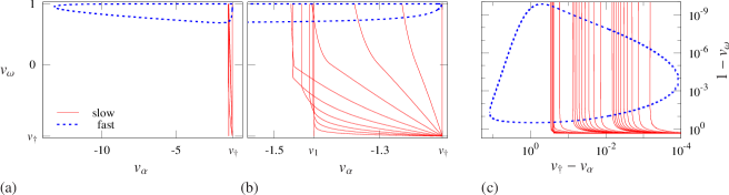
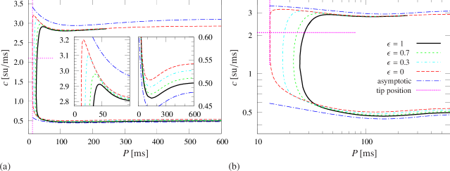
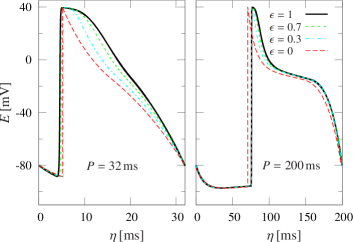
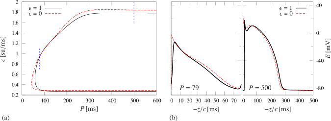
With the aim to assess the proximity of the analytical solutions obtained in the main asymptotic limit and the full numerical solutions of the CV restitution boundary value problem, we present in figure 6 sets of CV restitution curves of the Caricature Noble model, and we show in figure 7 the action potential profiles for two selected base cycle lengths . We also demonstrate in figure 6 the asymptotic estimates of the upper and lower branches and of the tip position of the curve found with the help of the secondary embedding . The asymptotic CV restitution curve was obtained by solving numerically problem (46), (48) and (49) which defines and . The full CV restitution curve was obtained by solving the full boundary-value problem (2) formulated for equations (40). Figure 6(a) presents the curves in Cartesian coordinates and figure 6(b) in semi-logarithmic coordinates to reveal in more details the behaviour at small values of the wave period . We can see that as is decreased the solution of the full problem converges to the solution of the asymptotically reduced problem at , and that the full model curve for at standard parameter values is close to the asymptotic limit everywhere except at the smallest values of the period .
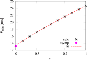
This indicates that at small , the parameter is not a “good small parameter”. Note that in our asymptotic analysis, we have calculated the period as the length of the slow subsystem solution, and we have neglected the contribution of the fast subsystem, i.e. the duration of the front, which is small of the order . However, at the smallest values of , the the front length is comparable to duration of the solution of the slow subsystem. This can be seen already in figure 6 and figure 7, and is further confirmed by the analysis of the dependence of the minimal wave period on shown in figure 8. We see that to second order, the basic cycle length can be approximated by , where is the cycle length given by the asymptotic theory presented above, and may be interpreted as the front duration in the fast subsystem. Note that , hence neglecting for smaller produces relatively large error. That this is not the whole story, however, as not only the horizontal position of the point changes with , but also its vertical position , so a proper next-order asymptotic should take into account of the influence of the slow subsystem on the front velocity as well.
7 Asymptotic restitution curves in the Beeler-Reuter model
In this section we apply the methodology presented above to the Beeler-Reuter ventricular model [7]. This model is an example of a realistic voltage-gated model which represents an intermediate step between relatively simple early models and complicated contemporary models. It has played an important role for understanding of cardiac excitability with a large volume of literature devoted to it, and it is still the model of choice in many situations, e.g. [21, 28, 14] are some recent examples. In the following, we find the CV restitution curve of the Beeler-Reuter model using both the asymptotic formulation and the full formulation of the periodic boundary value problem as described above and demonstrate an excellent quantitative agreement.
7.1 The model and the asymptotic embedding
The initial step of our approach requires an appropriate asymptotic embedding of the original Beeler-Reuter model [7]. The embedding is constructed following the procedures presented in detail in our earlier works [12, 56, 10] and here we shall summarize briefly the relevant arguments. We would like to remark that an analogous embedding procedure applies to the Caricature Noble model of section 6 where appeared seemingly without much justification.
We rewrite the Beeler-Reuter model in the one-parameter form,
| (83a) | |||
| (83b) | |||
| (83c) | |||
| (83d) | |||
where only the equations affected by the artificial small parameter are shown. As in the previous model, the voltage is measured in , time in , the gating variables , , , are non-dimensional, and the space coordinate is measured in .
The functions and are time-scaling functions and quasi-stationary values of the gating variables, respectively. Functions and are “embedded”, i.e. they are -dependent versions of and such that and on one hand and and on the other hand, with and so that and . The last two parameters are analogous to and of the Caricature Noble model. The rest of the model (83) is the same as defined in [7], namely is the sum of all slow currents, is the vector of all slow variables in addition to gate which is also slow, and stands for the functions governing the dynamics of the gating variables . The rationale for this parameterisation is the following.
-
1.
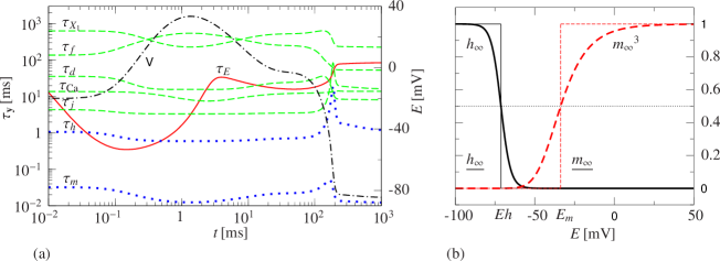
The dynamic variable is a ‘superfast’ variable and has been adiabatically eliminated by replacing it with its quasi-stationary value . The variables and are ‘fast variables’, i.e. they change significantly during the upstroke of a typical AP potential, unlike all other variables which change only slightly during that period. The relative speed of the dynamic variables is estimated by comparing the magnitude of their corresponding ‘time-scaling functions’ as illustrated in figure 9(a). For a system of differential equations , the time scale functions are defined as , and coincide with the functions already present in (83).
-
2.
The dynamic variable is fast due only to one of the terms in the right-hand side, the large sodium current , whereas other currents are not that large and so do not have the large coefficient in front of them.
-
3.
The fast sodium current is large only during the upstroke of the AP, and not that large otherwise. This is due to the fact that either gate or gate or both are almost closed outside the upstroke since their quasistationary values and are small there as seen in figure 9(b). Thus in the limit , functions and have to be considered zero in certain overlapping intervals and , and , hence the representations and .
A more detailed discussion of the parameterisation given by (83), as well as the justification of our method of parametric embedding, i.e. a seemingly “arbitrary” introduction of an artificial small parameter , can be found in [10].
7.2 The asymptotic reduction
We are now ready to formulate the asymptotic CV restitution problem as a set of coupled boundary value problems similar to those described in section 6.2. Being interested in propagation with constant velocity and fixed shape, we introduce the travelling wave coordinates for the slow subsystem and for the fast subsystem. As before, we distinguish the functions of the fast time by name and set and .
The slow-time subsystem is obtained in the limit of the original slow independent variable ,
| (84a) | |||
| (84b) | |||
| (84c) | |||
| (84d) | |||
The fast-time subsystem is obtained in the limit of the fast independent variable ,
| (85a) | |||
| (85b) | |||
| (85c) | |||
The boundary conditions of the fast subsystem include the pinning condition eliminating the translational invariance along the axis. This problem depends on four parameters, namely the pre-front voltage , the post-front voltage , the fixed value of the gate inherited from the slow system and the wave speed which are determined by matching with the slow subsystem, given by the conditions,
| (86) |
7.3 The fast subsystem
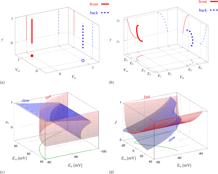
The fast subsystem (85) describes the wave front of an action potential as it propagates by diffusion. This problem has, on one hand, differential equations of cumulative order three and four parameters, and on the other hand, five constraints, thus the solution will typically depend on two “leading” parameters chosen arbitrarily, and the other parameters will be functions of these two. The structure of the equations (85) is very similar to the fast subsystem of the Caricature Noble model (48) and (49a). In fact, if was a piecewise constant function with a step at , then the Beeler-Reuter fast subsystem would be equivalent to the Caricature Noble fast subsystem up to parameter values and identification of in the former with in the latter. Hence we may expect that the set of solutions here has a structure similar to that of the Caricature Noble model. In particular, we expect that and can be determined as univalued functions of and . Further, we expect that for a fixed , we have the set of solutions in the such that there exists such that if then there exists an interval such that for any within this interval, there are two solutions for the front velocity , and correspondingly two values of the postfront voltage . This is confirmed by numerical analysis of this problem, see figure 10.
7.4 The slow subsystem
As in the Caricature Noble model, the slow subsystem in the leading order does not depend on diffusion, and therefore coincides, up to the scaling of the independent variable, with the slow subsystem of the single-cell model. The slow subsystem depends on four parameters, namely the pre-front voltage , the post-front voltage , the initial value of the -gate and the wave period , and has differential equations of cumulative order of . On the other hand it has constraints, hence, similarly to the fast system, it has typically a two-parametric family of solutions. From the viewpoint of matching with the fast-time problem and in analogy with the Caricature Noble case, one possible convenient choice of leading parameters is and from which , as well as can be found. However, unlike the Caricature Noble case, it is now more difficult to establish rigorous conditions for existence of solutions. This, however, can be easily done numerically.
7.5 Matching and comparison with the exact solution
The three constraints (86) offset the four free parameters of the slow and fast subsystems so that the resulting set of solutions is typically one-parametric, i.e. it is curve in the parameter space. The projection of this curve on the is the CV restitution curve. Given appropriate analytical approximation of the relevant dependencies, which could be obtained for instance by asymptotic means or by fitting, solving the resulting finite (transcendental) system will produce analytical approximation for the restitution curve. Doing so for Beeler-Reuter model is however beyond the scope of this paper and we restrict to demonstrate the validity of our asymptotic approach for this model by solving the asymptotic matching problem numerically.
In solving the problem (84), (85) and (86) numerically, the following features need to be taken into account
-
(a)
The fast-time problem is posed on an infinite interval.
-
(b)
At the same time the slow-time system is posed on a finite interval.
-
(c)
The length of that finite interval is the wave length of the periodic travelling wave, i.e. it is an unknown variable.
-
(d)
The fast-time system has piece-wise right-hand sides.
-
(e)
The pinning condition needs to be imposed in the fast subsystem. Since the fast system is piece-wise, it is convenient to impose it at a boundary between pieces.
-
(f)
The slow variable appears as a parameter in the fast-time system.
These features can be addressed by a number of well-known techniques and we refer the interested reader to [5] for a general discussion and to [56] for a numerical implementation of a similar problem. In short, the issue of the boundary conditions at infinity can be resolved by considering a finite interval with boundary conditions obtained as a solution of the problem linearised about the asymptotic equilibria. This finite interval is then dissected into three subintervals to take care of the piece-wise definition of the equations. The three subinterlals together with the interval on which the slow-time system is posed are then mapped to the interval by introducing appropriate scaling factors. The pinning condition can be easily incorporated at one of the internal matching points. Finally, in this representation equations (85)–(86) can be solved by any standard boundary value problem solver such as Maple’s dsolve [63], NAG’s d02raf [47] and others.
The resulting asymptotic CV restitution curve is shown in figure 11 by a dashed thin red line. The bold solid black line in the figure corresponds to the CV restitution curve found from the full non-asymptotic boundary value problem (2) written for the full Beeler-Reuter model (83) at . The two curves demonstrate a good quantitative agreement.
We would like to emphasize here that, while it was still possible to solve the full problem numerically in this case, and the asymptotic problem was solved numerically too, solution of the full problem was a substantially more difficult task than the computation of the asymptotic CV restitution curve. The problem is certainly well-posed but it is very stiff and it required a prolonged experimentation with a variety of software tools and parameter continuation techniques. It is also worth recalling that the Beeler-Reuter model is not as complicated as contemporary models are, which leads us to expect that the non-asymptotic problem for such models is even more difficult to solve.
8 Discussion
Summary
We have demonstrated that singular perturbation theory based on the largeness of the maximal value of the sodium current compared to other currents and quality of the ionic gates (smallness of and in certain voltage ranges), is capable of reproducing essential spatiotemporal phenomena, using conduction velocity restitution curve as the simplest nontrivial example involving both the fast scale and slow scale. We have explicitly compared the mathematical technique involved here, with similar problems in the classical FitzHugh-Nagumo (FHN) like models of excitable media. Apart from the different number of equations and the more complicated right-hand sides, we have identified in the cardiac models qualitatively new features of topological nature.
Classical simplified excitable models vs ionic cardiac models
Figure 12 illustrates the fundamental difference between FHN-like and cardiac models as far as the problem of and selection is concerned. In FHN-like systems (panels (a) and (b)), if the values of the slow variables are given, then and are uniquely defined, up to the choice between front (jump up) and back (jump down). So, for one slow variable as in the examples considered in section 3, there are one-dimensional manifolds representing all possible fronts and backs. In contrast in cardiac equations (panels (c) and (d), we have two-dimensional manifolds in place of one-dimensional manifolds. This is related to the fact that in the parametric embedding we use, the transmembrane voltage, like a double-faced Janus, is both a “slow” and a “fast” variable. In its slow capacity, it contributes to the pre-front conditions, among other slow variables. In its fast capacity, it participates in the excitation front. So given one “truly slow” variable ( in panel (c) and in panel (d)), we have not a one-dimensional, but a two-dimensional manifold representing possible fronts, as even when the value of that slow variable is fixed, the prefront voltage and, consequently, post-front voltage are still undefined. Hence to obtain the restitution curve, which is a 1-dimensional manifold, we have to find an intersection of the manifold representing possible fast fronts with the manifold representing possible slow solutions, which is something that we don’t do for the FHN-like systems.
Another qualitative difference is, of course, the number of fast solutions per one excitation pulse. In FHN-type systems, it is essential that there is a back corresponding to every front, as the systolic and diastolic pieces of the reduced slow manifold are separated from each other. In our asymptotic embedding of cardiac models, the systolic and diastolic pieces of the slow set (which is now not a manifold) are connected via a piece where both and gates are firmly closed and is in its slow-variable capacity. Here it should be noted that existence of a back is not a necessary feature of a FHN-type system, as in presence of two or more slow variables it is possible to have a slow manifold with a cusp singularity so that its systolic and diastolic pieces of the are connected via a monostable pieces, as in the example suggested by Zeeman [65]. However, although the structure of ionic models admits, in principle, such manifolds [57], it has not been identified in any cardiac models so far.
The numerical method for dynamic CV restitution curves
In this work, we have proposed a computationally efficient method of calculating an ideal case of the so called “dynamic” or “steady-state” restitution protocol, with exactly periodic propagating pulses. The method exploits asymptotic splitting the problem into two parts, the slow and the fast subsystems. The advantage of such a split is that each of the subsystems no longer depends on the small parameter due to the largeness of and quality of its ionic gates, so they are significantly less stiff than the original full problem, hence the computational efficiency. The well-posedness of the problems arising from the asymptotic splitting is not obvious a priori, since the asymptotic embedding we use is non-Tikhonov, and the general results from singular perturbation theory are not applicable to our case. We have thus taken care to prove the well-posedness, at least for the case considered.
Perspectives: more complicated spatiotemporal regimes
There are several other protocols used in defining restitution curves, see e.g. [54] and references therein. They do not correspond to periodic steadily propagating wave solutions. Nevertheless, we expect that the proposed asymptotic splitting should still work there, under some natural assumptions.
So, if propagation of waves is not too complicated, then evolution of the system away from the fronts can be expected to be well approximated by the corresponding slow subsystem, which is a non-stiff ordinary differential equation for every point of the medium. After application of the propagating wave ansatz, the slow subsystems of the Caricature Noble and Beeler-Reuter become systems (46) and (84) respectively. Here we note, that without such ansatz, the slow subsystems would be differential equations with time as the independent variable, with exactly the same structure as (46) and (84) only with a different scaling, so all the above analysis applies. Fronts themselves for most part of their evolution can be considered locally as steadily propagating nearly plane waves, well described by systems like (48) and (85).
Under these assumptions, according to the analysis of the fast subsystem, the conduction velocity and post-front voltage can be found as functions of the pre-front voltage and, if relevant, pre-front value of gate , and the dynamics of the front is governed by an ordinary (in the case of one spatial dimension) differential equation for the position of the front as a function of time. This gives an unusually coupled system of ordinary differential equations: the local dynamics provide right-hand sides for the equation of motion of the next front, and trajectory of the front provides initial condition for the subsequent piece of slow dynamics. This unusual ODE system can predict non-stationary evolution of the excitation patterns, including restitution protocols. In different settings, this approach has been used e.g. in [11] and [22]. As demonstrated in [22], such unusually coupled ODE system can form a basis for investigation of such complicated spatiotemporal phenomenon as the spatiotemporal dynamics of cardiac alternans. 333 Echebarria and Karma [22] considered a simplified model with some features of the ionic models and similar to the Caricature Noble model considered there, but only two variables, without any slow gates. So extension of the present results to other, more complicated and important spatiotemporal regimes, seems to be a natural and imminent next step.
Perspective: the problem of restitution memory
The above considerations lead us to the problem of rate-dependence of restitution curves, or the so called “memory” effects, see e.g. [54] and references therein. A typical approach to studying memory effects is purely phenomenological: memory variables in the restitution relationships are usually postulated and their properties are obtained inductively from measurements of the differences between results from various restitution protocols. Asymptotic analysis such as the one used in the present work offers a deductive ab initio way of treatment of the memory variables. In such setting, the number of memory variables equals dimensionality of the phase space of the slow subsystem minus one, and the memory variables themselves may be identified with values of the slow variables apart from , measured during an excitation front. For example, in the Caricature Noble model here there would be one memory variable, say taken to be , and in the Beeler-Reuter model, there would be of them, and they may be identified with the values of the slow variables , , and as measured at the front, thus making the restitution much more difficult to predict. However, empirical evidence from simulations of modern detailed ionic models suggests that variety of slow trajectories may be much narrower, i.e. they may de facto be restricted to a manifold of a smaller dimensionality [56]. A possible theoretical explanation for such dimensionality reduction is the presence of further small parameters within the slow subsystem; this mechanism was considered in detail in [10]. So detailed studies of finer asymptotic structure of slow subsystems of practically interesting ionic models are a promising direction for further studies, which may help in understanding the memory effects in restitution. It is well known that memory effects can play considerable part in development of alternans and therefore in development of cardiac arrhythmias (see e.g. [44] for a recent study) and are for this reason of considerable interest.
Perspective: a novel numerical method for excitation propagation
The above considerations outline possible qualitative applications of the present study. A possible quantitative application is an advanced method for calculation of activation sequences, which can be achieved by the aforementioned coupling of differential equations for the local slow dynamics and for the front motion. For these applications, two or three spatial dimensions rather than one are interesting, hence the equation of motion for the front is a partial differential equation of motion of a line (in 2D) or surface (in 3D). One immediate difference is that propagation of the front shall no longer depend only on the prefront voltage and -gate, but also on the spatial configuration of the front. It is well known that unless the shape of the front deviates very strongly from plain, the effect of its shape is mostly accounted for through its mean curvature, and we have demonstrated that the effect of curvature can be easily incorporated into the asymptotic description of the front dynamics [56]. This approach can be used to describe normal activation sequences in the heart, when the graph of the front solution in the space-time is a manifold without internal boundaries. More serious problems occur if there are propagation blocks and/or wave breaks, which introduce boundaries of the front manifold in space-time. In such cases, a separate asymptotic description for the codimension-two areas, the wave break trajectories and the propagation block loci, are needed; obtaining such asymptotic description is another important direction for further research.
An obvious caveat here is, as with any asymptotic approach, that the asymptotics are valid in the limit of whereas we apply it for a finite value of that small parameter. Hence applicability of this approach on the quantitative level will depend on whether the error generated by such approximation is tolerable for the particular application; however, it should be remembered that higher-order terms if necessary can improve the accuracy, see an example in [10].
References
- [1]
- Abramowitz and Stegun [1965] Abramowitz, M. and Stegun, I. A., eds [1965], Handbook of mathematical functions: with formulas, graphs, and mathematical tables, Dover, New York.
- Amos [1974] Amos, D. E. [1974], ‘Computation of modified bessel functions and their ratios’, Mathematics of Computation 28(125), 239–251.
- Aronson and Weinberger [1978] Aronson, D. G. and Weinberger, H. F. [1978], ‘Multidimensional non-linear diffusion arising in population genetics’, Advances in Mathematics 30(1), 33–76.
- Ascher and Russell [1981] Ascher, U. and Russell, R. D. [1981], ‘Reformulation of boundary value problems into “standard” form’, SIAM Review 23, 238–254.
- Barkley [1991] Barkley, D. [1991], ‘A model for fast computer simulation of waves in excitable media’, Physica D 49, 61–70.
- Beeler and Reuter [1977] Beeler, G. W. and Reuter, H. [1977], ‘Reconstruction of the action potential of ventricular myocardial fibres’, J. Physiol. Lond. 268, 177–210.
- Biktashev [2002] Biktashev, V. N. [2002], ‘Dissipation of the excitation wavefronts’, Phys. Rev. Lett. 89(16), 168102.
- Biktashev and Suckley [2004] Biktashev, V. N. and Suckley, R. [2004], ‘Non-Tikhonov asymptotic properties of cardiac excitability’, Phys. Rev. Lett. 93(16), 168103.
- Biktashev et al. [2008] Biktashev, V. N., Suckley, R. S., Elkin, Y. E. and Simitev, R. D. [2008], ‘Asymptotic analysis and analytical solutions of a model of cardiac excitation’, Bull. Math. Biol. 70(2), 517–554.
- Biktashev and Tsyganov [2005] Biktashev, V. N. and Tsyganov, M. A. [2005], ‘Solitary waves in excitable systems with cross-diffusion’, Proc. Roy. Soc. Lond. ser. A 461(2064), 3711–3730.
- Biktasheva et al. [2006] Biktasheva, I. V., Simitev, R. D., Suckley, R. S. and Biktashev, V. N. [2006], ‘Asymptotic properties of mathematical models of excitability’, Phil. Trans. Roy. Soc. Lond. ser. A 364(1842), 1283–1298.
- Boyett and Jewell [1978] Boyett, R. and Jewell, B. R. [1978], ‘A study of the factors responsible for rate-dependent shortening of the action potential in mammalian ventricular muscle’, J. Physiol. Lond. 285, 359–380.
- Chen et al. [2007] Chen, W., Potse, M. and Vinet, A. [2007], ‘Dynamics of sustained reentry in a loop model with discrete gap junction resistances’, Phys. Rev. E 76, 021928.
- Chialvo et al. [1990] Chialvo, D. R., Michaels, D. C. and Jalife, J. [1990], ‘Supernormal excitability as a mechanism of chaotic dynamics of activation in cardiac Purkinje fibers’, Circ. Res. 66, 525–545.
- Clayton [2001] Clayton, R. H. [2001], ‘Computational models of normal and abnormal action potential propagation in cardiac tissue: linking experimental and clinical cardiology’, Physiol. Meas. 22, R15–R34.
- Corless et al. [1996] Corless, R. M., Gonnet, G. H., Hare, D. E. G., Jeffrey, D. J. and Knuth, D. E. [1996], ‘On the Lambert W function’, Adv. Comp. Math. 5, 329–359.
- Courtemanche [1996] Courtemanche, M. [1996], ‘Complex spiral wave dynamics in a spatially distributed ionic model of cardiac electrical activity’, Chaos 6, 579–600.
- Courtemanche et al. [1993] Courtemanche, M., Glass, L. and Keener, J. P. [1993], ‘Instabilities of a propagating pulse in a ring of excitable media’, Phys. Rev. Lett. 70, 2182–2185.
- Dockery and Keener [1989] Dockery, J. D. and Keener, J. P. [1989], ‘Diffusive effects on dispersion in excitable media’, SIAM J. Appl. Math. 49(2), 539–566.
- Dokos and Lovell [2004] Dokos, S. and Lovell, N. H. [2004], ‘Parameter estimation in cardiac ionic models.’, Prog. Biophys. Mol. Biol. 85, 407–431.
- Echebarria and Karma [2007] Echebarria, B. and Karma, A. [2007], ‘Amplitude equation approach to spatiotemporal dynamics of cardiac alternans’, Phys. Rev. E 76, 051911.
- FitzHugh [1961] FitzHugh, R. [1961], ‘Impulses and physiological states in theoretical models of nerve membrane’, Biophysical Journal 1, 445–456.
- Garfinkel et al. [2000] Garfinkel, A., Kim, Y. H., Voroshilovsky, O., Qu, Z., Kil, J. R., Lee, M. H., Karagueuzian, H. S., Weiss, J. N. and Chen, P. S. [2000], ‘Preventing ventricular fibrillation by flattening cardiac restitution’, Proc. Natl. Acad. Sci. USA 97, 6061–6066.
- Gorban and Karlin [2005] Gorban, A. N. and Karlin, I. V. [2005], ‘Invariant Manifolds for Physical and Chemical Kinetics’, Springer Lect. Notes Phys. 660.
- Hakim and Karma [1999] Hakim, V. and Karma, A. [1999], ‘Theory of spiral wave dynamics in weakly excitable media: Asymptotic reduction to a kinematic model and applications’, Phys. Rev. E 60(5), 5073–5105.
- Heineken et al. [1967] Heineken, F. G., Tsuchiya, H. M. and Aris, R. [1967], ‘On the Mathematical Status of the Pseudo-steady State Hypothesis of Biochemical Kinetics’, Mathematical Biosciences 1, 95–113.
- Herman et al. [2007] Herman, D., Prevorovska, S. and Marsik, F. [2007], ‘Determination of myocardial energetic output for cardiac rhythm pacing’, Cardiovasc. Eng. 7, 156–161.
- Hinch [2002] Hinch, R. [2002], ‘An analytical study of the physiology and pathology of the propagation of cardiac action potentials’, Prog. Biophys. Mol. Biol. 78, 45–81.
- Hodgkin and Huxley [1952] Hodgkin, A. L. and Huxley, A. F. [1952], ‘A quantitative description of membrane current and its application to conduction and excitation in nerve’, J. Physiol. Lond. 117, 500–544.
- http://www.physiome.org [n.d.] http://www.physiome.org [n.d.].
- Ito and Glass [1992] Ito, H. and Glass, L. [1992], ‘Theory of reentrant excitation in a ring of cardiac tissue’, Physica D 56, 84–106.
- Jones [1995] Jones, C. K. R. T. [1995], ‘Geometric Singular Perturbation Theory’, Springer Lect. Notes in Math. 1609, 44–118.
- Kaper and Kaper [2002] Kaper, H. G. and Kaper, T. J. [2002], ‘Asymptotic analysis of two reduction methods for systems of chemical reactions’, Physica D 165, 66–93.
- Kaper [1999] Kaper, T. J. [1999], ‘An introduction to geometric methods and dynamical systems theory for singular perturbation problems’, AMS Proceedings of Symposia in Applied Mathematics 56, 85–132.
- Karma [1994] Karma, A. [1994], ‘Electrical alternans and spiral wave breakup in cardiac tissue’, Chaos 4, 461–472.
- Karma et al. [1994] Karma, A., Levine, H. and Zou, X. [1994], ‘Theory of pulse instabilities in electrophysiological models of excitable tissues’, Physica D 73,, 113–127.
- Keener [1980] Keener, J. P. [1980], ‘Waves in excitable media’, SIAM J. Appl. Math. 39(3), 528–548.
- Keener [1991] Keener, J. P. [1991], ‘The effects of discrete gap junction coupling on propagation in myocardium’, J. theor. Biol 148, 49–82.
- Keener and Sneyd [1991] Keener, J. P. and Sneyd, J. [1991], Mathematical Physiology, Springer, Berlin.
- McKean [1970] McKean, H. P. [1970], ‘Nagumo’s equation’, Advances in Mathematics 4, 209–223.
- Meron [1992] Meron, E. [1992], ‘Pattern formation in excitable media’, Phys. Rep. 218(1), 1–66.
- Milnor et al. [1963] Milnor, J. W., Spivak, M. and Wells, R. O. [1963], Morse theory, Princeton University Press.
- Mironov et al. [2008] Mironov, S., Jalife, J. and Tolkacheva, E. G. [2008], ‘Role of conduction velocity restitution and short-term memory in the development of action potential duration alternans in isolated rabbit hearts’, Circulation 118(1), 17–25.
- Mishchenko and Rozov [1980] Mishchenko, E. F. and Rozov, N. K. [1980], Differential Equations with Small Parameters and Relaxation Oscillations, Plenum Press, New York.
- Murray [1991] Murray, J. D. [1991], Mathematical Biology, Springer, Berlin.
- NAG [Mark 20] NAG [Mark 20], ‘The Numerical Algorithms Group, Ltd. Fortran Library Manual’.
- Nagumo et al. [1962] Nagumo, J., Arimoto, S. and Yoshizawa, S. [1962], ‘An active pulse transmission line simulating nerve axon’, Proc. IRE 50, 2061–2070.
- Noble [1960] Noble, D. [1960], ‘Cardiac action and pacemaker potentials based on the Hodgkin-Huxley equations’, Nature 188, 495–497.
- Noble [1962] Noble, D. [1962], ‘A modification of the Hodgkin-Huxley equations applicable to Purkinje fibre action and pace-maker potentials’, J. Physiol. Lond. 160, 317–352.
- Nolasco and Dahlen [1968] Nolasco, J. B. and Dahlen, R. W. [1968], ‘A graphic method for the study of alternation in cardiac action potentials’, J. Appl. Physiol. 25, 191–196.
- Plank et al. [2006] Plank, G., Clayton, R., Boyd, D. and Vigmond, E. [2006], ‘Integrative biology: modelling heart attacks with supercomputers’, Capability Computing. The newsletter of the HPCx community 7, 4–9.
- Pontryagin [1957] Pontryagin, L. S. [1957], ‘The asymptotic behaviour of systems of differential equations with a small parameter multiplying the highest derivatives’, Izv. Akad. Nauk SSSR, Ser. Mat. 21(5), 107–155.
- Schaeffer et al. [2007] Schaeffer, D., Cain, J., Gauthier, D., Kalb, S., Oliver, R., Tolkacheva, E., Ying, W. and Krassowska, W. [2007], ‘An ionically based mapping model with memory for cardiac restitution’, Bull. Math. Biol. 69, 459–482.
- Segel and Slemrod [1989] Segel, L. A. and Slemrod, M. [1989], ‘The Quasi-Steady-State Assumption: A Case Study in Perturbation’, SIAM Review 31, 446–477.
- Simitev and Biktashev [2006] Simitev, R. D. and Biktashev, V. N. [2006], ‘Conditions for propagation and block of excitation in an asympthotic model of atrial tissue’, Biophysical Journal 90, 2258–2269.
- Suckley and Biktashev [2003] Suckley, R. and Biktashev, V. N. [2003], ‘The asymptotic structure of the Hodgkin-Huxley equations’, Int. J. of Bifurcation and Chaos 13(12), 3805–3826.
- Tikhonov [1952] Tikhonov, A. N. [1952], ‘Systems of differential equations, containing small parameters at the derivatives’, Mat. Sbornik 31(3), 575–586.
- Tyson and Keener [1988] Tyson, J. J. and Keener, J. P. [1988], ‘Singular perturbation theory of traveling waves in excitable media’, Physica D 32, 327–361.
- van der Pol [1920] van der Pol, B. [1920], ‘A theory of the amplitude of free and forced triode vibrations’, Radio Review 1, 701–710.
- Watanabe et al. [2001] Watanabe, T., Fenton, F., Evans, S., Hastings, H. and Karma, A. [2001], ‘Mechanisms for discordant alternans’, J. Cardiovasc. Electrophysiol. 12, 196–206.
- Watanabe et al. [1995] Watanabe, T., Rautaharju, P. M. and McDonald, T. F. [1995], ‘Ventricular action potentials, ventricular extracellular potential, and the ECG of guinea pig’, Circ. Res. 57, 362–373.
- Waterloo Maple Inc. [Version 11] Waterloo Maple Inc. [Version 11], ‘Maple’.
- Zagaris et al. [2004] Zagaris, A., Kaper, H. G. and Kaper, T. J. [2004], ‘Analysis of the Computational Singular Perturbation Reduction Method for Chemical Kinetics’, J. Nonlin. Sci. 14, 59–91.
- Zeeman [1972] Zeeman, E. C. [1972], Differential Equations for the Heartbeat and Nerve Impulse, Mathematics Institute, University Of Warwick, Coventry.
- Zel’dovich and Frank-Kamenetsky [1938] Zel’dovich, Y. B. and Frank-Kamenetsky, D. A. [1938], ‘Towards the theory of uniformly propagating flames’, Doklady AN SSSR 19, 693–697.