Particle-Hole Asymmetry and Brightening of Solitons in a Strongly Repulsive BEC

Abstract

We study solitary wave propagation in the condensate of a system of hard-core bosons with nearest-neighbor interactions. For this strongly repulsive system, the evolution equation for the condensate order parameter of the system, obtained using spin coherent state averages is different from the usual Gross-Pitaevskii equation (GPE). The system is found to support two kinds of solitons when there is a particle-hole imbalance: a dark soliton that dies out as the velocity approaches the sound velocity, and a new type of soliton which brightens and persists all the way up to the sound velocity, transforming into a periodic wave train at supersonic speed. Analogous to the GPE soliton, the energy-momentum dispersion for both solitons is characterized by Lieb II modes.

Strongly correlated quantum systems pose some of the most difficult challenges at the forefront of fundamental physics. Recent theoretical and experimental work in the field of Bose-Einstein condensates (BEC) of atomic gases center around unveiling new phenomena that could lead to the understanding of various complexities of these systems. The possibility of tuning inter-atomic interactions via Feshbach resonances allows one to manipulate nature, and study realistic and tractable quantum many-body models. Among the various models, a system of impenetrable bosons known as the hard-core boson (HCB) gas, is a paradigm. It was analyzed exactly in one dimension by GirardeauG . It has also been used to explore quantum phase transitionsMott and transport characteristics of bosonic and spin-polarized fermionic atomsGW .

In this paper, we study solitary wave propagation in a HCB system with nearest-neighbor (nn) interactionsMats to obtain deeper insight into beyond-GPE dynamics in quantum many-body systems. A soliton or solitary wave is a localized nonlinear excitation that travels with a constant speed, retaining its shape. Non-dispersive solitonic energy transport has been observed in a BECGPEdark . These are the well known dark solitons that travel with speeds less than that of sound. Such particle-like transport is an active field with particular emphasis on unveiling many-body characteristics that cannot be described with the approximate description provided by the GPE. The existence of dark solitons have also been shown in a one-dimensional HCB gas using Fermi-Bose mapping GW , and in a generalized mean-field theory where the cubic nonlinearity of the GPE was replaced by a quintic termKolo . Solitons in similar quintic models were further investigated with a periodic potentialAlf , and also in the presence of a dipole-dipole interaction.Baiz Additionally, various numerical investigationsCarr have analyzed the quantum dynamics of dark solitons to study the effects of quantum fluctuations and quantum depletion in a Bose-Hubbard model.

Our formulation, based on the equation for the BEC order parameter obtained using spin coherent state averagesradha1 differs considerably from earlier studies. In addition to not being restricted to one-dimension, the evolution equation for the order parameter contains all powers of the condensate density. In this non-GPE type equation, which incorporates quantum fluctuations and depletion, both particles and holes emerge as equal partners in the transport. In this regard, our methodology bears some parallel with recent workMitra on weakly-interacting atoms where a non-GPE description emerges due to quantum fluctuations.

In contrast to the weakly repulsive condensate described by the GPE which supports only a dark solitonPitabook , we show that the HCB condensate supports two distinct types of solitons: a dark soliton whose amplitude vanishes as its propagation speed approaches the Bogoliubov speed of sound $v_{s}$ (like the GPE soliton), and a new species of soliton that exhibits brightening and persists all the way up to $v_{s}$. Hence we call this a persistent soliton. For propagation speeds above $v_{s}$, it evolves into a periodic wave train. The existence of this novel type of soliton that brightens the condensate profile is tied to the particle-hole population imbalance, a key parameter for the cross-over to a non-GPE behavior.

It is instructive to start our analysis with the extended lattice Bose-Hubbard model in $d$ dimensions,

$$H=-\sum_{j,a}[t\,b_{j}^{\dagger}b_{j+a}+Vn_{j}n_{j+a}]\\ +\sum_{j}Un_{j}(n_{j}-1)-(\mu-2t)n_{j}$$ (1)

Here, $b_{j}^{\dagger}$ and $b_{j}$ are the creation and annihilation operators for a boson at the lattice site $j$, $n_{j}$ is the number operator, $a$ labels nearest-neighbor (nn) sites , $t$ is the nn hopping parameter, $U$ is the on-site repulsion strength, and $\mu$ is the chemical potential. To soften the effect of strong onsite repulsion, we add an attractive nn interaction ($V>0$), (although our results will be valid for repulsive $V$). Such a term may mimic certain aspects of the long range dipole-dipole interaction, that are subject of various recent investigations.Baiz The on-site term $2tn_{j}$ is added, so that the terms with $t$ reduce to the kinetic energy in the continuum version of the many-body bosonic Hamiltonian.

The HCB limit ($U\rightarrow\infty$) of the strongly repulsive Bose-Hubbard model corresponds to the constraint that two bosons cannot occupy the same site. This can be incorporated in the formulation by using field operators that anticommute at same site but commute at different sites, thus satisfying the same algebra as that of a spin-$\frac{1}{2}$ system. The system can be mapped to the following quantum XXZ Hamiltonian in a magnetic fieldSach by identifying $b_{j}$ with the spin flip operator $S_{j}^{+}$, along with $n_{j}=\frac{1}{2}-S_{j}^{z}$,

$$H_{S}=-\sum_{j,a}[tS_{j}^{+}S_{j+a}^{-}+VS_{j}^{z}S_{j+a}^{z}]-\sum_{j}({\textstyle}U_{e}-\mu)S_{j}^{z}.$$ (2)

Here $U_{e}=(t-V)d$, where $d$ is the spatial dimensionality.

The dynamics of the HCB system (2) is described by the Heisenberg equation of motion,

$$i\hbar\dot{S}_{j}^{+}=({\textstyle}U_{e}-\mu)S_{j}^{+}-tS_{j}^{z}\sum_{a}S_{j+a}^{+}+VS_{j}^{+}\sum_{a}S_{j+a}^{z}.$$ (3)

This operator equation can be transformed into an equation of motion for the condensate order parameter $\eta_{j}=\langle S_{j}^{+}\rangle$ using spin-coherent state averagesradha1 , a natural choice for describing the inherent coherence in the condensed phase of HCB. Parameterizing the local order parameter as $\eta_{j}=\frac{1}{2}\sin\theta_{j}\,e^{i\phi_{j}}$, we obtain the condensate number density $\rho^{c}_{j}=|\eta_{j}|^{2}=\frac{1}{4}\sin^{2}\theta_{j}$ and the particle number density $\rho_{j}=\langle n_{j}\rangle=\langle S_{j}^{-}S_{j}^{+}\rangle=\sin^{2}(\frac{1}{2}\theta_{j})$. Hence, the condensate and particle number densities are related by

$$\rho^{c}_{j}=\rho_{j}(1-\rho_{j}).$$ (4)

Therefore, in contrast to the GPE, we now have $\rho_{j}\not\equiv\rho^{c}_{j}$. Further, the resulting formulation encodes fluctuations and depletion, as seen from the relations $\langle S_{j}^{-}S_{j}^{+}\rangle-\langle S_{j}^{-}\rangle\langle S_{j}^{+}\rangle=\rho_{j}^{2}$ and $\langle n_{j}^{2}\rangle-\langle n_{j}\rangle^{2}=\rho_{j}^{c}$.

The Hamiltonian in Eq. (1) is invariant, up to a change in the chemical potential, under a particle-hole transformation, where the hole operators are the hermitian conjugates of the boson operators, and the hole density is $\rho^{h}_{j}=1-\rho_{j}$. Thus the condensate density $\rho_{j}^{c}$ is the product of the particle density and the hole density (from Eq. (4)), with particles and holes playing equal roles in determining the condensate fraction. As we now show, the particle-hole imbalance variable $\delta_{j}=(1-2\rho_{j})=\rho^{h}_{j}-\rho_{j}$ plays a key role in the dynamical evolution of the system.

The equations of motion for $S_{j}^{+}$ and $S_{j}^{z}$ lead to the following coupled equations for $\eta_{j}$ and $\delta_{j}$:

$$i\hbar\,\dot{\eta}_{j} = ({\textstyle}U_{e}-\mu)\eta_{j}-{\textstyle}t\,\delta_{j}\sum_{a}\eta_{j+a}+{\textstyle\frac{1}{2}}V\eta_{j}\sum_{a}\delta_{j+a},$$

$$i\hbar\dot{\delta}_{j} = 2t\sum_{a}\big{(}\eta_{j}\,\eta^{*}_{j+a}-\eta^{*}_{j}\,\eta_{j+a}\big{)}.$$ (5)

We now consider the continuum approximation of the discrete equations (5), useful in the limit when the order parameter is a smoothly varying function with a length scale greater than the lattice spacing $a$. In the limit where the number of particles $N$ and the number of lattice sites $L$ tend to infinity, with the filling factor $N/L$ fixed, the system is described by the condensate order parameter $\eta(\bf{r})=\frac{1}{2}\sin\theta(\bf{r})\,e^{i\phi(\bf{r})}$, which is coupled to the particle-hole imbalance variable $\delta(\bf{r})=\cos\theta(\bf{r})$:

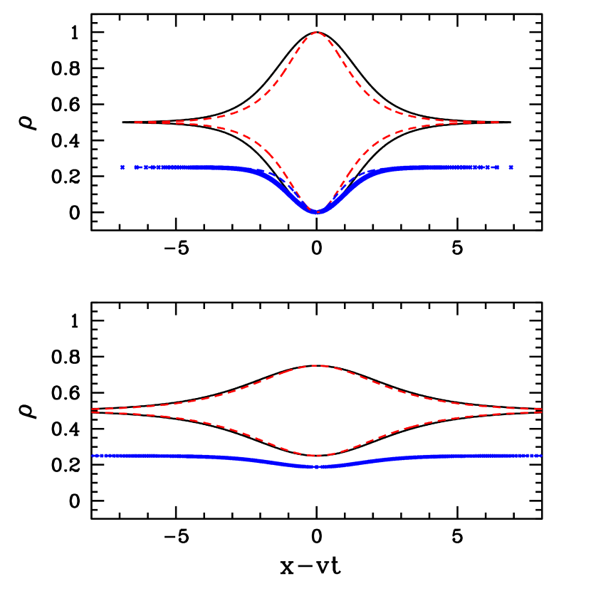
Figure 1: (color online) Comparison of numerical (solid line: black) and analytical (dashed line: red) solitary wave solutions, for $\rho_{0}=0.5$. The upper and lower panels correspond to $\bar{v}=0,\gamma=1$ and $\bar{v}=0.87,\gamma=0.5$, respectively. The plots with crosses (blue) show the corresponding condensate density $\rho^{c}$.

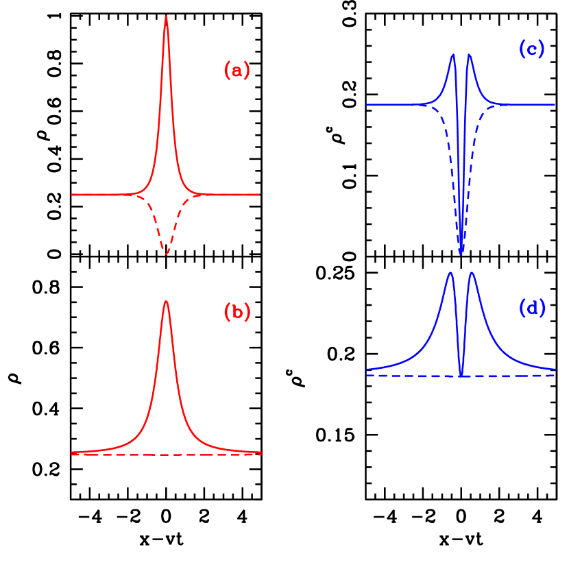
Figure 2: (color online) Solitary wave for $\rho_{0}=0.25$ for total particle density (a,b) and condensate density (c,d), for $\bar{v}=0$ (a,c) and $\bar{v}=1$ (b,d). Solid (dotted) plots correspond to $f^{+}$ ($f^{-}$) solitons.

$$i\hbar\dot{\eta}=-\frac{\hbar^{2}}{2m}\delta\,\,\,\nabla^{2}\eta+\frac{V_{e}}{2}\eta\,\,\,\nabla^{2}\delta+\frac{1}{2}U_{e}(1-\delta)\eta-\mu\eta,\\$$ (6)

$$\dot{\delta}=\frac{\hbar}{2m}\nabla\cdot[(1-\delta^{2})\nabla\phi],$$ (7)

where $ta^{2}=\hbar^{2}/(2m)$ and $V_{e}=Va^{2}$.

In the small-$\eta$ limit where we neglect terms involving $|\eta|^{2n}\eta$ ($n>1$), and retain only linear terms involving the derivatives of $\eta$, both the order parameter equation (6) and the continuity equation (7) reduce to the GPE form, with an effective mean field interaction equal to $U_{e}$. In the above equations, if we set $(1-\delta)=2\rho$ and use Eq. (4), we can show that for $\rho({\bf r})<\frac{1}{2}$, the GPE limit is obtained when $\rho^{c}\approx\rho$, i.e., the order parameter corresponds to the condensate of particles, while for $\rho({\bf r})>\frac{1}{2}$, the GPE is satisfied by the order parameter for the condensate of holes, namely $\eta^{*}$, with $\rho^{c}\approx\rho^{h}$.

The Bogoliubov spectrum associated with the small amplitude modes of the HCB system is similar to the GPEradha1 case and determines the Bogoliubov sound velocity $v_{s}=(U_{e}\rho^{c}/m)^{1/2}$. However, as we discuss below, for the propagation of nonlinear localized modes, true GPE-type transport emerges only near half-filling and the crossover to non-GPE dynamics is controlled by the particle-hole imbalance.

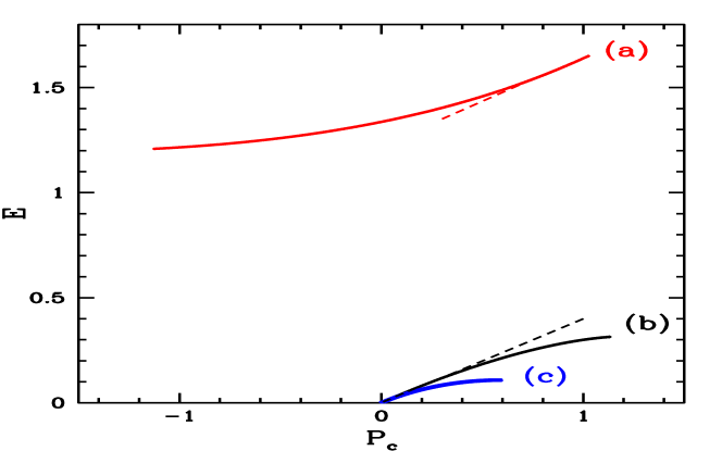
Figure 3: (color online) Energy vs canonical momentum for $\rho_{0}=0.25$ for nn interaction $V=0$. Branches (a) and (b) correspond to the persistent soliton and the dark soliton, respectively. Curve (c) gives the corresponding dispersion for the GPE soliton with $\rho=\rho^{c}_{0}$. The dashed tangents on the two branches demonstrate linear dispersion, with identical slopes.

We now investigate unidirectional soliton propagation in the HCB system, described by Eqs. (6) and (7). To this end, we look for traveling wave solutions for $\rho$ with velocity $v$, of the form $\rho(z)=\rho_{0}+f(z)$, where $z=(x-vt)/a$ and $\rho_{0}$ denotes a uniform background density. The corresponding background particle-hole imbalance is $\delta_{0}=(1-2\rho_{0})$. The function $f(z)$ is then found to satisfy the nonlinear equation

$$4\left(\frac{df}{d\bar{z}}\right)^{2}\left[1-\zeta^{2}\frac{f(f-\delta_{0})}{\rho_{0}^{c}}\right]=f^{2}\left[\gamma^{2}-\frac{f(f-\delta_{0})}{\rho_{0}^{c}}\right],$$ (8)

where $\gamma^{2}=1-\bar{v}^{2}$ with $\bar{v}=v/v_{s}$. Further, $\bar{z}=\zeta z$ and $\zeta=\Lambda/\sqrt{1-\Lambda^{2}}$, where the microscopic parameter $\Lambda=v_{s}\,ma/\hbar$ is the Bogoliubov speed of sound $v_{s}$ measured in units of the zero-point velocity $\hbar/ma$.

Equation (8) is satisfied by an elliptic integral. In the special case where the bracketed term on the left-hand side is approximated by unity, there are two soliton solutions $f^{\pm}$ of the formradha

$$f^{\pm}=\frac{2\gamma^{2}\rho^{c}_{0}}{\pm\sqrt{\delta_{0}^{2}+4\gamma^{2}\rho^{c}_{0}}\,\,\cosh\,(z/\Gamma)-\delta_{0}}.$$ (9)

Here, $\Gamma=2\zeta\gamma$ is the width of the soliton. These two special solutions are emblematic of the general solution to Eq. (8). We have numerically integrated Eq. (8) to find $f(z)$, and compared it with the analytical solution (9). We find close agreement between the numerical and analytical solutions for all values of $v$ and $\rho_{0}$. This happens because the neglected terms become irrelevant for small $f$ and also when $\frac{df}{dz}=0$, the condition which determines almost all the contributions to the localized modes. Fig. 1 with $\rho_{0}=1/2$ shows the case when the agreement is at its worst. Away from half-filling, the numerical and analytic solutions are very close.

The solutions (9) are valid provided $U_{e}>0$ (or $t>V$), because the functions $f^{\pm}$ are unbounded for negative $U_{e}$. We point out that the interaction $V$ simply scales the width of the soliton, without altering its profile. This leads to an interesting possibility that the existence of the soliton and its overall profile may remain unaffected by certain long range interactions.Baiz

The distinction between the twin solitons, which encode particle-hole duality as $f^{+}(z,\rho_{0})=f^{-}(z,\rho_{0}^{h})$, can be elucidated by computing the momentum $P^{\pm}=m\int J^{\pm}dx$. Here $J=(\hbar/m)\rho_{c}\nabla\phi$ (see Eq. (7)) is the condensate current, which is obtained using the equationradha $d\phi/dz=vma\,(\rho^{\pm}~{}-~{}\rho_{0})/\hbar\rho_{c}$. We get

$$P^{\pm}=\pm(mv)\frac{\sqrt{\rho_{c}^{0}}}{2\zeta}\tan^{-1}\sqrt{\frac{(\delta_{0}^{2}+2\rho_{c}^{0}\gamma^{2})^{1/2}\pm\delta_{0}}{(\delta_{0}^{2}+2\rho_{c}^{0}\gamma^{2})^{1/2}\mp\delta_{0}}}\,.$$ (10)

For small $v$, $P^{+}$ corresponds to the momentum of a particle of positive mass while $P^{-}$ corresponds to the momentum of a hole, as the effective mass is negative. This justifies associating $f^{+}$ [respectively, $f^{-}$] as the solitary wave with particles [holes]. Further, $(P^{+}-P^{-})/mv=\pi\zeta/\sqrt{\rho^{c}_{0}}$, which is suggestive of a conservation principle.

Particle-hole imbalance appears to be a key factor in determining the characteristics of the solitary waves. As seen in Fig.  1, when the number of particles is equal to the number of holes, the two solutions for the particle density $\rho(z)$ are dark and anti-darkanti solitons ( bright solitons on a pedestal) which are mirror images of each other. In the corresponding condensate density $\rho^{c}(z)$, the solutions are indistinguishable, resulting in a single GPE-like soliton, that flattens out at the sound velocity. In fact, within the approximations discussed above, Eq. (8) expressed in terms of the condensate density $\rho_{c}(z)$ is identical to a GPE with healing length $\xi$ renormalized to $\frac{1}{2}\xi\sqrt{1-\Lambda^{2}}$. In other words, when the background consists of equal numbers of particles and holes, the soliton solution for the condensate density of the HCB is like the usual soliton of the GPE, but with a renormalized healing length.

When the number of particles differs from the number of holes, the condensate soliton corresponding to the solution $f^{-}$ is dark and flattens out at the sound velocity. However, the condensate soliton corresponding to the solution $f^{+}$ brightens the condensate profile, as shown in Fig. 2. As $v$ increases, the spatial extent of the disturbance above the background increases, and the solitary wave $\rho^{c}(z)$ becomes completely bright at the speed of sound. More important, this soliton does not flatten out but persists even at the sound velocity. The survival or persistence of the soliton of this sector is evident from the limiting functional formsky of $f^{+}$ as $\bar{v}\rightarrow 1$. We find $\rho^{+}\rightarrow\rho_{0}+\delta_{0}/(1+Cz^{2})$, where $C=4\zeta^{2}\delta_{0}/\rho^{c}_{0}$ and hence the width of the soliton becomes independent of its speed of propagation. It should be noted that as $\rho_{0}\rightarrow 0$, the solutions approach a definite limit with $C$ equals to $8U_{e}$ in units of zero-point energy $(\hbar/a)^{2}/m$. In other words, the anti-dark solitons become bright solitons, reminiscent of the bright solitons discussed in systems with attractive dipole-dipole interaction.Baiz

Another distinctive feature of the persistent soliton is that it is transformed into a periodic wave train when its velocity exceeds the sound velocity. Indeed, inspection of Eq. (9) shows that at supersonic speeds, when $\gamma$ becomes imaginary, the soliton is transformed to a spatially periodic wave that exists for velocities $v_{s}<v<v_{s}/(1-\delta_{0}^{2})$.

Finally, we compute the energy-momentum relationship of the solitons by integrating the equation $dE/dP_{c}=v$ to obtain the canonical momentum $P_{c}$, where $E$ is the energyPitabook . The three plots in Fig.  3 show the dispersion relations for the $f^{+}$ and $f^{-}$ solitons, and the corresponding GPE solitonBC . Each plot shows linear dispersion at one end of the spectrum (at the momentum corresponding to $v=v_{s}$), and saturation at the other end (at the momentum corresponding to $v=0$). The dark soliton has a linear dispersion near $E=0,P_{c}=0$), with the slope given by $v_{s}$, and it saturates to zero slope near the maximum value of the momentum. (The GPE soliton, with $\rho=\rho_{0}^{c}$, has a similar behavior). The persistent soliton exhibits linear dispersion with the same slope $v_{s}$ near the maximum value of the momentum. Comparing this with the exact bosonic low-lying excitation spectrum for the HCB gas discussed by Lieb Lieb , we note that both soliton branches with bounded momentum intervals, mimic the main characteristics of his type II excitation spectrum, being linear at one end and saturating at the other. However, it should be noted that in the present context, it is the lower branch that can be designated as a type II ‘hole’ state. The higher energy upper branch associated with the persistent soliton is in fact a type II ‘particle’ state. This is different from Lieb’s classification, where ‘particle’ states were always type I with unbounded momentum.

In summary, we have explored solitary wave propagation in a degenerate HCB gas, and have found novel features that are not present in the conventional Gross-Pitaevskii equation, as well as some others that are. In a lattice system, this cross-over occurs at half-filling, which corresponds to equal numbers of particles and holes in the HCB system. At exact half-filling, we obtain GPE-like dark solitary waves. Away from half-filling, we find both dark and anti-dark solitary waves including a persistent variety which propagates with a non-vanishing amplitude right up to the speed of the sound. The forms of these solutions at $t=0$ represent two initial types of disturbance profiles that could evolve into these solitons in realistic quasi-one-dimensional systems. These aspects could be further explored in numerical simulation in first-principle quantum many-body calculations and may find experimental realization in a highly anisotropic cigar shaped trap. We hope that our results will also provide further stimulus to the study of solitons in quantum many-body systems.

References

- (1) M. Girardeau, J. Math. Phys. 1, 516 (1960).
- (2) F. Herbet et al., Phys. Rev. B 65, 014513 (2002).
- (3) M. D. Girardeau and E. M. Wright, Phys. Rev. Lett. 84, 5691 (2000); Phys. Rev. A 77, 043612 (2008).
- (4) T. Matsubara and H. Matsuda, Prog. Theor. Phys. 16, 569 (1956).
- (5) S. Burger et al., Phys. Rev. Lett. 83, 5198 (1999); J. Denschlag et al., Science 287, 97 (2000)
- (6) E. Kolomeisky, T. J. Newman, J. Straley, and X. Qi, Phys. Rev. Lett. 85, 1146 (2000).
- (7) G. L. Alfimov et al., Phys Rev. A, 75, 023624 (2007).
- (8) B. B. Baizakov et al. J. Phys. B: At. Mol. Opt. Phys., 42 (2009) 175302; G. Gligoric et al, Phys Rev A, 78 063615, (2008).
- (9) K. V. Krutitsky et al., arXiv: 0907.0625 (2009); V. Mishmash et al., arXiv: 0906.4949 (2009).
- (10) See for example, S.Sachdev Quantum Phase Transitions, (Cambridge University Press, Cambridge, 1999).
- (11) R. Balakrishnan, R. Sridhar, and R. Vasudevan, Phys. Rev. B 39 174, (1989).
- (12) K. Mitra, C. J. Williams, and C.A.R. Sa de Melo, Phys. Rev. A, 77, 033607 (2008).
- (13) L. Pitaevskii and S. Stringari, Bose-Einstein Condensation (Oxford University Press, Oxford, 2003).
- (14) R. Balakrishnan, Phys. Rev. B 42, 6153 (1990).
- (15) Y. S. Kivshar and V. V. Afanasjev, Phys. Rev. A 44, R1446 (1991).
- (16) This solution is reminiscent of the skyrmion in 2D: with , these solitons correspond to configurations with up spins at and down spins at .
- (17) The integration is done using the boundary condition when for the soliton. For the soliton, we use the condition , because the twin solitons have equal and opposite phase jumps at .
- (18) E. H. Lieb, Phys Rev, 130 (1963), 1616.