Black Holes in the Dilatonic Einstein-Gauss-Bonnet Theory in Various Dimensions IV
– Topological Black Holes with and without Cosmological Term –

Abstract

We study black hole solutions in the Einstein gravity with Gauss-Bonnet term, the dilaton and a positive “cosmological constant” in various dimensions. Physically meaningful black holes with a positive cosmological term are obtained only for those in static spacetime with $(D-2)$-dimensional hyperbolic space of negative curvature and $D\geq 5$. We construct such black hole solutions of various masses numerically in $D=5,6$ and 10 dimensional spacetime and discuss their properties. In spite of the positive cosmological constant the spacetime approach anti-de Sitter spacetime asymptotically. The black hole solutions exist for a certain range of the horizon radius, i.e., there are lower and upper bounds for the size of black holes. We also argue that it is quite plausible that there is no black hole solution for hyperbolic space in the case of no cosmological constant.

1 Introduction

This is the fourth and final of a series of our papers in which we study the static black hole solutions in dilatonic Einstein-Gauss-Bonnet theory in higher dimensions. [1, 2, 3]

There have been many works on black hole solutions in dilatonic gravity since the work in Refs. GM and GHS. Because there are higher-order quantum corrections and dilaton in string theories, [6] it is important to study how these modify the results. Several works have studied the effects of higher order terms but only in four dimensions, [7, 8, 9, 10, 11] or considered theories without dilaton. [12, 13, 14] Motivated by this situation, we started our study of black hole solutions and their properties in the theory with the higher order corrections and dilaton in dimensions higher than or equal to four. The simplest higher order correction is the Gauss-Bonnet (GB) term, which may appear in heterotic string theories.

In our first paper in this series, [1] we have studied black hole solutions with the GB correction term and dilaton without the cosmological term for asymptotically flat solutions in various dimensions from 4 to 10 with $(D-2)$-dimensional hypersurface with curvature signature $k=+1$. We tried to find topological black holes for $k=-1$, but it turned out that there is no solution without the cosmological term. We have then presented our results on black hole solutions with a negative cosmological term with $(D-2)$-dimensional hypersurface with $k=0,\pm 1$ in the second and third papers. [2, 3] In the context of string theories, it is very interesting to examine asymptotically non-flat black hole solutions with possible applications to AdS/CFT and dS/CFT correspondence in mind. [15] Discussions of the origin of such cosmological terms are given in Refs. AGMV,POL. In our systematic study of these static black hole solutions, those cases with the positive cosmological term and those for hyperbolic space without the cosmological term have not been studied. In this paper, we continue our study of the black holes for these remaining cases and complete our study. Cosmological solutions in such a system are considered in Ref. BGO.

This paper is organized as follows. In § 2, we first summarize our action with the GB and the cosmological terms, and give basic equations to solve. We then discuss symmetry properties of the theory which will be useful in our following analysis. In § 3, boundary conditions at the horizon and asymptotic behaviors are discussed for our solutions. In § 4, we discuss asymptotic expansions and allowed parameter regions for the existence of black holes in the case with the positive cosmological term. We show that there is no allowed parameter region for $D=4$ and hence there is no black hole solution. We then argue that there is no asymptotically de Sitter (dS) solutions due to the presence of a non-normalizable mode in higher dimensions. We find, however, that there are asymptotically anti-de Sitter (AdS) solutions for appropriate range of parameters even though we have the positive cosmological term. In § 5, we present these solutions in $D=5,6$ and 10 with a positive cosmological term for $k=-1$. Though we do not present explicit solutions for other $D=7,8$ and 9, the properties are similar [1] and we expect that there are similar solutions. In § 6, we show that there is no black hole solution for $k=0$. In § 7, we argue that there is no physically meaningful black hole solution for $k=1$ for some parameter range in our action in general unless miraculous cancellation of the growing mode of the dilaton happens, although there does exist an exact regular dS solution with constant dilaton. For other range of the parameters, there may be regular (not black hole) solutions, which will be studied elsewhere. These solutions and discussions are given for particular choices of the parameters in our theory, but we expect that the qualitative behaviors do not change for other choices.

In § 8, we discuss topological black holes with $k=-1$ for zero cosmological term, and show that there is no black hole solution in $D=4$. In higher dimensions, we find that there is a narrow range of the value of the dilaton at the horizon where solutions may exist. We have not found, however, black hole solutions even for this range, and most probably there is no black hole solution at least for the dilaton coupling $\gamma=\frac{1}{2}$, though we do not have rigorous proof.

§ 9 is devoted to conclusions and discussions. In particular, we summarize our main results obtained in this series of papers.

2 Dilatonic Einstein-Gauss-Bonnet theory

2.1 Action and basic equations

We consider the following low-energy effective action for a heterotic string

$$S=\frac{1}{2\kappa_{D}^{2}}\int d^{D}x\sqrt{-g}\left[R-\frac{1}{2}(\partial_{\mu}\phi)^{2}+\alpha_{2}e^{-\gamma\phi}R^{2}_{\rm GB}-\Lambda e^{\lambda\phi}\right],$$ (1)

where $\kappa_{D}^{2}$ is a $D$-dimensional gravitational constant, $\phi$ is a dilaton field, $\alpha_{2}=\alpha^{\prime}/8$ is a numerical coefficient given in terms of the Regge slope parameter $\alpha^{\prime}$, and $R^{2}_{\rm GB}=R_{\mu\nu\rho\sigma}R^{\mu\nu\rho\sigma}-4R_{\mu\nu}R^{\mu\nu}+R^{2}$ is the GB correction. For the moment, we leave the coupling constant of dilaton $\gamma$ arbitrary, while the ten-dimensional critical string theory predicts $\gamma=1/2$ which is the value we choose in our numerical analysis. We have also included the positive cosmological constant $\Lambda=(D-1)_{2}/\ell^{2}$ with possible dilaton coupling $\lambda$. If this is the only potential of the dilaton field, there is no stationary point and the dilaton cannot have a stable asymptotic value. However, for asymptotically (A)dS solutions, the GB term can be regarded as an additional “potential” in the asymptotic region, and we will see that it is possible to have the solutions where the dilaton takes finite constant value at infinity. There may be several possible sources of “cosmological terms” with different dilaton couplings, so we leave $\lambda$ arbitrary and specify it in the numerical analysis.

We parametrize the metric as

$$ds_{D}^{2}=-Be^{-2\delta}dt^{2}+B^{-1}dr^{2}+r^{2}h_{ij}dx^{i}dx^{j},$$ (2)

where $h_{ij}dx^{i}dx^{j}$ represents the line element of a $(D-2)$-dimensional hypersurface with constant curvature $(D-2)(D-3)k$ and volume $\Sigma_{k}$ for $k=\pm 1,0$.

The metric function $B=B(r)$ and the lapse function $\delta=\delta(r)$ depend only on the radial coordinate $r$. The field equations are [2, 3]

$$\bigl{[}(k-B)\tilde{r}^{D-3}\bigr{]}^{\prime}\frac{D-2}{\tilde{r}^{D-4}}h-\frac{1}{2}B\tilde{r}^{2}{\phi^{\prime}}^{2}-(D-1)_{4}\,e^{-\gamma\phi}\frac{(k-B)^{2}}{\tilde{r}^{2}}$$

$$\hskip 28.45274pt+4(D-2)_{3}\,\gamma e^{-\gamma\phi}B(k-B)(\phi^{\prime\prime}-\gamma{\phi^{\prime}}^{2})$$

$$\hskip 28.45274pt+2(D-2)_{3}\,\gamma e^{-\gamma\phi}\phi^{\prime}\frac{(k-B)[(D-3)k-(D-1)B]}{\tilde{r}}-\tilde{r}^{2}\tilde{\Lambda}e^{\lambda\phi}=0\,,$$ (3)

$$\delta^{\prime}(D-2)\tilde{r}h+\frac{1}{2}\tilde{r}^{2}{\phi^{\prime}}^{2}-2(D-2)_{3}\,\gamma e^{-\gamma\phi}(k-B)(\phi^{\prime\prime}-\gamma{\phi^{\prime}}^{2})=0\,,$$ (4)

$$(e^{-\delta}\tilde{r}^{D-2}B\phi^{\prime})^{\prime}=\gamma(D-2)_{3}e^{-\gamma\phi-\delta}\tilde{r}^{D-4}\Big{[}(D-4)_{5}\frac{(k-B)^{2}}{\tilde{r}^{2}}+2(B^{\prime}-2\delta^{\prime}B)B^{\prime}$$

$$\hskip 28.45274pt-4(k-B)BU(r)-4\frac{D-4}{\tilde{r}}(B^{\prime}-\delta^{\prime}B)(k-B)\Big{]}+e^{-\delta}\tilde{r}^{D-2}\lambda\tilde{\Lambda}e^{\lambda\phi},$$ (5)

where we have defined the dimensionless variables: $\tilde{r}\equiv r/\sqrt{\alpha_{2}}$, $\tilde{\Lambda}\equiv\alpha_{2}\Lambda$, and the primes in the field equations denote the derivatives with respect to $\tilde{r}$. Namely we measure our length in the unit of $\sqrt{\alpha_{2}}$. We have defined

$$(D-m)_{n} \equiv (D-m)(D-m-1)(D-m-2)\cdots(D-n),$$

$$h \equiv 1+2(D-3)e^{-\gamma\phi}\Big{[}(D-4)\frac{k-B}{\tilde{r}^{2}}+\gamma\phi^{\prime}\frac{3B-k}{\tilde{r}}\Big{]},$$ (6)

$$\tilde{h} \equiv 1+2(D-3)e^{-\gamma\phi}\Big{[}(D-4)\frac{k-B}{\tilde{r}^{2}}+\gamma\phi^{\prime}\frac{2B}{\tilde{r}}\Big{]},$$ (7)

$$U(r) \equiv (2\tilde{h})^{-1}\Bigg{[}(D-3)_{4}\frac{k-B}{\tilde{r}^{2}B}-2\frac{D-3}{\tilde{r}}\Big{(}\frac{B^{\prime}}{B}-\delta^{\prime}\Big{)}-\frac{1}{2}\phi^{\prime 2}$$ (8)

$$+(D-3)e^{-\gamma\phi}\Bigg{\{}(D-4)_{6}\frac{(k-B)^{2}}{\tilde{r}^{4}B}-4(D-4)_{5}\frac{k-B}{\tilde{r}^{3}}\Big{(}\frac{B^{\prime}}{B}-\delta^{\prime}-\gamma\phi^{\prime}\Big{)}$$

$$-4(D-4)\gamma\frac{k-B}{\tilde{r}^{2}}\Big{(}\gamma\phi^{\prime 2}+\frac{D-2}{\tilde{r}}\phi^{\prime}-\Phi\Big{)}+8\frac{\gamma\phi^{\prime}}{\tilde{r}}\biggl{[}\Big{(}\frac{B^{\prime}}{2}-\delta^{\prime}B\Big{)}\Big{(}\gamma\phi^{\prime}-\delta^{\prime}+\frac{2}{\tilde{r}}\Big{)}$$

$$-\frac{D-4}{2\tilde{r}}B^{\prime}\biggr{]}+4(D-4)\Big{(}\frac{B^{\prime}}{2B}-\delta^{\prime}\Big{)}\frac{B^{\prime}}{\tilde{r}^{2}}-\frac{4\gamma}{\tilde{r}}\Phi(B^{\prime}-2\delta^{\prime}B)\Bigg{\}}-\frac{1}{B}\tilde{\Lambda}e^{\lambda\phi}\Biggr{]},$$

$$\Phi \equiv \phi^{\prime\prime}+\Big{(}\frac{B^{\prime}}{B}-\delta^{\prime}+\frac{D-2}{\tilde{r}}\Big{)}\phi^{\prime}.$$ (9)

2.2 Symmetry and scaling

It is useful to consider several scaling symmetries of our field equations (or our model). Firstly the field equations are invariant under the transformation:

$$\gamma\to-\gamma,~{}~{}\lambda\to-\lambda,~{}~{}\phi\to-\phi\,.$$ (10)

By this symmetry, we can restrict the parameter range of $\gamma$ to $\gamma\geq 0$.

The field equations (3) – (5) have a shift symmetry:

$$\phi\to\phi-\phi_{\ast},~{}~{}\tilde{\Lambda}\to e^{(\lambda-\gamma)\phi_{\ast}}\tilde{\Lambda},~{}~{}r\to e^{-\gamma\phi_{\ast}/2}r.$$ (11)

where $\phi_{\ast}$ is an arbitrary constant. This changes the magnitude of the cosmological constant. Hence this may be used to generate solutions for different cosmological constants, given a solution for some cosmological constant and $\tilde{r}_{H}$. Details will be discussed in § 5.

The third one is the shift symmetry under

$$\delta\to\delta-\delta_{\ast},~{}~{}t\to e^{-\delta_{\ast}}t,$$ (12)

with an arbitrary constant $\delta_{\ast}$, which may be used to shift the asymptotic value of $\delta$ to zero.

For $k=0$, the field equations (3)–(5) are invariant under the scaling transformation

$$B\to a^{2}B,~{}~{}\tilde{r}\to a\tilde{r},$$ (13)

with an arbitrary constant $a$. If a black hole solution with the horizon radius $\tilde{r}_{H}$ is obtained, we can generate solutions with different horizon radii but the same $\tilde{\Lambda}$ by this scaling transformation.

The model (1) has several parameters of the theory such as $D$, $\alpha_{2}$, $\Lambda$, $\gamma$, and $\lambda$. The black hole solutions have also physical parameters such as the horizon radius $\tilde{r}_{H}$ and the value of $\delta$ at infinity. However owing to the above symmetries (including the scaling by $\alpha_{2}$), we can reduce the number of the parameters and are left only with $D$, $\gamma\geq 0$, $\lambda$, and $\tilde{r}_{H}$.

3 Boundary conditions

In this paper, we study solutions with spherical ($k=+1$), planar ($k=0$) and hyperbolic ($k=-1$) symmetries with a positive cosmological constant $\tilde{\Lambda}>0$ except for § 8 where we study solutions with $k=-1$ and $\Lambda=0$. In this section, we discuss the boundary conditions and asymptotic behaviors for these solutions.

3.1 Regular horizon

Let us first examine the boundary conditions of the black hole spacetime. We impose the following boundary conditions for the metric functions:

1. The existence of a regular black hole horizon at $\tilde{r}=\tilde{r}_{BH}$:

   $$B(\tilde{r}_{BH})=0,~{}~{}B^{\prime}(\tilde{r}_{BH})>0,~{}~{}|\delta(\tilde{r}_{BH})|<\infty,~{}~{}|\phi(\tilde{r}_{BH})|<\infty\,.$$ (14)

2. The absence of singularities outside the black hole event horizon ($\tilde{r}>\tilde{r}_{BH}$).

Since our model (1) has the positive cosmological constant, there may be cosmological horizon at $\tilde{r}=\tilde{r}_{CH}>\tilde{r}_{BH}$ with the second condition in Eq. (14) replaced by $B^{\prime}(\tilde{r}_{CH})<0$. Here and in what follows, the values of various quantities at the black hole and the cosmological horizons are denoted with subscripts $BH$ and $CH$, respectively. When we refer to both horizons, we simply use the subscript $H$.

When $B^{\prime}(\tilde{r}_{BH})=0$, the horizon is degenerate, and the spacetime can be the extreme black hole if $B^{\prime\prime}(\tilde{r}_{BH})>0$.

At the horizon, it follows from Eqs. (3), (6), and (7) that

$$B_{H}=0,$$

$$h_{H}=1+(D-4-\gamma\phi_{H}^{\prime}\tilde{r}_{H})C,$$

$$\tilde{h}_{H}=1+(D-4)C,$$

$$B_{H}^{\prime}h_{H}=\frac{(D-3)k}{\tilde{r}_{H}}+\frac{(D-4)_{5}kC}{2}-\frac{\tilde{r}_{H}L}{D-2},$$ (15)

where we have defined

$$C\equiv\frac{2(D-3)ke^{-\gamma\phi_{H}}}{\tilde{r}_{H}^{2}},~{}~{}L\equiv e^{\lambda\phi_{H}}\tilde{\Lambda}.$$ (16)

Using these in Eq. (5) gives

$$2C\gamma\Big{[}-2L\tilde{r}_{H}^{2}\Big{\{}1+C\big{[}D-4-(D-2)\gamma\lambda\big{]}+(D-2)C^{2}\gamma\big{[}(D-6)\gamma-(D-4)\lambda\big{]}\Big{\}}$$

$$\hskip 28.45274pt+(D-2)k\Big{\{}2(D-3)+(D-4)(3D-11)C$$

$$\hskip 42.67912pt+(D-4)C^{2}\big{[}(D-2)(3D-11)\gamma^{2}+(D-4)_{5}\big{]}+2(D-2)_{5}C^{3}\gamma^{2}\Big{\}}\Big{]}\tilde{r}_{H}^{2}\phi_{H}^{\prime 2}$$

$$+2\Big{[}4C^{2}\gamma^{2}L^{2}\tilde{r}_{H}^{4}+2L\tilde{r}_{H}^{2}\Big{\{}1+2C\big{[}D-4-(D-2)\gamma\lambda\big{]}$$

$$\hskip 56.9055pt-C^{2}\big{[}2(D-2)(2D-5)\gamma^{2}+4(D-2)(D-4)\gamma\lambda-(D-4)^{2}\big{]}$$

$$\hskip 56.9055pt-2(D-2)(D-4)C^{3}\gamma\big{[}(D-2)\gamma+(D-4)\lambda\big{]}\Big{\}}$$

$$\hskip 28.45274pt+(D-2)k\Big{\{}(D-1)_{2}(D-4)C^{2}\gamma^{2}\big{[}2+2kC-(D-4)_{5}C^{2}\big{]}$$

$$\hskip 85.35826pt-\big{[}1+(D-4)C\big{]}^{2}\big{[}2(D-3)+(D-4)_{5}C\big{]}\Big{\}}\Big{]}\tilde{r}_{H}\phi_{H}^{\prime}$$

$$+4\frac{C}{k}\gamma L^{2}\tilde{r}_{H}^{4}+4(D-2)L\tilde{r}_{H}^{2}\Big{\{}\lambda\big{[}1+(D-4)C\big{]}^{3}$$

$$\hskip 85.35826pt+C\gamma\big{[}D(D-4)^{2}C^{2}+(D-4)(D+1)C-(D-2)\big{]}\Big{\}}$$

$$\hskip 14.22636pt+(D-1)_{2}(D-2)kC\gamma\Big{\{}2(D-2)-4(D-4)C-(D-4)^{2}(D+1)C^{2}\Big{\}}=0,$$ (17)

This equation gives the value of the derivative of the dilaton field at a horizon for given $\tilde{r}_{H}$ and $\phi_{H}$.

3.2 Asymptotic behavior at infinity and cosmological horizon

If the solution can be continued outside the cosmological horizon, we impose the condition that the leading term of the metric function $B$ comes from dS radius at infinity. Since the curvatures do not vanish for asymptotically non-flat case in general and the GB term contributes in the asymptotic region, the spacetime can approach non-dS spacetime as we will see later. So we impose the following condition:

1. “Appropriate” asymptotic behavior at infinity ($\tilde{r}\to\infty$):

   $$B\sim\tilde{b}_{2}\tilde{r}^{2}+k-\frac{2\tilde{M}}{\tilde{r}^{\mu}},~{}~{}~{}\delta(r)\sim\delta_{0}+\frac{\delta_{1}}{\tilde{r}^{\sigma}},~{}~{}\phi\sim\phi_{0}+\frac{\phi_{1}}{\tilde{r}^{\nu}}\,,$$ (18)

   with finite constants $\tilde{b}_{2}$, $\tilde{M}$, $\delta_{0}$, $\delta_{1}$, $\phi_{0}$, $\phi_{1}$ and positive constant $\mu$, $\sigma$, $\nu$. Depending on the sign of the constant $\tilde{b}_{2}$, the spacetime has different asymptotics, i.e. dS for $\tilde{b}_{2}<0$, flat for $\tilde{b}_{2}=0$, and AdS for $\tilde{b}_{2}>0$.

3.3 Behaviors of dilaton between black hole and cosmological horizons

The equation of the dilaton field (5) is rewritten as

$$e^{-\delta}B\phi^{\prime\prime}+\frac{1}{\tilde{r}^{D-2}}\bigl{(}\tilde{r}^{D-2}e^{-\delta}B\bigr{)}^{\prime}\phi^{\prime}=e^{-\delta}\bigl{(}\gamma e^{-\gamma\phi}\tilde{R}_{GB}^{2}+\lambda\tilde{\Lambda}e^{\lambda\phi}\bigr{)}.$$ (19)

where

$$\tilde{R}_{GB}^{2}=\frac{(D-2)_{3}}{\tilde{r}^{2}}\biggl{[}(D-4)_{5}\frac{(k-B)^{2}}{\tilde{r}^{2}}+2(B^{\prime}-2\delta^{\prime}B)B^{\prime}$$

$$\hskip 28.45274pt-4(k-B)\Bigl{(}\frac{1}{2}B^{\prime\prime}-B\delta^{\prime\prime}-\frac{3}{2}B^{\prime}\delta^{\prime}+B\delta^{\prime 2}\Bigr{)}-\frac{4(D-4)}{\tilde{r}}(k-B)(B^{\prime}-\delta^{\prime}B)\biggr{]}.$$ (20)

In the Einstein theory ($\tilde{R}_{GB}^{2}=0$), since $B=0$ on the horizons, $\phi^{\prime}_{H}$ is expressed by $\phi_{H}$ as

$$\phi_{H}^{\prime}=\frac{1}{B_{H}^{\prime}}\lambda\tilde{\Lambda}e^{\lambda\phi_{H}}.$$ (21)

We assume $\lambda<0$ from the consideration of the asymptotic condition (18) presented in the next section. This implies that $\phi$ decreases around the black hole because $B^{\prime}$ is positive near the black hole horizon, i.e., the right hand side (r.h.s.) of Eq. (21) is negative. Similarly it is locally increasing function around the cosmological horizon because $B_{CH}^{\prime}<0$. These mean that the dilaton field has to have a local minimum in $\tilde{r}_{BH}<\tilde{r}<\tilde{r}_{CH}$. On the other hand, at the extremum of the dilaton field ($\phi^{\prime}=0$), Eq. (19) gives

$$B\phi^{\prime\prime}=\lambda\tilde{\Lambda}e^{\lambda\phi}.$$ (22)

It then follows that $\phi^{\prime\prime}<0$ since $B>0$ for $\tilde{r}_{BH}<\tilde{r}<\tilde{r}_{CH}$. Hence the dilaton field does not have the local minimum in this region. This contradicts the behaviors around both the horizons. We can thus conclude that there is no static black hole solution with $k=\pm 1,\>0$ in the Einstein-dilaton case.

In the GB case, however, the situation is different. The r.h.s. of Eq. (19) can take both signs at the horizons and at the extremum of the dilaton field. Hence Eqs. (3)-(5) may have the consistent solutions between $\tilde{r}_{BH}$ and $\tilde{r}_{CH}$ which satisfy the condition at each horizon. It should be noted here that $\phi$ and $\phi^{\prime}$ cannot be free but are related with each other by the condition (17) at the cosmological horizon. In order to satisfy this condition, we have to tune the value of $\phi_{BH}$ as a shooting parameter for each $\tilde{r}_{BH}$. This will have important consequence in the subsequent discussions.

4 Asymptotic expansions and allowed parameter regions

4.1 Asymptotic expansion

Substituting Eqs. (18) into the field equations (3) and (5), one finds the conditions that the leading terms ($\tilde{r}^{2}$ and constant terms in each equation) should satisfy are given by

$$(D)_{3}\gamma\;e^{-\gamma\phi_{0}}\tilde{b}_{2}^{~{}2}+\lambda\tilde{\Lambda}e^{\lambda\phi_{0}}=0\,,$$ (23)

$$(D-1)_{4}\;e^{-\gamma\phi_{0}}\tilde{b}_{2}^{~{}2}-(D-1)_{2}\tilde{b}_{2}-\tilde{\Lambda}e^{\lambda\phi_{0}}=0\,,$$ (24)

which determine $\tilde{b}_{2}$ and $\phi_{0}$, while $\delta_{0}$ can be arbitrary because only its derivative appears in our field equations. Since $\tilde{\Lambda}$ and $\gamma$ are positive, $\lambda$ should be negative by Eq. (23). The positivity of $\tilde{\Lambda}$ means that $\tilde{b}_{2}\neq 0$ by Eq. (24). So there is no solution with asymptotically flat spacetime under our assumptions. We also find that

$$\left\{\begin{array}[]{lcl}\gamma>\dfrac{D-4}{D}|\lambda|&~{}\Longrightarrow{}&\tilde{b}_{2}<0~{}~{}({\rm dS}),\\ \gamma=\dfrac{D-4}{D}|\lambda|&~{}\Longrightarrow{}&\tilde{b}_{2}=0~{}~{}(\mbox{not allowed}),\rule[0.0pt]{0.0pt}{22.76219pt}\\ \gamma<\dfrac{D-4}{D}|\lambda|&~{}\Longrightarrow{}&\tilde{b}_{2}>0~{}~{}({\rm AdS}).\rule[0.0pt]{0.0pt}{22.76219pt}\end{array}\right.$$ (28)

Eqs. (23) and (24) give

$$\tilde{b}_{2}^{~{}2}=\frac{-\lambda\tilde{\Lambda}}{(D)_{3}\gamma}\biggl{[}\frac{D(D-3)}{(D-1)_{2}}\frac{\tilde{\Lambda}\gamma}{(-\lambda)}\biggl{(}1+\frac{(D-4)\lambda}{D\gamma}\biggr{)}^{2}\biggr{]}^{\frac{\gamma+\lambda}{\gamma-\lambda}},$$ (29)

$$e^{\phi_{0}}=\biggl{[}\frac{D(D-3)}{(D-1)_{2}}\frac{\tilde{\Lambda}\gamma}{(-\lambda)}\biggl{(}1+\frac{(D-4)\lambda}{D\gamma}\biggr{)}^{2}\biggr{]}^{\frac{1}{\gamma-\lambda}}.$$ (30)

The candidates of the next leading terms for Eqs. (3)-(5) are respectively given by

$$\bigl{[}\mu-(D-3)\bigr{]}\bigl{[}(D-4)\lambda-D\gamma\bigr{]}\tilde{M}\tilde{r}^{-\mu}-2\gamma\lambda(\nu+1)\bigl{[}\nu-(D-1)\bigr{]}\tilde{b}_{2}\phi_{1}\tilde{r}^{2-\nu}\,,$$ (31)

$$\rule[0.0pt]{0.0pt}{19.91692pt}\bigl{[}(D-4)\lambda-D\gamma\bigr{]}\sigma\delta_{1}\tilde{r}^{-\sigma}+2\lambda\gamma\nu(\nu+1)\phi_{1}\tilde{r}^{-\nu}\,,$$ (32)

$$\rule[0.0pt]{0.0pt}{19.91692pt}4(D-2)\lambda\gamma\sigma(\sigma-D)\tilde{b}_{2}\delta_{1}\tilde{r}^{-\sigma}$$

$$\hskip 28.45274pt+\Bigl{\{}(D)_{2}\lambda\gamma(\lambda+\gamma)+\bigl{[}(D-4)\lambda+D\gamma\bigr{]}\nu\bigl{[}\nu-(D-1)\bigr{]}\Bigr{\}}\tilde{b}_{2}\phi_{1}\tilde{r}^{-\nu}$$

$$\hskip 28.45274pt+4(D-2)\lambda\gamma\bigl{[}\mu-(D-2)\bigr{]}\bigl{[}\mu-(D-3)\bigr{]}\tilde{M}\tilde{r}^{-\mu-2}\,,$$ (33)

which should all vanish. There are two different classes which give consistent expansions. One is $\mu=D-3$ and $\nu,\sigma>D-1$, and we rename the coefficient $\tilde{M}$ as $\tilde{M}_{0}$. The other class is $\mu=\nu-2=\sigma-2$ and

$$\nu=\nu_{\pm}\equiv\frac{D-1}{2}\left[1\pm\sqrt{1-\frac{4(D)_{2}\lambda\gamma(\lambda-\gamma)\bigl{[}(D-4)\lambda+D\gamma\bigr{]}}{(D-1)^{2}\bigl{[}(D-4)^{2}\lambda^{2}-D^{2}\gamma^{2}-8(D-1)_{2}\lambda^{2}\gamma^{2}\bigr{]}}}\;\right].$$ (34)

The asymptotic forms of the fields are then

$$\phi\sim\phi_{0}+\frac{\phi_{+}}{\tilde{r}^{\nu_{+}}}+\cdots\,,$$

$$B\sim\tilde{b}_{2}\tilde{r}^{2}+k-\frac{2\tilde{M}_{+}}{\tilde{r}^{\nu_{+}-2}}-\frac{2\tilde{M}_{0}}{\tilde{r}^{D-3}}+\cdots\,,$$ (35)

$$\delta\sim\frac{\delta_{+}}{\tilde{r}^{\nu_{+}}}+\cdots\,.$$

There will be $\phi_{-}/\tilde{r}^{\nu_{-}}$ term in the asymptotic behavior of $\phi$ in general. Such mode is a non-normalizable mode. Hence we tune the boundary condition of $\phi_{BH}$ to kill this term. Note that while $B$ has the term $r^{-\nu_{+}+2}$, the $g_{tt}$ component of the metric behaves as

$$-g_{tt}\sim\tilde{b}_{2}\tilde{r}^{2}+k-\frac{2\tilde{M}_{0}}{\tilde{r}^{D-3}}.$$ (36)

This value of $\tilde{M}_{0}$ is the gravitational mass of the black holes. We will present our results in terms of this function. Thus it is convenient to define the mass function $\tilde{m}_{g}(\tilde{r})$ by

$$-g_{tt}=\tilde{b}_{2}\tilde{r}^{2}+k-\frac{2\tilde{m}_{g}(\tilde{r})}{\tilde{r}^{D-3}}.$$ (37)

4.2 Allowed parameter regions

We rewrite the indices $\nu_{\pm}$ as

$$\nu_{\pm}=\frac{D-1}{2}\biggl{[}1\pm\sqrt{1-\frac{{\tilde{m}}^{2}}{{\tilde{m}}_{BF}^{2}}}\biggr{]},$$ (38)

where the mass square of Breitenlohner and Freedman (BF) bound is defined by [19]

$$\tilde{m}_{BF}^{2} =-\frac{(D-1)^{2}}{4\tilde{\ell}_{\rm AdS}^{2}}=-\frac{(D-1)^{2}}{4}\tilde{b}_{2}.$$ (39)

This expression is usually used in asymptotically AdS case. We define the mass square of the dilaton field as

$$\tilde{m}^{2}=-\frac{(D)_{2}\lambda\gamma(\lambda-\gamma)\bigl{[}(D-4)\lambda+D\gamma\bigr{]}}{(D-4)^{2}\lambda^{2}-D^{2}\gamma^{2}-8(D-1)_{2}\lambda^{2}\gamma^{2}}\tilde{b}_{2}.$$ (40)

by the analogy with the discussion in BF bound. This mass can be considered to be the value of the second derivative of the effective potential of the dilaton field, and the sign of the mass square defined by Eq. (40) gives the information about the shape of the effective potential. When $\tilde{m}^{2}>0$, the potential has a local minimum around $\phi_{0}$ while it has a local maximum when $\tilde{m}^{2}<0$.

For asymptotically dS case $\gamma>(D-4)|\lambda|/D$ (see Eq. (28)), we find that $\tilde{m}^{2}<0$ and $\nu_{-}<0$ which means that $\phi_{-}$ is a growing mode. This is consistent with the picture that the dilaton field rolls down the potential slope for $B<0$. If there is such a mode in the solutions, the dominant term in the metric function $B$ is not $\sim r^{2}$ any more but $\sim r^{2+|\nu_{-}|}$. In order to satisfy the asymptotic condition (18), we should eliminate the growing mode $\phi_{-}$ by tuning $\phi_{BH}$. However, the degree of freedom of $\phi_{BH}$ is already used to obtain the regular cosmological horizon. So such a degree does not remain. There may be a rare occasion where the conditions of the existence of regular cosmological horizon and asymptotically dS behavior happen to be satisfied simultaneously for a certain size of black hole, but such fortune cannot be expected generically and a solution of that kind, if there is any, would be physically of little importance. Hence we conclude here that there is no physically relevant asymptotically dS black hole solution with the nontrivial dilaton field under our assumptions in our model except for the exact solutions which we will give in the following sections. As a result, the black hole solutions exist only in the asymptotically AdS spacetime.

For asymptotically AdS case $\gamma<(D-4)|\lambda|/D$, we impose the conditions as in our previous paper, [2]

$$\tilde{m}_{BF}^{2}\leq\tilde{m}^{2}<0.$$ (41)

The allowed parameter region $(\lambda,\gamma)$ of the conditions are depicted in Figs. 1. In $D=4$ there is no allowed parameter region. This can be confirmed by Eq. (28).

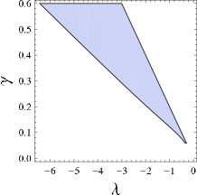
Figure 1: The allowed regions (shaded areas) for the parameters $\gamma$ and $\lambda$ for (a) $D=5$, (b) $D=6$, and (c) $D=10$. The upper boundary comes from that the asymptotically AdS boundary condition, and the lower boundary comes from the BF bound condition (41).

5 Hyperbolic topological black hole solutions with $k=-1$

We now present our numerical solutions for $k=-1$ with a positive cosmological term. We integrate the field equations from the event horizon to AdS infinity. The first step in the procedure is to choose appropriate radius of the event horizon $\tilde{r}_{H}$. Next we choose the value of $\phi_{H}$ and determine the values of other fields by Eqs. (15) and (17). Since the asymptotic behavior (35) is in general not satisfied for most of the values $\phi_{H}$, it should be tuned such that $\phi_{-}=0$ is achieved. We also fix $\delta_{H}=0$ in the integration and this would give nonzero $\delta_{0}$. However, $\delta_{0}=0$ is always realized by the shift symmetry (12). As a result, there is only one freedom of choosing $\tilde{r}_{H}$, given a cosmological constant. The solutions are obtained for the particular choice of $\gamma$ and $\lambda$, but we expect that qualitative properties do not change for other choices of these parameters unless $\gamma$ is too large, [10] though there is an indication that the range of the horizon radii for the existence of the black hole solutions changes depending on the strength of the dilaton coupling $\gamma$ [20]. In this section we fix $\gamma=1/2$. Using the symmetry in Eq. (11), the solutions for different values of cosmological constant can be generated from a solution for $\tilde{\Lambda}=+1$. Indeed, solutions for $\tilde{\Lambda}_{1}$ can be obtained by simply changing the variables as

$$\tilde{r}\to|\tilde{\Lambda}_{1}|^{-\frac{\gamma}{2(\lambda-\gamma)}}\tilde{r},~{}~{}~{}~{}~{}\phi\to\phi-\frac{1}{\lambda-\gamma}\log|\tilde{\Lambda}_{1}|,~{}~{}~{}~{}~{}\tilde{m}_{g}\to|\tilde{\Lambda}_{1}|^{-\frac{(D-3)\gamma}{2(\lambda-\gamma)}}\tilde{m}_{g}.$$ (42)

In the following subsections, we present numerical solutions in various dimensions. Before doing that, let us consider the analytical solution. It can be confirmed that the basic equations have the exact solution

$$\phi\equiv\phi_{0},~{}~{}\delta\equiv 0,~{}~{}B=\tilde{b}_{2}\tilde{r}^{2}-1,$$ (43)

where the relation of the parameters $b_{2}$, $\phi_{0}$ and the cosmological constant are given as Eqs. (29) and (30). This solution has an event horizon at $\tilde{r}=1/\sqrt{\tilde{b}_{2}}$, which coincides with the AdS radius $\ell_{\rm AdS}$. By Eq. (37), the mass of the black hole solution is $\tilde{m}_{g}\equiv\tilde{M}_{0}=0$. Hence this solution is the zero mass black hole. The center of the solution is not singular but regular.

Let us examine the boundary condition (17) in more detail here. It is a quadratic equation with respect to $\phi_{H}^{\prime}$. To guarantee the reality of $\phi_{H}^{\prime}$, we find that there are forbidden parameter regions of ($\phi_{H}^{\prime}$, $\tilde{r}_{H}$). Such regions (or allowed regions) are depicted in Fig. 2 for our choice of parameters $\gamma$, $\lambda$ and $\tilde{\Lambda}$ in each dimension. The solutions can exist only in those shaded regions. This does not, however, mean that there are always solutions for those values in these regions. We also mention that the regions seem to change depending on the parameter choice of $\gamma$ and $\lambda$, [20] but we will not discuss this issue in this paper.

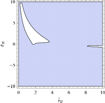
Figure 2: The region where Eq. (17) has real roots of $\phi_{H}^{\prime}$ (shaded area) for $\tilde{\Lambda}=1$, $\gamma=1/2$, and $k=-1$ in (a) $D=5$ ($\lambda=-3$), (b) $D=6$ ($\lambda=-2$), and (c) $D=10$ ($\lambda=-1$). On the boundary $\phi_{H}^{\prime}$ degenerates. Only in this region, regularity at the event horizon can be satisfied.

There is another boundary condition (14) which should be considered when we choose the value of $\phi_{H}$. The region where $B^{\prime}_{H}>0$ is shown in Fig. 3. Outside of the shaded region, the horizon, if it exists, is of cosmological horizon type.

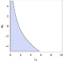
Figure 3: The region where $B^{\prime}_{H}>0$ for each solution of $\phi^{\prime}_{H}$ for $\tilde{\Lambda}=1$, $\gamma=1/2$, and $k=-1$ in (a), (a^′) $D=5$ ($\lambda=-3$), (b), (b^′) $D=6$ ($\lambda=-2$), and (c), (c^′) $D=10$ ($\lambda=-1$).

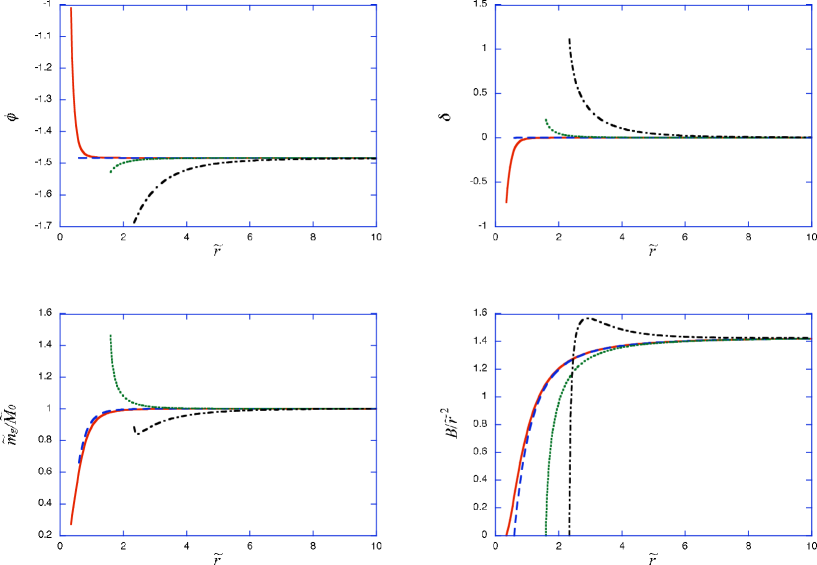
Figure 4: Behaviors of (a) the dilaton field $\phi(\tilde{r})$, (b) the lapse function $\delta(\tilde{r})$, (c) the mass function $\tilde{m}_{g}(\tilde{r})/\tilde{M}_{0}$, and (d) the metric function $B$ of the black hole solutions with $k=-1$ in $D=5$. The horizon radii and the masses are $\tilde{r}_{H}=0.35$, $\tilde{M}_{0}=-0.18614$ (solid line), $\tilde{r}_{H}=0.6$, $\tilde{M}_{0}=-0.13238$ (dashed line), $\tilde{r}_{H}=1.6$, $\tilde{M}_{0}=2.3287$ (dotted line), and $\tilde{r}_{H}=2.35$, $\tilde{M}_{0}=21.523$ (dot-dashed line).

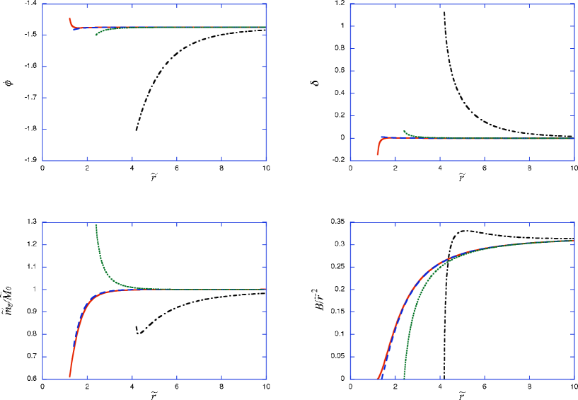
Figure 5: Behaviors of (a) the dilaton field $\phi(\tilde{r})$, (b) the lapse function $\delta(\tilde{r})$, (c) the mass function $\tilde{m}_{g}(\tilde{r})/\tilde{M}_{0}$, and (d) the metric function $B$ of the black hole solutions with $k=-1$ in $D=6$. The horizon radii and the masses are $\tilde{r}_{H}=1.22$, $\tilde{M}_{0}=-0.78098$ (solid line), $\tilde{r}_{H}=1.4$, $\tilde{M}_{0}=-0.68890$ (dashed line), $\tilde{r}_{H}=2.4$, $\tilde{M}_{0}=4.4924$ (dotted line), and $\tilde{r}_{H}=4.2$, $\tilde{M}_{0}=205.39$ (dot-dashed line).

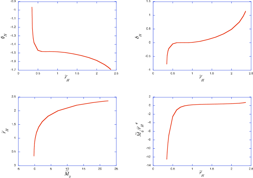
Figure 6: Numerical values of the fields (a) $\phi_{H}$ and (b) $\delta_{H}$ at the horizon and (c) the mass of the black hole $\tilde{M}_{0}$-$\tilde{r}_{H}$ diagram for $D=5$ and $k=-1$. (d) shows the scaled mass by horizon radius.

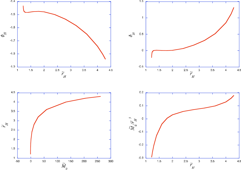
Figure 7: Numerical values of the fields (a) $\phi_{H}$ and (b) $\delta_{H}$ at the horizon and (c) the mass of the black hole $\tilde{M}_{0}$-$\tilde{r}_{H}$ diagram for $D=6$ and $k=-1$. (d) shows the scaled mass by horizon radius.

5.1 $D=5$ and $D=6$ solutions

First we present the black hole solutions in $D=5$ and $D=6$ simultaneously since the qualitative features of these solutions are similar. As the typical choice of parameters, we fix $\lambda=-3$ for $D=5$ and $\lambda=-2$ for $D=6$. These values are chosen in the allowed region given in Fig. 1. We find from Eqs. (29) and (30) that the square of inverse AdS radius and the asymptotic value of the dilaton field are $\tilde{b}_{2}=1.42869$ ($\ell_{\rm AdS}=0.8366$) and $\phi_{0}=-1.4837$ for $D=5$, and $\tilde{b}_{2}=0.318784$ ($\ell_{\rm AdS}=1.7711$) and $\phi_{0}=-1.47555$ for $D=6$, respectively.

The configurations of the field functions of the black hole solutions are depicted in Fig. 4 ($D=5$) and Fig. 5 ($D=6$). For the black holes with larger mass than that of the exact solution whose horizon radius is $\tilde{r}_{H}=\ell_{\rm AdS}$, the dilaton field increases monotonically to its asymptotic value $\phi_{0}$. Although the mass function decreases near the event horizon, it increases asymptotically. The function $\delta$ monotonically decreases. As the radius of solution becomes large, we see that $B$ becomes steep around the black hole horizon. For the small black holes $\tilde{r}_{H}=0.6$ ($D=5$) and $\tilde{r}_{H}=1.22$ ($D=6$), the dilaton field decreases for the domain where $\tilde{r}\lesssim\ell_{\rm AdS}$. The mass function decreases in most of the spacetime region although it increases asymptotically (Note that $m_{g}(r)/M_{0}$ increases while $m_{g}(r)$ itself decreases when $M_{0}$ is negative). The function $\delta$ monotonically increases. Hence the qualitative features of the solutions change for $\tilde{r}_{H}\approx\ell_{\rm AdS}$.

The plots of $\phi_{H}$, $\delta_{H}$, and $\tilde{M}_{0}$ as functions of $\tilde{r}_{H}$ are given in Fig. 6 ($D=5$) and Fig. 7 ($D=6$). It is noted that the black hole solution exists only for $0.3496<\tilde{r}_{H}<2.36$ ($D=5$) and $1.218<\tilde{r}_{H}<4.3$ ($D=6$).

In the non-dilatonic case, there are also bounds for the existence of the black hole solutions. In $D=5$, the lower bound is zero horizon radius where a naked singularity appears, and the upper bound is determined by the appearance of the branch singularity at finite radius[21]. In $D=6$, the lower bound is the extreme black hole solution where the horizons degenerate, and the upper bound is the branch singularity as in $D=5$. In the dilatonic case, for the solution at the lower bound, the second derivative of the dilaton field $\phi^{\prime\prime}$ diverges at the horizon while $B^{\prime}_{H}$ and $\delta_{H}$ are finite. For the solution at the upper bound, $h_{H}$ becomes zero and $B^{\prime}_{H}$ diverges. The Hawking temperature is given by the periodicity of the Euclidean time on the horizon as

$$\tilde{T}_{H}~{} =\frac{e^{-\delta_{H}}}{4\pi}B_{H}^{\prime}$$ (44)

$$=\frac{e^{-\delta_{H}}}{4\pi h_{H}}\biggl{[}\frac{(D-3)k}{\tilde{r}_{H}}+\frac{(D-3)_{5}k^{2}}{\tilde{r}_{H}^{2}}e^{-\gamma\phi_{H}}-\frac{\tilde{r}_{H}\tilde{\Lambda}e^{\lambda\phi_{H}}}{D-2}\biggr{]}.$$

Hence the temperature of the black hole in the upper bound becomes infinite. If we try to add the mass to the black hole to get the larger black hole than upper bound, the emission rate of the black hole is extremely large and the black hole may remain smaller than the upper bound. The qualitative behavior of the physical quantities in Figs. 6 and 7 seems to be divided by zero mass exact solution (43). The gravitational mass $\tilde{M}_{0}$ is monotonic with respect $\tilde{r}_{H}$. For the large black holes $\tilde{M}_{0}\sim\tilde{r}_{H}^{D-1}$ as in the non-dilatonic case, while it grows faster for the small black holes.

5.2 $D=10$ solution

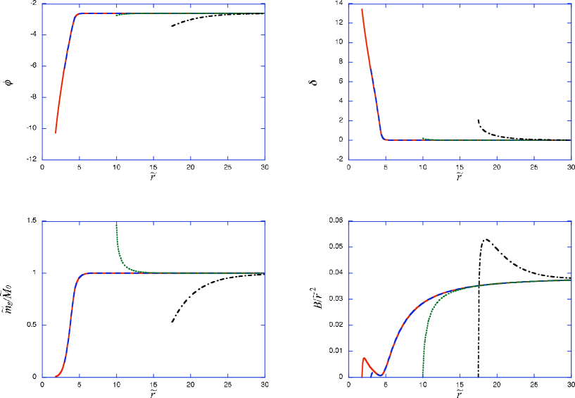
Figure 8: Behaviors of (a) the dilaton field $\phi(\tilde{r})$, (b) the lapse function $\delta(\tilde{r})$, (c) the mass function $\tilde{m}_{g}(\tilde{r})/\tilde{M}_{0}$, and (d) the metric function $B$ of the black hole solutions with $k=-1$ in $D=10$. The horizon radii and the masses are $\tilde{r}_{H}=1.8$, $\tilde{M}_{0}=-4919.2$ (solid line), $\tilde{r}_{H}=3.0$, $\tilde{M}_{0}=-4909.1$ (dashed line), $\tilde{r}_{H}=10.0$, $\tilde{M}_{0}=9.7349\times 10^{6}$ (dotted line), and $\tilde{r}_{H}=17.5$, $\tilde{M}_{0}=5.1025\times 10^{9}$ (dot-dashed line).

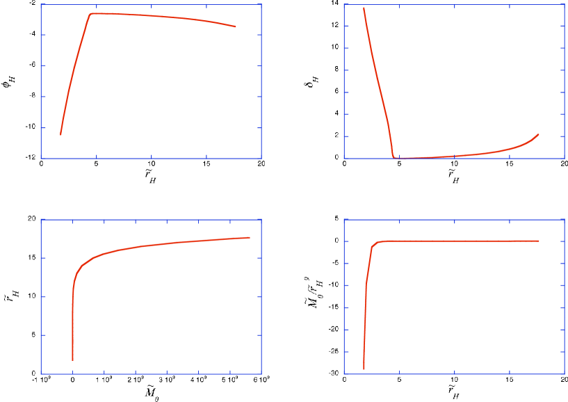
Figure 9: Numerical values of the fields (a) $\phi_{H}$ and (b) $\delta_{H}$ at the horizon and the mass of the black hole (c) $\tilde{M}_{0}$-$\tilde{r}_{H}$ diagram in $D=10$. (d) shows the scaled mass by horizon radius. For each figure, $k=-1$.

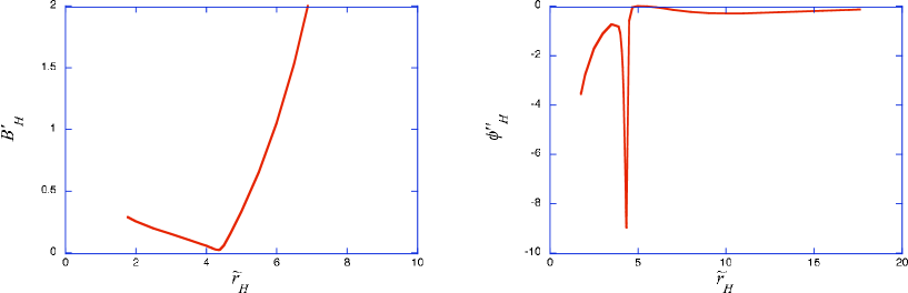
Figure 10: Numerical values of the fields (a) $B^{\prime}_{H}$ and (b) $\phi^{\prime\prime}_{H}$ in $D=10$. For each figure, $k=-1$.

The properties of the black hole solutions in 10-dimensional spacetime are different from those in $D=5$ and $6$ cases. We choose $\lambda=-1$. From Eqs. (29) and (30), we find that the square of inverse AdS radius and the asymptotic value of the dilaton field are $\tilde{b}_{2}=0.038415$ ($\ell_{\rm AdS}=5.1021$) and $\phi_{0}=-2.6268$, respectively.

The configurations of the field functions of the black hole solutions are given in Fig. 8. For the solutions with $\tilde{r}_{H}=10.0$ and $17.5$, the dilaton field increases monotonically to its asymptotic value $\phi_{0}=0$. The mass function for $\tilde{r}_{H}=17.5$ monotonically increases while it decreases near the event horizon and increases asymptotically for smaller black holes. As the solution becomes large, we find that $B$ becomes steep around the event horizon. The functions $\phi$, $\delta$, and $m_{g}$ have almost the same configurations for the solutions with $\tilde{r}_{H}=1.8$ and $3.0$, i.e., the functions for $\tilde{r}_{H}=1.8$ and $3.0$ trace the same curves on the figures. The metric function $B$ approaches zero at the local minimum around $\tilde{r}=\tilde{r}^{\ast}\approx 4.36$ ($B^{\prime}$ becomes zero there) and bounces to $B/\tilde{r}^{2}\to\tilde{b}_{2}$. So the solution looks like extreme black hole from outside. This is the common property for the solutions with horizon radius smaller than $\tilde{r}^{\ast}$.

We show $\phi_{H}$, $\delta_{H}$, and $\tilde{M}_{0}$ as functions of $\tilde{r}_{H}$ in Fig. 9. The black hole solution exists only for limited range of horizon radius $1.76<\tilde{r}_{H}<17.61$. The $\phi_{H}$-$\tilde{r}_{H}$ plot and $\delta_{H}$-$\tilde{r}_{H}$ plot have cusp like structures at the horizon radius $\tilde{r}_{H}=\tilde{r}^{\ast}$. This radius is smaller than the AdS radius $\ell_{\rm AdS}=5.1021$. When the horizon radius is larger than $\tilde{r}^{\ast}$, the solutions have similar properties to those of the large black holes in $D=5$ and $6$. $\phi_{H}$ monotonically decreases and $\tilde{M}_{0}\sim\tilde{r}_{H}^{D-1}$ asymptotically. For the largest $\tilde{r}_{H}=17.61$, $B^{\prime}_{H}$ diverges, which means that the temperature of the black hole also diverges. For solutions with $\tilde{r}_{H}$ smaller than $\tilde{r}^{\ast}$, the solutions have different properties from large one. $\phi_{H}$ and $\delta_{H}$ seem to be linear to $\tilde{r}_{H}$. The solution disappears at the lower bound $\tilde{r}_{H}=1.76$, where the non-normalizable mode of the dilaton field cannot be eliminated by tuning the shooting parameter $\phi_{H}$.

For the horizon radius $\tilde{r}_{H}=\tilde{r}^{\ast}$, the value $B^{\prime}_{H}$ vanishes (See Fig. 10 (a)), which means that the horizon degenerates. However, this is not an extreme black hole solution with a regular horizon because the second derivative of the dilaton field diverges (See Fig. 10 (b)).

6 Planar topological black hole solution with $k=0$

The basic equations have the following exact solution

$$\phi\equiv\phi_{0},~{}~{}\delta\equiv 0,~{}~{}B=\tilde{b}_{2}\tilde{r}^{2},$$ (45)

where the relation of the parameters $b_{2}$ and $\phi_{0}$ are again given as Eqs. (29) and (30). For $\gamma>(D-4)|\lambda|/D$, $\tilde{b}_{2}$ is negative and the metric function $B$ is negative semidefinite. So this solution is physically less interesting. For $\gamma<(D-4)|\lambda|/D$, $\tilde{b}_{2}$ is positive. The spacetime is regular everywhere and approaches the AdS spacetime asymptotically.

It can be proved simply that there is no black hole solution with $k=0$. In the $k=0$ case, Eq. (15) becomes

$$B_{H}^{\prime}=-\frac{\tilde{r}_{H}\tilde{\Lambda}e^{\lambda\phi_{H}}}{D-2}<0.$$ (46)

This means that the horizon is not the black hole horizon but the cosmological horizon type which is not the solution we are looking for. Hence there is no black hole solution in this case.

7 Spherically symmetric black hole solutions with $k=1$

It can be confirmed that the basic equations have the exact solution

$$\phi\equiv\phi_{0},~{}~{}\delta\equiv 0,~{}~{}B=\tilde{b}_{2}\tilde{r}^{2}+1,$$ (47)

where the relation of the parameters $b_{2}$ and $\phi_{0}$ are again given as Eqs. (29) and (30). For $\gamma>(D-4)|\lambda|/D$, the solution is regular dS solution. In the $k=-1$ case, there is also an exact solution (43) which is a zero-mass black hole solution. By adding static perturbations around that solution, the black hole solutions with the nontrivial dilaton field and infinitesimal mass are obtained. Similarly, it might be expected that the regular solution with a nontrivial dilaton field is obtained by static perturbations in the $k=1$ case. It could be a new nontrivial solution with a cosmological horizon. At the cosmological horizon, the dilaton field should satisfy the regularity condition, and the degree of freedom of the dilaton field at the center is used to realize this. Unfortunately then, the growing mode in the dilaton field that arises asymptotically as discussed in § 4.2 cannot be eliminated since the freedom is already used up. There is certianly a possibility that this might happen to vanish, but this is not expected in general. Hence such an asymptocic dS black hole solution, if it could exist for very particular set of parameters, may have little importance physically.

For $\gamma<(D-4)|\lambda|/D$, the solution is AdS solution. Depending on the parameters, the solution satisfies the BF bound. By adding static perturbations to this exact solution, we may obtain an everywhere regular solution with non-trivial dilaton field in the asymptotically AdS spacetime. In this case, there is no cosmological horizon and we have the freedom to kill the growing mode and obtain the good asymptotic AdS behavior. Though this is not a black hole solution, it is an interesting solution in its own right. We will report on this possibility in the near future.

As in the topological black hole case ($k=-1$), we made various choices of the parameters of the theory $\gamma$ and $\lambda$, and integrated the field equations from $\tilde{r}=\tilde{r}_{H}$ to see if there is an asymptotically AdS black hole solution. The metric function $B$ grows from zero and takes local maximum and then decreases. As $B$ approaches zero, the field equations become singular, and $\phi$ and $B$ seem to diverge at finite radius. Thus, even if we succeed in getting $B=0$ corresponding to the cosmological horizon by tuning $\phi_{H}$, the spacetime does not approach AdS spacetime. This means that the spacetime is singular, and suggests that there is no such solution. Having searched for improved solutions by changing the parameters of theory $\gamma$, $\lambda$, the physical parameter $r_{H}$ and shooting parameter $\phi_{H}$, we have not found any reasonable solution after long struggle. Together with the above discussions on the general behaviors of the function $B$, we conclude that it is very unlikely that there is any asymptotically AdS black hole solution in $k=1$ case with positive cosmological constant.

8 Hyperbolic topological solutions with $k=-1$ without cosmological constant

In this series of our papers, there still remains a case that has not been investigated. It is the case of $k=-1$ and zero cosmological constant. Here we briefly report on our study of this case.

The basic equations are obtained by putting $k=-1$ and $\tilde{\Lambda}=0$ in Eqs. (3)-(9). These equations have the same symmetry properties and scaling rules as Eqs (10)-(12). In particular, the shift symmetry (11) is written as

$$\phi\to\phi-\phi_{\ast},~{}~{}r\to e^{-\gamma\phi_{\ast}/2}r,~{}~{}\delta\to\delta,~{}~{}B\to B.$$ (48)

This can be used to shift the asymptotic value of the dilaton field to zero even when we compute the metric functions and the dilaton field for any boundary value $\phi_{H}$ at the horizon. In other words, we can first fix the horizon radius, for example, $\tilde{r}_{H}=1$, and obtain various solutions with different $\phi_{H}$. Then applying the shift symmetry (48), we can obtain the solutions with various horizon radii and zero dilaton field at infinity.

In the non-dilatonic case, there are two branches of the solutions with $\Lambda=0$ and $k=-1$[21]. The GR branch does not give a black hole solution while there are black hole solutions for some mass range in the GB branch. Such black hole solutions have asymptotic AdS structure. If there is a black hole solution in the dilatonic system, it cannot have AdS structure for the following reason. In the AdS spacetime, the GB term becomes dominant asymptotically and it can be regarded as the Liouville type potential of the dilaton field. Hence the potential does not have extremum, and the dilaton field diverges. This means that a black hole solution, if it exists, does not approach the non-dilatonic solutions in the non-dilatonic limit ($\gamma\to 0$) and it should be new type of solutions.

We assume the same boundary conditions 1-3 in § 3. At the horizon, Eq. (15) becomes

$$B_{H}^{\prime}=-\frac{1}{h_{H}}\biggl{[}\frac{(D-3)}{\tilde{r}_{H}}+\frac{(D-4)_{5}C}{2}\biggr{]}.$$ (49)

This must be positive for the existence of the black hole horizon. In $D=4$, Eq. (49) becomes

$$B_{H}^{\prime}=-\frac{1}{h_{H}\tilde{r}_{H}}.$$ (50)

For $D=4$, Eq. (17) gives

$$h_{H}^{2}-h_{H}+6\gamma^{2}C^{2}=0,$$ (51)

whose two solutions are, if they are real, both positive. Hence $B^{\prime}_{H}$ is always negative, excluding the existence of the black hole solution in $D=4$. In $D\geq 5$, Eq. (17) is too complicated to deduce definite conclusion. So we fix the value of $\gamma$ and examine the positivity of $B^{\prime}_{H}$. Figs. 11 are the plots of $B^{\prime}_{H}$ as a function of $\phi_{H}$ for $\gamma=1/2$. $\tilde{r}_{H}$ is fixed to $\tilde{r}_{H}=1$ by the scaling property of the system. We find there is a narrow range where $B^{\prime}_{H}$ becomes positive. However, integrating the field equations from $\tilde{r}=1$ with $\phi_{H}$ in this range, we find that calculation stops, and the field variables diverge. This gives a rather strong evidence that there is no black hole solution in this case either.

Figure 11: The $B^{\prime}_{H}$-$\phi_{H}$ plots for each solution for $\Lambda=0$, $\gamma=1/2$, $k=-1$, and $\tilde{r}_{H}=1$ in $D=5$ ((a) and (a^′)) and $D=10$ ((b) and (b^′)). Two plots in each dimension correspond to two roots for $\phi^{\prime}_{H}$ in Eq. (17). The range for $\phi^{\prime}_{H}$ with no plot implies that $\phi^{\prime}_{H}$ becomes imaginary.

9 Discussions and Conclusions

We have studied the black hole solutions in the dilatonic Einstein-GB theory with the positive cosmological constant. The cosmological constant introduces the Liouville type of potential for the dilaton field with a certain coupling. We have studied the spherically symmetric ($k=1$), planar symmetric ($k=0$), and hyperbolically symmetric ($k=-1$) spacetimes in various dimensions.

The black hole solution should have a regular black hole horizon and be singularity free in the outer region. Due to the presence of the positive cosmological constant, it is expected that the cosmological horizon appears. To obtain the regular cosmological horizon, the boundary value of the dilaton field at the black hole horizon should be tuned. However, it is found by the asymptotic expansion at infinity that the dilaton field has a non-normalizable mode for such solutions. As a result, there is no physically relevant black hole solutions in asymptotically dS spacetime generically.

In the planar symmetric spacetime, all the horizons become the cosmological horizon type, i.e., $B^{\prime}_{H}<0$, which means that there is no black hole solution.

In the spherically symmetric and the hyperbolically symmetric spacetimes, there are parameter regions where the solutions can have asymptotically AdS spacetimes. By the asymptotic expansion at infinity, the power decaying rate of the fields are estimated. We have imposed the condition that the “mass” of the dilaton field satisfies the BF bound, which guarantees the stability of the vacuum solution. By this condition, the values of the dilaton coupling constant and the parameter of the Liouville potential are constrained.

In the spherically symmetric spacetime, however, we could not find any solution with AdS asymptotics numerically, and concluded that there is no black hole solution with $k=1$ in this system.

On the other hand, we were able to construct AdS black hole solutions in hyperbolically symmetric spacetime in higher dimensions ($D\geq 5$) numerically. The basic equations have some symmetries which are used to generate the black hole solutions with different horizon radii and the cosmological constants. We have chosen $\gamma=1/2$ and $\lambda=-3$ ($D=5$), $\lambda=-2$ ($D=6$), and $\lambda=-1$ ($D=10$), for the actual numerical analysis. The field equations have exact solutions, i.e., a massless black hole solution with the constant dilaton field.

The black hole solutions in the $D=5$ and $D=6$ spacetimes have similar properties. Configurations of the field functions change qualitatively depending on whether the size of the black hole is larger than the AdS radius or not. For the small black holes, the GB term becomes efficient, and the solutions deviate from the non-dilatonic one. The black hole solutions exist for a certain range of the size of horizon radius. At the lower bound, the second derivative of the dilaton field diverges at the horizon, and there appears a singularity at finite radius. This is similar to the spherically symmetric black hole solution without the cosmological constant. [1, 9] At the upper bound, the derivative of the metric function $B^{\prime}$ diverges at the horizon. The temperature of the black hole becomes infinite.

In the $D=10$ spacetimes there is a special solution, which is singular, for the horizon radius $\tilde{r}^{\ast}$. Since the derivative of the metric function $B^{\prime}$ vanishes at the black hole horizon, the solution looks similar to the extreme black hole solution. However, it is not extreme one because the second derivative of the dilaton field diverges. When the horizon radius is larger than $\tilde{r}^{\ast}$, the solutions have similar properties to the large solutions in lower dimensions $D=5$ and $6$. There is an upper bound for the horizon radius where $B^{\prime}_{H}$ diverges. When the horizon radius is smaller than $\tilde{r}^{\ast}$, it is interesting that the configurations of the field functions trace the similar curves to those of the solution with the horizon radius $\tilde{r}_{H}=\tilde{r}^{\ast}$ outside of $\tilde{r}^{\ast}$. The solutions disappear at the lower bound, where the non-normalizable mode of the dilaton field cannot be eliminated by tuning the value of $\phi_{H}$.

The characteristic feature of the solutions in this model is the existence of the upper bound for the size of the black holes. If the matter which has more mass than the upper bound, i.e., macroscopic size compared to the string scale, collapses gravitationally, the final state is not the static black hole but something else. One of the candidates is the appearance of the naked singularity, which is an undesirable situation physically. Another possibility is that the matter field does not collapse to form the black hole and the spacetime remains regular everywhere like a soliton or a lump solution. This is allowed since the GB term breaks the energy condition if it is regarded as the “matter part” in GR and the singularity theorem does not apply. This is a kind of singularity avoidance.

We have also studied the hyperbolically symmetric black hole solutions without the cosmological constant which was not investigated in our previous papers. In the $D=4$ case, it is proved that all the horizon is of the cosmological horizon type and that there is no black hole solution. In the higher dimensional cases, it appears that the solution can have a black hole horizon. However, the parameter region for the suitable boundary conditions is very narrow, and we did not find any black hole solution in this case.

Since this is the final paper of our series about the dilatonic black hole solutions in various dimensions, it is helpful to summarize the results obtained in our papers. We show some properties of the solutions in Table 1 in $D=4,\>5,\>6,$ and 10 spacetimes. In the $\Lambda=0$ case, there is a black hole solutions only for spherically symmetric ($k=1$) spacetime. The solutions are asymptotically flat and there is the lower bound for the size of the horizon in $D=4,5$, and $6$ but there is not such a bound in $D=10$.

Table 1: Summary of the black hole solutions in the dilatonic Einstein-Gauss-Bonnet theory in various dimensions. The head “existence” shows the existence of the black hole solution which satisfy appropriate boundary conditions. For the $\Lambda=0$, $k=-1$ and the $\Lambda=1$, $k=1$ cases, “no” means that the non-existence of the solution cannot be proved exactly but we cannot find the solution numerically. For the $\Lambda=1$, $k=-1$ case, there are solutions for $D=5,6$, and 10 but there is no solution for $D=4$. The head “asymptotics” shows the asymptotic structure of the solution. There is no asymptotically dS solution generically. The head “lower bound” and “upper bound” show the existence of the lower and upper bounds for the horizon radius. For the $\Lambda=1$, $k=1$ case, there is the lower bound for $D=4,\>5$ but no bound for $D=6,\>10$. The head “paper” shows the number in the series of our paper where the model is discussed.

	$k$	existence	asymptotics	lower bound	upper bound	paper
				yes ($D=4,\>5$)
	$k=1$	yes	flat	no ($D=6,\>10$)	no	I
$\Lambda=0$	$k=0$	no	—–	—–	—–	II
	$k=-1$	“no”	—–	—–	—–	IV
	$k=1$	“no”	—–	—–	—–	IV
	$k=0$	no	—–	—–	—–	IV
$\Lambda=1$		yes ($D\geq 5$)
	$k=-1$	no ($D=4$)	AdS	yes	yes	IV
	$k=1$	yes	AdS	yes	no	III
$\Lambda=-1$	$k=0$	yes	AdS	no	no	II
	$k=-1$	yes	AdS	yes	no	III

For the positive cosmological term, the black hole solutions exist only for hyperbolically symmetric ($k=-1$) and $D=5,\>6,\>10$ spacetimes and there is no black hole solution in $D=4$. We have obtained the allowed parameter region of $\gamma$ and $\lambda$ for the existence of the solutions. In spite of the positive cosmological constant, the spacetime is asymptotically AdS. There are both the upper and lower bounds on the size of the black hole.

For the negative cosmological term, there are black hole solutions for all $k$. We have found the allowed parameter region of $\gamma$ and $\lambda$ for the existence of the solutions. They are asymptotically AdS and do not have upper bound for the size of the event horizon. There is no lower bound on the horizon for the $k=0$ solutions while there is for the $k=\pm 1$ solutions as in the $\Lambda=0$ and $k=1$ case.

Non-existence of the black hole solution in asymptotically dS spacetime is strongly related to the cosmological horizon. The equation of the dilaton field becomes singular at horizons, and regularity of the horizons gives constraints on the dilaton field and its derivative. To satisfy these constraints, the dilaton field has to have suitable value at each horizons. There is another boundary condition, i.e., the asymptotic behavior at infinity. This gives a further constraint on the dilaton field. However, there is no freedom to satisfy all the constraints at more than one horizon and at infinity simultaneously. This is the basic reason why there is no asymptotically dS black hole solution in this system. In general, it is expected that the system of the matter field whose equation of motion is singular at the horizons cannot have a black hole solution in asymptotically dS spacetime for a similar reason.

For the non-dilatonic black holes in the Einstein-Gauss-Bonnet theory, global structures of all the static solutions with $k=\pm 1$ and $k=0$ are investigated[21]. Since our numerical analysis was limited to outer spacetime of the event horizon, the global structures of the solutions such as the existence of the inner horizon, and the singularity have not been clarified. This is left for future study.

The stability of our solutions is another important subject. [22] For the $\Lambda=0$ and $k=1$ case in $D=4$, the stability against the spherically symmetric perturbations is examined[23]. In the non-dilatonic case, it was found that the black hole solutions are stable against the spherical perturbations but can be unstable against the non-spherical perturbations for the small solutions[24, 25]. It is interesting to see whether the effects of the dilaton field can stabilize the solutions.

References

- [1] Z. K. Guo, N. Ohta and T. Torii, “Black Holes in the Dilatonic Einstein-Gauss-Bonnet Theory in Various Dimensions I – Asymptotically Flat Black Holes –,” Prog. Theor. Phys. 120 (2008) 581 [arXiv:0806.2481 [gr-qc]].
- [2] Z. K. Guo, N. Ohta and T. Torii, “Black Holes in the Dilatonic Einstein-Gauss-Bonnet Theory in Various Dimensions II – Asymptotically AdS Topological Black Holes –,” Prog. Theor. Phys. 121 (2009) 253 [arXiv:0811.3068 [gr-qc]].
- [3] N. Ohta and T. Torii, “Black Holes in the Dilatonic Einstein-Gauss-Bonnet Theory in Various Dimensions III – Asymptotically AdS Black Holes with –,” Prog. Theor. Phys. 121 (2009) 959 [arXiv:0902.4072 [hep-th]].
- [4] G. W. Gibbons and K. Maeda, “Black Holes And Membranes In Higher Dimensional Theories With Dilaton Fields,” Nucl. Phys. B 298 (1988) 741.
- [5] D. Garfinkle, G. T. Horowitz and A. Strominger, “Charged black holes in string theory,” Phys. Rev. D 43 (1991) 3140.
-
[6]
R. R. Metsaev and A. A. Tseytlin,
“Order alpha-prime (Two Loop) Equivalence of the String Equations of Motion
and the Sigma Model Weyl Invariance Conditions: Dependence on the Dilaton and
the Antisymmetric Tensor,”
Nucl. Phys. B 293 (1987) 385;
D. J. Gross and J. H. Sloan, “The Quartic Effective Action for the Heterotic String,” Nucl. Phys. B 291 (1987) 41. - [7] P. Kanti, N. E. Mavromatos, J. Rizos, K. Tamvakis and E. Winstanley, “Dilatonic Black Holes in Higher Curvature String Gravity,” Phys. Rev. D 54 (1996) 5049 [arXiv:hep-th/9511071].
- [8] S. O. Alexeev and M. V. Pomazanov, “Black hole solutions with dilatonic hair in higher curvature gravity,” Phys. Rev. D 55 (1997) 2110 [arXiv:hep-th/9605106].
- [9] T. Torii, H. Yajima and K. Maeda, “Dilatonic black holes with Gauss-Bonnet term,” Phys. Rev. D 55 (1997) 739 [arXiv:gr-qc/9606034].
- [10] C. M. Chen, D. V. Gal’tsov and D. G. Orlov, “Extremal black holes in D = 4 Gauss-Bonnet gravity,” Phys. Rev. D 75 (2007) 084030 [arXiv:hep-th/0701004].
- [11] C. M. Chen, D. V. Gal’tsov and D. G. Orlov, “Extremal dyonic black holes in D=4 Gauss-Bonnet gravity,” arXiv:0809.1720 [hep-th].
- [12] D. G. Boulware and S. Deser, “String Generated Gravity Models,” Phys. Rev. Lett. 55 (1985) 2656.
-
[13]
J. T. Wheeler,
“Symmetric Solutions To The Gauss-Bonnet Extended Einstein Equations,”
Nucl. Phys. B 268 (1986) 737;
D. L. Wiltshire, “Spherically Symmetric Solutions Of Einstein-Maxwell Theory With A Gauss-Bonnet Term,” Phys. Lett. B 169 (1986) 36;
R. C. Myers and J. Z. Simon, “Black Hole Thermodynamics in Lovelock Gravity,” Phys. Rev. D 38 (1988) 2434;
G. Giribet, J. Oliva and R. Troncoso, “Simple compactifications and black p-branes in Gauss-Bonnet and Lovelock theories,” JHEP 0605 (2006) 007 [arXiv:hep-th/0603177];
R. G. Cai and N. Ohta, “Black holes in pure Lovelock gravities,” Phys. Rev. D 74 (2006) 064001 [arXiv:hep-th/0604088].
For reviews and references, see C. Garraffo and G. Giribet, “The Lovelock Black Holes,” arXiv:0805.3575 [gr-qc] and C. Charmousis, “Higher order gravity theories and their black hole solutions,” arXiv:0805.0568 [gr-qc]. - [14] R. G. Cai, “Gauss-Bonnet black holes in AdS spaces,” Phys. Rev. D 65 (2002) 084014 [arXiv:hep-th/0109133].
- [15] R. G. Cai, Z. Y. Nie, N. Ohta and Y. W. Sun, “Shear Viscosity from Gauss-Bonnet Gravity with a Dilaton Coupling,” arXiv:0901.1421 [hep-th].
- [16] L. Alvarez-Gaume, P. H. Ginsparg, G. W. Moore and C. Vafa, “An O(16) X O(16) Heterotic String,” Phys. Lett. B 171 (1986) 155.
- [17] J. Polchinski, “String theory,” Cambridge Univ. Pr. (1998).
- [18] K. Bamba, Z. K. Guo and N. Ohta, “Accelerating Cosmologies in the Einstein-Gauss-Bonnet Theory with Dilaton,” Prog. Theor. Phys. 118 (2007) 879 [arXiv:0707.4334 [hep-th]].
- [19] P. Breitenlohner and D. Z. Freedman, “Stability In Gauged Extended Supergravity,” Annals Phys. 144 (1982) 249.
- [20] K. Maeda, N. Ohta and Y. Sasagawa, “Black Hole Solutions in String Theory with Gauss-Bonnet Curvature Correction,” in preparation.
- [21] T. Torii and H. Maeda, “Spacetime structure of static solutions in Gauss-Bonnet gravity: Neutral case,” Phys. Rev. D 71 (2005) 124002 [arXiv:hep-th/0504127].
- [22] P. Pani and V. Cardoso, “Are black holes in alternative theories serious astrophysical candidates? The case for Einstein-Dilaton-Gauss-Bonnet black holes,” arXiv:0902.1569 [gr-qc].
- [23] T. Torii and K. i. Maeda, “Stability of a dilatonic black hole with a Gauss-Bonnet term,” Phys. Rev. D 58 (1998) 084004.
-
[24]
G. Dotti and R. J. Gleiser,
“Gravitational instability of Einstein-Gauss-Bonnet black holes under
tensor mode perturbations,”
Class. Quant. Grav. 22 (2005) L1
[arXiv:gr-qc/0409005];
G. Dotti and R. J. Gleiser, “Linear stability of Einstein-gauss-bonnet static spacetimes. part. I: Tensor perturbations,” Phys. Rev. D 72 (2005) 044018 [arXiv:gr-qc/0503117]. - [25] T. Takahashi and J. Soda, “Stability of Lovelock Black Holes under Tensor Perturbations,” Phys. Rev. D 79 (2009) 104025 [arXiv:0902.2921 [gr-qc]].