Typicality in random matrix product states

Abstract

Recent results suggest that the use of ensembles in Statistical Mechanics may not be necessary for isolated systems, since typically the states of the Hilbert space would have properties similar to the ones of the ensemble. Nevertheless, it is often argued that most of the states of the Hilbert space are non-physical and not good descriptions of realistic systems. Therefore, to better understand the actual power of typicality it is important to ask if it is also a property of a set of physically relevant states. Here we address this issue, studying if and how typicality emerges in the set of matrix product states. We show analytically that typicality occurs for the expectation value of subsystems’ observables when the rank of the matrix product state scales polynomially with the size of the system with a power greater than two. We illustrate this result numerically and present some indications that typicality may appear already for a linear scaling of the rank of the matrix product state.

I introduction

Statistical mechanics has been very successful in making predictions about the behavior of macroscopic systems we encounter in nature, yet there are still open questions concerning a fully quantum formulation of statistical mechanics. For instance, how can we explain the use of statistical ensembles in the description of a physical system which is supposed to be in a definite state? In this context the independent re-discovery by several groups of the importance of typicality GeMiMa ; Leb ; GoLeTu ; PoShWi has given rise to interesting directions of research Rei1 ; Rei2 ; RiDuOl ; Whi . Although the concept originally appeared as an incomplete formulation in a work by Schrodinger Sch , Lebowitz was the one to coin the term ’typicality’ and, together with others, did some pioneering work on the subject Leb ; GoLeTu . Typicality can be seen as a key feature justifying the effectiveness of standard equilibrium statistical mechanics, without requiring ergodicity or mixing. The works on typicality in the quantum setting have shown that ensemble averages and subjective ignorance may not be necessary concepts for the understanding of statistical mechanics PoShWi .

Intuitively, typicality refers to the fact that the vast majority of pure microstates of a quantum system, belonging to a well-defined region of the allowed state space, yield measurement outcomes very close to each other. More quantitatively, typicality can be associated with a very small variance of the measurement outcomes with respect to a specified ensemble of states.

Previous works PoShWi ; Rei1 ; Rei2 have focused on the study of typicality for general quantum states, providing a first alternative approach to the foundational problems of quantum statistical mechanics. However it is well know that the generation of Haar distributed random states is hard even at the quantum level EmWeSa . Therefore in order to consider typicality an effective scheme for the justification of statistical mechanics one should restrict to realizable random states, possibly with some specific physical content. First we need to choose and characterize this set of states, though of course the choice is not unique. In the present work we focus on Matrix Product States (MPS) (see Verstraete08 for a review and original references) as instances of physically accessible states. The reason why we restrict the study of typicality to MPS is because these are a good example of physically relevant states, arising as ground states of local Hamiltonians and being at the basis of some of the most recent and promising classical algorithms for the simulation of quantum systems Verstraete08 . Both of these properties justify a better understanding of their statistical properties with respect to typicality, which eventually can also lead to new powerful simulation techniques (as the work in Whi may suggest). We shall prove that typicality can emerge in the MPS set, and then illustrate this result with some numerical simulations.

II random matrix product states

A matrix product state is a pure one-dimensional quantum state whose coefficients are specified by a product of matrices. In the case of Periodic Boundary Conditions (PBC) an MPS can be written as

$$|\psi\rangle=\sum_{i_{1},...,i_{N}}{\rm Tr}\left[A^{i_{1}}[1]\cdots A^{i_{N}}[N]\right]|i_{1}\cdots i_{N}\rangle,$$

whereas for Open Boundary Conditions (OBC) we have

$$|\psi\rangle=\sum_{i_{1},...,i_{N}}\langle\phi_{I}|A^{i_{1}}[1]\cdots A^{i_{N}}[N]|\phi_{F}\rangle|i_{1}\cdots i_{N}\rangle,$$

with $|\phi_{I}\rangle$ and $|\phi_{F}\rangle$ specifying the states at the boundaries and $|i_{k}\rangle$ a local basis at site $k$. The matrices $\{A^{1}[s],A^{2}[s],\dots,A^{D}[s]\}$, with $s\in\{1,\dots,N\}$, are $\chi$-dimensional complex matrices, with $D$ the local Hilbert space dimension. For homogeneous MPS the set $\{A^{1}[s],A^{2}[s],\dots,A^{D}[s]\}$ is the same for all sites $s$. In the case of PBC they are referred to as Translationally Ivariant (TI) MPS. In the present work, for simplicity of notation and analysis, we deal numerically with OBC-MPS and analytically with PBC-TI-MPS. We checked numerically that all of our conclusions hold true independently of the boundary conditions and invariance under translations.

By definition, a MPS is specified by the set $\{A^{1},A^{2},\dots,A^{D}\}$, though there may exist a different set of matrices that form the same MPS. In PeVeWo it is shown that this sort of gauge degree of freedom can be fixed using a canonical form where the $A$ matrices satisfy two constraints: $\sum_{i=1}^{D}A^{i}A^{i\dagger}=\mathbb{I}$ and $\sum_{i=1}^{D}A^{i\dagger}\Lambda A^{i}=\Lambda$, for fixed $\Lambda$ (an alternative set of constraints is given by $\sum_{i=1}^{D}A^{i\dagger}A^{i}=\mathbb{I}$ and $\sum_{i=1}^{D}A^{i}\Lambda A^{i\dagger}=\Lambda$, see PeVeWo for details). MPS can also be seen as generalized valence-bond states Verstraete08 , and as such, emerging from the projection on some virtual or ancillary Hilbert space. The fundamental parameter of an MPS is the size $\chi$ of the $A$-matrices. In general, an MPS contains $ND\chi^{2}$ parameters, much less than the usual $D^{N}$ of a general state, and as a consequence the maximum entanglement a subsystem can have with its environment depends on $\chi$. It can be shown that any state can be described as an MPS for large enough $\chi$ with at most $\chi\propto D^{N}$ (though there is no advantage in such a description) Vid . For more details and properties of MPS used in this work see appendix B.

For our purposes we need to generate an ensemble of Random MPS (RMPS) and the way to do this is by no means unique. One could think, for example, of choosing a set of matrices $\{A^{1},\dots,A^{D}\}$ belonging to some relevant ensemble known in random matrix theory. This choice would induce additional symmetries on the $A$-matrices that will constrain the set of RMPS too much, and for which the physical meaning would not be clear a priori (see Has for a related construction in a different context). The ensemble of RMPS that we consider in this work is constructed by the repeated random unitary interaction between an ancilla and a physical system, as described in the framework of the sequential generation of MPS ScHaWo ; PeVeWo . This is an operationally and physically motivated realization of MPS. We now briefly summarize the construction in ScHaWo . Consider a spin chain initially in a product state $|0\rangle^{\otimes N}\in\mathcal{H}_{B}^{\otimes N}$ (with $\mathcal{H}_{B}\simeq\mathbb{C}^{D}$) and an ancillary system in the state $|\phi_{I}\rangle\in\mathcal{H}_{A}\simeq\mathbb{C}^{\chi}$. Let $U[k]$ be a unitary operation on $\mathcal{H}_{A}\otimes\mathcal{H}_{B}$, acting on the ancillary system and the $k$’th site of the chain (see Fig.1). The $A[k]$ matrices are defined by

$$A_{\alpha,\beta}^{i}[k]\equiv\langle i,\alpha|U[k]|\beta,0\rangle,$$ (1)

where the greek indeces refer to the ancilla space and the latin indeces to the physical space. For homogeneous MPS the unitary interaction is the same for all the sites in the spin chain. Due to unitarity we have $\sum_{i}A^{i}[k]^{\dagger}A^{i}[k]=\mathbb{I}_{\chi}$ for all $k$ in the bulk. This property, together with a proper normalization of the boundaries, corresponds to an MPS of unit-norm (see appendix B for more details). Letting the ancilla interact sequentially with the $N$ sites of the chain and assuming that the ancilla decouples in the last step (this can be done without loss of generality, as shown in ScHaWo ), the state on $\mathcal{H}_{B}^{\otimes N}$ is described by

$$|\psi\rangle=\sum_{i_{1},\dots,i_{N}}\langle\phi_{F}|A^{i_{N}}\cdots A^{i_{1}}|\phi_{I}\rangle|i_{N}\cdots i_{1}\rangle,$$

which is a homogeneous MPS with OBC. It can be proved ScHaWo ; PeVeWo that the set of states generated in this way is equal to the set of OBC-MPS. We choose the interaction characterizing the homogeneous RMPS ensemble to be represented by a random unitary matrix $U$ distributed according to the Haar measure.

Figure 1: Sequential generation of an MPS $|\psi\rangle,$ with $|\phi_{i}\rangle$ and $|\phi_{f}\rangle$ the boundary normalized states.

Since any state can be described by an MPS when $\chi\propto D^{N}$ Vid , typicality should appear trivially for MPS with this exponential scaling of $\chi$ in $N$. Therefore the relevant question is if it is possible to have typicality when the rank increases at most polynomially with the number of particles: $\chi={\rm\mathit{poly}(N)}$. This will be the subject of the next section.

III typicality in rmps

Typicality can be studied at a more formal level in the framework of concentration of measure, a mathematical tool which allows to establish typicality in large-dimensional Hilbert spaces MiSc . The concentration of measure phenomenon allows to quantify the probability of fluctuations for functions of random variables, and in the physical literature has already been applied in a variety of contexts HaLeSh ; BrMoWi ; GrFlEi ; Low . We shall use a result on the concentration of measure phenomenon for the unitary group in order to prove typicality for subsystems’ observables (a more rigorous mathematical introduction to the topic can be found in MiSc ; in particular, here we use theorem 6.7.1 of that book). Concentration of measure holds for the unitary group and this means that there exist universal positive constants $c_{1}$ and $c_{2}$ such that for any function $f:U(d)\rightarrow\mathbb{R},$ from the set of Haar-distributed unitary matrices of size $d\times d$ into $\mathbb{R}$, and with Lipschitz constant $\eta$

$$\textrm{Pr}\left[\left|f-\bar{f}\right|\geq\epsilon\right]\leq c_{1}\exp\left(-c_{2}\epsilon^{2}d/\eta^{2}\right),$$ (2)

where $\bar{f}$ denotes the average value of $f$. From this expression one can see that typicality is valid only for functions $f$ for which the ratio $d/\eta^{2}$ (where $\eta$ can in principle also depend on $d$) increases with the dimension $d$ of the domain, since in this case the probability of large fluctuations around their average will decrease exponentially in $d$.

In the present work the random variable $f$ will be the expectation value of an observable with respect to a random MPS. The observables that we consider are those that can be expressed as the tensor product of local observables. In the usual transfer matrix notation for normalized MPS (see appendix B) we can write

$$f\equiv\textrm{Tr}\left[\prod_{k=1}^{N}E_{O[k]}\right]$$

with

$$E_{O[k]}\equiv\sum_{i_{k},j_{k}=1}^{D}\langle i_{k}|O[k]|j_{k}\rangle A^{i_{k}}[k]\otimes A^{j_{k}}[k]^{*}$$

the tranfer matrix associated to the observable $O\equiv\bigotimes_{k=1}^{N}O[k]$. The $A[k]$-matrices characterizing the state are obtained as sub-blocks of random unitaries $U[k]$, analogusly to Eq.(1). In this way the expectation value of the tensor product of local observables can be seen as a random variable $f:U(\chi D)\rightarrow\mathbb{R}$, from the set of uniformly distributed unitary matrices of size $\chi D\times\chi D$ into $\mathbb{R}.$ In order to apply the concentration of measure result for functions of random unitaries we need to find an upper-bound for the Lipschitz constant $\eta$ in (2)

$$\eta\equiv sup_{U_{1}\neq U_{2}}\frac{|f(U_{1})-f(U_{2})|}{\|U_{1}-U_{2}\|_{2}}.$$

In order to do that we look for an upper-bound of the absolute value of the differential of $f$

$$|df|=|dTr\left[\prod_{k=1}^{N}E_{O[k]}\right]|.$$

We consider the case of subsystems of size $L$ specified by observables $O$ of this form

$$O\equiv\left(\bigotimes_{k=1}^{L}O[k]\right)\left(\bigotimes_{k=L+1}^{N}\mathbb{I}[k]\right).$$

We will refer to the rest of the chain, of $N-L$ sites, as the environment or bath. Using standard properties of the differential calculus for matrices we have (see appendix A)

$$|df|=\left|dTr[\prod_{k=1}^{L}E_{O[k]}E_{\mathbb{I}}^{N-L}]\right|\leq\left|{\rm Tr}\left[\left(d\prod_{k=1}^{L}E_{O[k]}\right)E_{\mathbb{I}}^{N-L}\right]\right|$$

$$+\left|{\rm Tr}\left[\prod_{k=1}^{L}E_{O[k]}dE_{\mathbb{I}}^{N-L}\right]\right|.$$ (3)

Let us consider the first term on the right-hand side in (3). We have that

$$\left|{\rm Tr}\left[\left(d\prod_{k=1}^{L}E_{O[k]}\right)E_{\mathbb{I}}^{N-L}\right]\right|$$

$$\leq\sum_{k=1}^{L}\prod_{j\neq k}^{L}\|E_{O[j]}\|_{\infty}\|dE_{O[k]}\|_{\infty}\|E_{\mathbb{I}}^{N-L}\|_{1},$$

where $\|\cdot\|_{k}$ stands for the matrix $k$-norm. We denote with $\|O\|_{\infty}$ the $max\left\{\|O[k]\|_{\infty}\,;\;k=1,\dots,L\right\}$ and use the following relations

$$\|A^{i}\|_{\infty}=\|(|i\rangle\langle i|_{B}\otimes\mathbb{I}_{A})U(|0\rangle\langle 0|_{B}\otimes\mathbb{I}_{A})\|_{\infty}\leq\|U\|_{\infty}=1,$$

$$\|E_{\mathbb{I}}^{N-L}\|_{1}\leq 1+\chi^{2}\;\epsilon_{2}^{N-L},$$

$$\|dE_{O[j]}\|_{\infty}\leq 2D^{2}\|O\|_{\infty}\|dU\|_{\infty},$$

where $\epsilon_{2}$ is the second-largest eigenvalue in the spectrum of the transfer matrix over the ensemble of RMPS (remember that for normalized MPS the largest eigenvalue of $E_{\mathbb{I}}$ is $1$, so that $\epsilon_{2}<1$ for all the realizations). We can then bound the first term of (3) with

$$2LD^{2L}\left(1+\chi^{2}\;\epsilon_{2}^{N-L}\right)\|O\|_{\infty}^{L}\|dU\|_{\infty}.$$ (4)

Let us now consider the second term in the right hand side of (3), which can be written as

$$\left|\sum_{j=L+1}^{N}{\rm Tr}\left[\prod_{k=1}^{L}E_{O[k]}E_{\mathbb{I}}^{j-1-L}dE_{\mathbb{I}[j]}E_{\mathbb{I}}^{N-j}\right]\right|.$$

We can bound each term in this sum with

$$\|\prod_{k=1}^{L}E_{O[k]}E_{\mathbb{I}}^{\lfloor\frac{N-L}{2}\rfloor}dE_{\mathbb{I}[j]}\|_{\infty}\|E_{\mathbb{I}}^{\lfloor\frac{N-L}{2}\rfloor}\|_{1},$$

and the total sum with

$$\left(1+\chi^{2}\;\epsilon_{2}^{\lfloor\frac{N-L}{2}\rfloor}\right)\left(N-L-1\right)\|dE_{\mathbb{I}}\|_{\infty}\|\prod_{k=1}^{L}E_{O[k]}\|_{\infty},$$

which is smaller than or equal to

$$2\left(N-L-1\right)D^{2L+2}\left(1+\chi^{2}\;\epsilon_{2}^{\lfloor\frac{N-L}{2}\rfloor}\right)\|O\|_{\infty}^{L}\|dU\|_{\infty}.$$ (5)

The total variation of the expectation value is then bounded by the sum of equation (4) and equation (5), which in the relevant regime of interest ($N\gg L$) becomes

$$4D^{2L+2}N\|O\|_{\infty}^{L}\|dU\|_{2},$$

where we used the fact that $\|\cdot\|_{\infty}\leq\|\cdot\|_{2}$. The Lipschitz constant $\eta$ for the function $f$ is then upper-bounded by

$$\eta\leq 4D^{2L+2}N\|O\|_{\infty}^{L},$$

for $N\gg L$. Along with Eq.(2), this implies that increasing the size of the environment will cause the expectation value of the observables of any subsystem to concentrate, provided $\chi(N)$ increases faster than $N^{2}$

$$\textrm{Pr}\left[\left|f-\bar{f}\right|\geq\epsilon\right]\leq c_{1}\exp\left(-c_{2}^{\prime}\epsilon^{2}\chi(N)/N^{2}\right),$$

where we have absorbed all the constant in $c_{2}^{\prime}$. It is important to notice that the set of MPS, for fixed $\chi$ and $N$, is exponentially small with respect to the total number of states in the same Hilbert space. As $N$ increases the dimension of the Hilbert space will increase exponentially but a polynomial scaling of $\chi$ in $N$ will be sufficient to guarantee typicality. This shows that typicality is a property of a class of accessible states of quantum system, extending some of the implications of previous work PoShWi ; Rei1 ; Rei2 to an experimentally and computationally accessible regime.

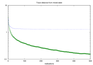
Figure 2: Trace distance between the average OBC-MPS with $\chi=2$ and the completely mixed state. The lower line is the trace distance between the average uniformely distributed random states and the completely mixed state.

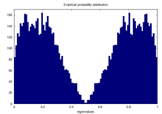
Figure 3: Empirical probability distribution for the eigenvalues of the reduced density matrix of RMPS (5000 states). The subsystem has dimension 2 and the total system has dimension 16 ($\chi=2$).

IV numerical results

The recent new approach to typicality comes in two main flavors, one due to Popescu et. al. PoShWi and a second one due to Reimann Rei1 . The first approach is more mathematical in two aspects: it uses results from the concentration of measure phenomenon and considers distances between states of subsystems. Reimann, on the other hand, uses more heuristic arguments and studies general observables. In this latter approach one has to show that the variance of the expectation values of observables is small and decreasing with the size of the bath. This implies, by the Chebyshev inequality, a concentration of measure result. With the approach of PoShWi one can directly study the fluctuations of the trace distance between the states in the ensemble and their average. A concentration result with this approach is a stronger result, in the sense that it is sufficient for having typicality at the level of observables. On the other hand typicality for all local observables can also imply a weaker concentration result for the state of the subsystem (see appendix C). In the numerical simulations we considered both the variance of the expectation value of observables and the fluctuations in the subsystem of the distance of RMPS from their average state $\overline{\rho}\equiv\overline{|\psi\rangle\langle\psi|}$, for which an exact expression can be obtained and reads in terms of the components

$$\overline{\rho_{{\bf\mathbf{i}},{\bf\mathbf{j}}}}={\rm Tr}_{\mathcal{H}_{A\otimes B}^{\otimes 2N}}\left[\left(|{\bf\mathbf{0}},{\bf\mathbf{j}}\rangle\langle{\bf\mathbf{i}},{\bf\mathbf{0}}|\otimes T\otimes T^{\dagger}\right)\overline{U^{\otimes N}\otimes U^{\dagger\otimes N}}\right],$$

where the $N-$components vectors are defined by ${\bf\mathbf{0}}\equiv(0,...,0),$ ${\bf\mathbf{i}}\equiv(i_{1},\dots,i_{N})$ and the same for ${\bf\mathbf{j}}.$ The operator $T$ acts on the $N-$tensor product of the ancilla system and cyclicly permutes the components

$$T|\alpha\rangle_{1}\dots|\alpha\rangle_{N}=|\alpha\rangle_{N}|\alpha\rangle_{1}\dots|\alpha\rangle_{N-1}.$$

The unitary random matrix $U(\chi D)$ is the one used in the sequential generation of the random MPS. A closed form for the average of the tensor product of unitaries $\overline{U^{\otimes N}\otimes U^{\dagger\otimes N}}$ is known CoSn . In Fig.2 we plot the trace distance between the average random MPS with OBC and the completely mixed state (for a chain of $4$ qubits) $\|\overline{\rho}-\frac{\mathbb{I}}{16}\|_{1}$, as a function of the size of the sampling set (the number of randomly generated states). In the same figure we also plot the same quantity in the case of random general pure state (not necessarily MPS). As can be seen from the figure the average OBC-RMPS is at a finite distance from the mixed state, while the average general state approaches the mixed state increasing the number of sampled states. Another distinctive feature of the homogeneous OBC-RMPS is shown in Fig.3, where we plot the empirical probability distribution of the eigenvalues of the reduced density matrix of 1 qubit in a 4-sites RMPS. In Fig.4 we show the same plot for general randomly generated states. As can be seen the two distribution differs significantly. From now on, unless otherwise stated, for all simulations we consider an ensemble of $500$ RMPS which originate from random unitaries distributed according to the Haar measure. We now want to illustrate our analytical results studying the behavior of the variance of $\sigma_{x}$, which acts on a particle ($L=1$) in the middle of the chain. Note that the important variable is not the absolute size of the subsystem or the bath but the ratio between them. As can be seen in Fig.5.a, when we fix the value of $\chi$ and increase the number of qubits in the bath the variance starts to decrease, but soon reaches a limiting value and does not decrease any more. The limiting value depends on $\chi$, becoming smaller as $\chi$ is increased. This could be expected from our bound and from a known property of MPS: correlations between system and environment are of finite range and depend on $\chi$. This is also consisten with recent result on finite entanglement scaling at criticality PoMuTu . Note, however, that our analytical result does not exclude the possibility of having typicality for fixed $\chi$ or $\chi$ scaling linearly with $N$. It only guarantees typicality in the case of a scaling greater than quadratic. We then analyze the case where $\chi=N-L$, as show in Fig.5.b. There it can be seen that until $\chi=N-L=180$ the variance is decreasing monotonically, which indicates that typicality can emerge already for a linear scaling of $\chi$ with the number of particles. However, at the present moment our simulations do not allow for a conclusive statement about the precise scaling of $\chi$ with $N-L$ that assures typicality.

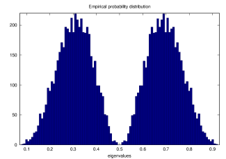
Figure 4: Empirical probability distribution for the eigenvalues of the reduced density matrix of a general Haar-distributed random state (5000 realizations). The subsystem has dimension 2 and the total system has dimension 16.

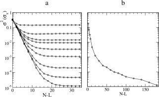
Figure 5: (a) The variance of the expectation value of $\sigma_{x}$ ($L=1$) increasing the size of the system and for fixed but different values of $\chi=2,4,6,8,12,20,50,100,\;\text{and}\;180$ (from top to bottom). (b) The variance of the expectation value of $\sigma_{x}$ ($L=1$) for increasing system size when the MPS dimension increases linearly with the number of particles in the bath: $\chi=N-L$.

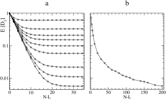
Figure 6: (a) The average trace distance from the average state of the ensemble of RMPS as the number of qubits in the environment ($N-L$) increases, for fixed but different values of $\chi=2,4,6,8,12,20,50,100,\;\text{and}\;200$ (from top to bottom) and for $L=1$. (b) The average trace distance from the average state of the ensemble of RMPS as the number of qubits in the environment ($N-L$) increases, taking the MPS dimension to increase linearly with the number of particles in the bath: $\chi=N-L$.

We also investigate the behavior of the average trace distance from the average state at the level of the sub-system, which is one particle in our case. Denoting with $\rho_{s}$ the reduced density matrix of the subsystem of a RMPS and $\overline{\rho_{s}}$ the average MPS, Fig.(6.a) shows the dependence on the size of the bath of the average value $E(D_{1})$ of the trace distance $D_{1}\equiv\|\rho_{s}-\overline{\rho_{s}}\|_{1}$. In general, we expect that having typicality at the level of states is harder than at the level of observables (see appendix C). Again we look at the case of fixed $\chi$ (Fig.(6.a)) and $\chi=N-L$ (Fig.(6.b)). The conclusions are similar to the case of observables, and it appears that even at the level of states typicality may occur already for a linear scaling of $\chi$ in the size of the bath, while the behavior for different but fixed values of $\chi$ is again consistent with well-known MPS properties.

V conclusions

In summary, we have shown that typicality can arise not only for an exponentially big Hilbert space but also for a physically accessible smaller set of states: the Matrix Product States. More specifically, we showed analytically that typicality occurs for MPSs having $\chi$ scaling polynomially in the size of the system (with a power greater than 2). We then presented some numerical calculations which indicate that typicality may already emerge for a linear scaling of $\chi$ in the system size at the level of both observables and the states.

Our results provide further evidence that typicality may play a role in a better understanding of the foundations of statistical mechanics. Nonetheless, there are still some aspects that require a deeper analysis. For example, it would be interesting to have more information on the average state obtained from the present ensemble of RMPS (in general $\overline{\rho}$ will still be a matrix product state but with a bigger rank than its components) and to better characterize the role of the geometry of the partition in between subsystem and bath and their correlations.

APPENDIX A. If $f$ is a real-valued function on a metric space $(X,d)$, its Lipschitz constant is

$$|f|_{\mathcal{L}}=sup_{x\neq y}\frac{|f(x)-f(y)|}{d(x,y)},$$

for $x,y\in X$. If $X=\mathbb{R}^{n},$ we let $d(x,y)=\|x-y\|,$ with

$$\|x\|=\left(\sum_{i=1}^{N}x_{i}^{2}\right)^{\frac{1}{2}}$$

the euclidean norm. The above notation can be easily applied also to the case when $X=\mathcal{M}_{n}(\mathbb{C})$ is the set of $n\times n$ matrices. For $A\in\mathcal{M}_{n}(\mathbb{C})$ we define

$$\|A\|_{\infty}=sup_{|\psi\rangle}\frac{\|A|\psi\rangle\|}{\||\psi\rangle\|},$$

$$\|A\|_{2}=\sqrt{Tr(A^{\dagger}A)},$$

$$\|A\|_{1}=Tr|A|.$$

All this norms are unitarily invariant and submultiplicative. In this work we used also the following relation

$$Tr(AB)\leq\|A\|_{\infty}\|B\|_{1}.$$

In the derivation of the upper bound for the Lipschitz constant we made use of standard properties of differentiation with respect to a matrix (MaNe )

$$dTr(X)=Tr(dX),$$

$$d(XY)=(dX)Y+X(dY),$$

where $X$ and $Y$ are arbitrary matrices. Defining the differential $df(X)$ to be the part of $f(X+dX)-f(X)$ which is linear in $dX$, the gradient $\nabla f$ satisfies $df=\nabla f\cdot dX$. Since the Lipschitz constant is equivalent to the $sup|\nabla f|,$ an upper-bound for the gradient will provide an upper-bound for the Lipschitz constant.

APPENDIX B. Here we review some of the notation used in the literature on MPS. A detailed exposition can be found in Verstraete08 . For brevity we will focus for the moment on normalized MPS with periodic boundary conditions, which by definition is a state that can be written as

$$|\psi\rangle=\sum_{i_{1},\dots,i_{N}=1}^{D}Tr(A^{i_{1}}[1]A^{i_{2}}[2]\dots A^{i_{N}}[N])|i_{1}i_{2}\dots i_{N}\rangle,$$

where the matrices $A$ are $\chi\times\chi$ complex matrices, labeled by the site index $\in\{1,\dots,N\}$ and by the local bases index $\in\{1,\dots,D\}.$

The expectation value of some operator $S,$ which is the tensor product of local operators $S[k]$ at each site $k$

$$S=S[1]\otimes\dots\otimes S[N],$$

is given by $\langle\psi|\bigotimes_{k=1}^{N}S[k]|\psi\rangle$ which is equal to

$$\sum_{i_{1},i_{1}^{\prime}\dots,i_{N},i_{N}^{\prime}}^{D}Tr\left(\prod_{k=1}^{N}A^{i_{k}}[k]\right)Tr\left(\prod_{k=1}^{N}A^{i_{k}^{\prime}}[k]^{*}\right)$$

$$\times\prod_{k=1}^{N}\langle i_{k}^{\prime}|S[k]|i_{k}\rangle$$

$$=\sum_{i_{1},i_{1}^{\prime}\dots,i_{N},i_{N}^{\prime}}^{D}Tr\left(\prod_{k=1}^{N}A^{i_{k}}[k]\otimes\prod_{k=1}^{N}A^{i_{k}^{\prime}}[k]^{*}\right)$$

$$\times\prod_{k=1}^{N}\langle i_{k}^{\prime}|S[k]|i_{k}\rangle$$

$$=\sum_{i_{1},i_{1}^{\prime}\dots,i_{N},i_{N}^{\prime}}^{D}Tr\left[\prod_{k=1}^{N}\left(A^{i_{k}}[k]\otimes A^{i_{k}^{\prime}}[k]^{*}\right)\right]\prod_{k=1}^{N}\langle i_{k}^{\prime}|S[k]|i_{k}\rangle$$

$$=Tr\left[\sum_{i_{1},i_{1}^{\prime}\dots,i_{N},i_{N}^{\prime}}^{D}\prod_{k=1}^{N}\langle i_{k}^{\prime}|S[k]|i_{k}\rangle\left(A^{i_{k}}[k]\otimes A^{i_{k}^{\prime}}[k]^{*}\right)\right]$$

$$=Tr\left[\prod_{k=1}^{N}\sum_{i_{k},i_{k}^{\prime}}^{D}\langle i_{k}^{\prime}|S[k]|i_{k}\rangle\left(A^{i_{k}}[k]\otimes A^{i_{k}^{\prime}}[k]^{*}\right)\right].$$

Defining the transfer matrix or transfer operator

$$E_{S[k]}[k]\equiv\sum_{i_{k},i_{k}^{\prime}}^{D}\langle i_{k}^{\prime}|S[k]|i_{k}\rangle\left(A^{i_{k}}[k]\otimes A^{i_{k}^{\prime}}[k]^{*}\right),$$

we see that

$$\langle\psi|\bigotimes_{k=1}^{N}S[k]|\psi\rangle=Tr\left[\prod_{k=1}^{N}E_{S[k]}[k]\right].$$

The normalization of the state is given by

$$Tr(\prod_{k=1}^{N}E_{\mathbb{I}[k]}[k]),$$ (6)

with $S[k]=\mathbb{I}[k]$ for all $k.$

Let us now consider the case of sequentially generated OBC-MPS ScHaWo . Consider a spin chain initially in a product state

$$|0\rangle^{\otimes N}\in\mathcal{H}_{B}^{\otimes N},$$

and an ancillary system initially in the state $|\phi_{I}\rangle\in\mathcal{H}_{A}.$ Let us introduce a unitary operator $U[k]$ acting on $\mathcal{H}_{A}\otimes\mathcal{H}_{B}$, for each site $k$ in the chain. Defining

$$A_{\alpha,\beta}^{i}[k]\equiv\langle i,\alpha|U[k]|\beta,0\rangle,$$

unitarity implies the following

$$U[k]^{\dagger}U[k]=\mathbb{I}_{D\chi}\implies\sum_{i}A^{i}[k]^{\dagger}A^{i}[k]=\mathbb{I}_{\chi}\quad k\in\{1,\dots,N\}.$$ (7)

Letting the ancilla interact sequentially with all the sites in the chain (see Fig.1) we obtain the state

$$|\psi\rangle=\sum_{i_{1},\dots,i_{N}=1}^{D}\langle\phi_{F}|A^{i_{N}}[1]\dots A^{i_{1}}[N]|\phi_{I}\rangle|i_{N}\dots i_{1}\rangle.$$

Let us write the OBC-MPS in a different way ($A^{i_{N+1}}[N+1]\equiv\langle\phi_{F}|$ and $A^{i_{0}}[0]\equiv|\phi_{I}\rangle$)

$$|\psi\rangle=\sum_{i_{1},\dots,i_{N}=1}^{D}A^{i_{N+1}}[N+1]A^{i_{N}}[1]\times$$

$$\times A^{i_{1}}[N]A^{i_{0}}[0]|i_{N+1}i_{N}\dots i_{1}i_{0}\rangle,$$

where $A^{i_{k}}[k]$ are $D_{k+1}\times D_{k}$ matrices with $D_{0}=D_{N+1}=1$ and $D_{k}=\chi$ with $k\in\{1,\dots,N\}$. The normalization of the MPS is given by

$$\langle\psi|\psi\rangle=\sum_{i_{0},\dots,i_{N+1}=1}^{D}A^{i_{0}}[0]^{\dagger}A^{i_{1}}[1]^{\dagger}\dots A^{i_{N+1}}[N+1]^{\dagger}\times$$

$$\times A^{i_{N+1}}[N+1]A^{i_{N}}[N]\dots A^{i_{1}}[1]A^{i_{0}}[0].$$

Using a singular value decomposition PeVeWo it is always possible to find a canonical form for $|\psi\rangle$ such that

$$\sum_{i_{N+1}}A^{i_{N+1}}[N+1]^{\dagger}A^{i_{N+1}}[N+1]=\mathbb{I}_{\chi}.$$

Using (7) recursively one has

$$\langle\psi|\psi\rangle=\sum_{i_{0}}A^{i_{0}}[0]^{\dagger}A^{i_{0}}[0]=1,$$

where the last equality follows from a normalization condition which can be imposed without loss of generality on the boundary local matrix $A^{i}[0]$ PeVeWo .

In the case of periodic boundary conditions the norm of the state

$$|\psi\rangle=\sum_{i_{1},\dots,i_{N}=1}^{D}Tr(A^{i_{1}}[1]A^{i_{2}}[2]\dots A^{i_{N}}[N])|i_{1}i_{2}\dots i_{N}\rangle,$$

is given by Eq.6 with $E_{\mathbb{I}}[k]\equiv\sum_{i_{k}=1}^{D}A^{i_{k}}[k]\otimes A^{i_{k}}[k]^{*}.$ For simplicity of notation, but without loss of generality, we shall restrict now to the translational invariant case. To any MPS it can always be associated a Completely Positive (CP) map PeVeWo

$$\mathcal{E}(X)\equiv\sum_{i}A_{i}XA_{i}^{\dagger}.$$

The CP map can always be assumed to have spectral radius 1 (corresponding to the absolute value of its maximum singular value) PeVeWo . The map $\mathcal{E}$ and $E_{\mathbb{I}}$ have the same spectrum since

$$\langle\beta_{1}|\mathcal{E}\left(|\alpha_{1}\rangle\langle\alpha_{2}|\right)|\beta_{2}\rangle=\langle\beta_{1},\beta_{2}|E_{\mathbb{I}}|\alpha_{1},\alpha_{2}\rangle.$$

Assuming that $\mathcal{E}$ has only one eigenvalue equal to 1 (without loss of generality PeVeWo ), one see that for $N$ big enough

$$\langle\psi|\psi\rangle=Tr\left(\prod_{k=1}^{N}E_{\mathbb{I}}\right)\approx\lambda_{1}^{N}=1,$$

where $\lambda_{1}$is the maximum eigenvalue equal to $1$. The corrections are exponentially suppressed in $N$. In our analytic derivation of an upper bound for the Lypschtiz constant of the function

$$f\equiv\frac{\langle\psi|\bigotimes_{k=1}^{N}S[k]|\psi\rangle}{\langle\psi|\psi\rangle}=\frac{Tr(\prod_{k=1}^{N}E_{S[k]}[k])}{Tr\left(\prod_{k=1}^{N}E_{\mathbb{I}}\right)},$$

we assume $N$ to be big enough that for all purposes

$$f=Tr(\prod_{k=1}^{N}E_{S[k]}[k]),$$

without the need of any additional normalization (and numerically this is verified to be true already for $N\geq 4$).

APPENDIX C. A concentration of measure result obtained for the trace distance between random states and their average implies the same concentration of measure result for the expectation values. This can be proved using the following general relation between the trace distance of normalized states and the difference between the expectation values of an observable $A$

$$|Tr(\rho A)-Tr(\psi A)|=|Tr(\rho-\psi)A|\leq\|\rho-\psi\|_{1}\|A\|_{\infty},$$

and we assume the operator norm of $A$ finite. If $\rho$ is a random state and $\psi$ is its average, one can see that a bound on the fluctuations of the right hand side of the above inequality implies a bound on the fluctuations of the left hand side. In general one can say that close states will have close expectation values for any observable of finite operator norm. But in general the converse is not true: if the expectation value of some observable with respect to different states is close this does not imply that the states are close. A way to estimate the state-distance is shown in PoShWi .

We prove in this manuscript that for the expectation value $f$ of any local observable, restricted to a subsystem of size $L$ much smaller than the size $N$ of the total system, the following holds true

$$Pr[|f-\overline{f}|>\epsilon]<c_{1}exp(-c_{2}^{\prime}\epsilon^{2}\chi/N^{2}),$$

where the sampling is done with respect to a set of random matrix product states of rank $\chi.$ Without lack of generality lets restrict to a chain of qubits. Any operator in the subsystem of size $L$ can be expressed in a basis of $4^{L}$ unitary orthogonal operators (for an explicit construction see PoShWi ). Lets call each element in this basis $U_{x},$ with $x\in\{1,\dots,4^{L}\}.$ We shall indicate with $\rho$ a realization of a normalized random matrix product state and with $\overline{\rho}$ the average state. Lets define $p_{x}(\rho)\equiv Tr(U_{x}\rho)$ and $p_{x}(\overline{\rho})\equiv Tr(U_{x}\overline{\rho})$. The previous concentration result holds true in particular for $p_{x}$ (for any $x$)

$$Pr[|p_{x}(\rho)-p_{x}(\overline{\rho})|>\epsilon]<c_{1}exp(-c_{2}^{\prime}\epsilon^{2}\chi/N^{2}).$$

Since there are $4^{L}$ different $x$ values we can also writhe

$$Pr[\exists x:|p_{x}(\rho)-p_{x}(\overline{\rho})|>\epsilon]<4^{L}c_{1}exp(-c_{2}^{\prime}\epsilon^{2}\chi/N^{2}).$$

Any random density matrix associated to the normalized RMPS can be written as $\rho=\sum_{x}p_{x}(\rho)U_{x}$. When $|p_{x}(\rho)-p_{x}(\overline{\rho})|<\epsilon$ for all $x$, then it follows

$$\|\rho-\overline{\rho}\|_{2}^{2} =\|\sum_{x}(p_{x}(\rho)-p_{x}(\overline{\rho}))U_{x}\|_{2}^{2}$$

$$= Tr\left[\sum_{x}\left(p_{x}(\rho)-p_{x}(\overline{\rho})\right)U_{x}\right]^{2}$$

$$= 4^{L}\sum_{x}\left(p_{x}(\rho)-p_{x}(\overline{\rho})\right)^{2}<4^{2L}\epsilon^{2}.$$

We can write then

$$\|\rho-\overline{\rho}\|_{1}\leq\sqrt{4^{L}}\|\rho-\overline{\rho}\|_{2}<4^{3L/2}\epsilon$$

and from this it follows

$$Pr[\|\rho-\overline{\rho}\|_{1}>4^{3L/2}\epsilon]<4^{L}c_{1}exp(-c_{2}^{\prime}\epsilon^{2}\chi/N^{2}).$$

Which tells us that keeping $L$ fixed and much smaller than $N$, for $\chi\propto N^{3}$and $\epsilon\propto N^{-1/3}$one has

$$Pr[\|\rho-\overline{\rho}\|_{1}>4^{3L/2}N^{-1/3}]<4^{L}exp(-N^{1/3}).$$

This prove a concentration of measure result “at the level of states”. But this result is weaker with respect to the result for the observables by a factor $4^{L}$.

References

(1) J. Gemmer, M. Michel and G. Mahler, Lecture Notes
in Physics 657, Springer-Verlag (2004).
(2) J.L. Lebowitz, arXiv:cond-mat/9605183.
(3) S. Goldstein, J. L. Lebowitz, R. Tumulka and N.
Zanghi, Phys. Rev. Lett. 96, 050403 (2006).
(4) S. Popescu, A. Short and A. Winter, Nature Physics
2, 754 (2006).
(5) P. Reimann, Phys. Rev. Lett. 99, 160404 (2007).
(6) P. Reimann, Phys. Rev. Lett. 101, 190403
(2008).
(7) J.Emerson, Y.S.Weinstein,M.Saraceno,S.Lloyd and
D.C. Cory, Science 302, 2098 (2003).
(8) M.Rigol, V.Dunjko and M.Olshanii, Nature (London)
452, 854 (2008).
(9) S. R. White, Phys. Rev. Lett. 102, 190601
(2009)
(10) E.Schrodinger, Annalen der Physik (4), 83
(1927).
(11) F. Verstraete, J.I. Cirac, V. Murg, Adv. Phys.
57, 143 (2008).
(12) M. B. Hastings, Phys. Rev. A 76, 032315 (2007).
(13) D. Perez-Garcia, F. Verstraete, M.M. Wolf and J.I.
Cirac, Quantum Inf. Comput. 7, 401 (2007).
(14)G. Vidal, Phys. Rev. Lett 91, 147902 (2003).
(15) C. Schon, K. Hammerer, M.M Wolf, J.I. Cirac and
E. Solano, Phys. Rev. A 75, 032311 (2007).
(16) V. D. Milman and G. Schechtman, Asymptotic
theory of finite dimensional normed spaces, Number 1200 in Lecture
Notes in Mathematics, Springer-Verlag, 1986.
(17) P.Hayden, D.Leung,P. W. Shor and A. Winter, Comm.
Math. Phys. 2, 371 (2004).
(18) D. Gross, S. T. Flammia, and J. Eisert, Phys. Rev.
Lett. 102, 190501 (2009).
(19) M. J. Bremner, C. Mora, and A. Winter, Phys. Rev.
Lett. 102, 190502 (2009).
(20) R. A. Low, arXiv:0903.5236v1.
(21) B. Collins, P. Sniady, Commun. Math. Phys. 264,
773 (2006).
(22)F. Pollmann, S. Mukerjee, A. M. Turner, and J. E.
Moore, Phys. Rev. Lett. 102, 255701 (2009).
(23) J. R. Magnus and H. Neudecker, Matrix differential
calculus with applications in statistics and econometrics, John Wiley
& Sons, 1988.