Shirley Interpolation - Optimal basis sets for detailed Brillouin zone integrations revisited

Abstract

We present a new implementation of the k-space interpolation scheme for electronic structure presented by E. L. Shirley, Phys. Rev. B 54, 16464 (1996). The method permits the construction of a compact k-dependent Hamiltonian using a numerically optimal basis derived from a coarse-grained set of effective single-particle electronic structure calculations (based on density functional theory in this work). We provide some generalizations of the initial approach which reduce the number of required initial electronic structure calculations, enabling accurate interpolation over the entire Brillouin zone based on calculations at the zone-center only for large systems. We also generalize the representation of non-local Hamiltonians, leading to a more efficient implementation which permits the use of both norm-conserving and ultrasoft pseudopotentials in the input calculations. Numerically interpolated electronic eigenvalues with accuracy that is within 0.01 eV can be produced at very little computational cost. Furthermore, accurate eigenfunctions - expressed in the optimal basis - provide easy access to useful matrix elements for simulating spectroscopy and we provide details for computing optical transition amplitudes. The approach is also applicable to other theoretical frameworks such as the Dyson equation for quasiparticle excitations or the Bethe-Salpeter equation for optical responses.

I introduction

Providing efficient access to accurate electronic structure is vital to accelerating research in materials science and condensed matter physics. This can be achieved directly by increasing the availablility of computational resources, by developing faster numerical methods, or by switching to more compact numerical representations. However, if one adheres to existing methods and representations, one might reasonably ask if more information can be extracted efficiently from such approaches. In this work, we outline an efficient approach to extracting detailed information on electronic structure for arbitrary electron wave vector $\mathbf{k}$. This method applies not only to periodic systems – where $\mathbf{k}$ is well-defined – but also to models of aperiodic systems within the supercell approach (COHEN et al., 1975). For example, periodic calculations are often used to simulate isolated molecules in large supercells and disordered condensed phases are commonly modeled using a supercell of sufficient size to contain relevant structural features. Providing efficient access to first principles electronic band structure and matrix elements over the entire Brillouin zone (BZ) supports a wide range of research topics from Fermi surface exploration in superconducting materials to detailed simulated spectroscopy of dispersive bands or high energy excitations.

In 1996, Shirley (Shirley, 1996) outlined an approach within effective single-particle electronic structure for constructing an optimal basis which spans the BZ and can be used to build a compact k-dependent Hamiltonian based on some coarse-grained reference calculations. He applied this approach in detailed explorations of the dispersion and spectroscopy of crystalline systems: silicon, germanium, graphite, hexagonal boron nitride, lithium fluoride, and calcium fluoride. The efficacy of his approach was tested by examination of electron band structures, densities of states, dielectric properties, x-ray resonance fluorescence and incoherent emission spectra, and photoelectron spectroscopy, with details provided or referenced in (Shirley, 1996). He also used this basis in developing efficient approaches to Bethe-Salpeter calculations for valence-band (Benedict et al., 1998) and core-level spectroscopy (Shirley, 1998). To our knowledge, this advantageous approach has not been widely applied outside of Shirley’s research. In this work, we outline a generalized implementation of Shirley’s interpolation scheme, which has been incorporated as a post-processing tool for use with the Quantum-ESPRESSO (Giannozzi et al., 2009) open-source electronic structure package. We hope that the outline provided here indicates how easily Shirley interpolation might be implemented in other electronic structure codes. Furthermore, we illustrate that the advantages of such an approach are clear when applied to large supercell calculations, where zone-center electronic structure calculations are sufficient to accurately reproduce the electronic structure throughout the BZ. This particular implementation has already been used in simulating x-ray absorption spectra of molecules in vacuo (Uejio et al., 2008; Schwartz et al., 2009a)and in solution (Schwartz et al., 2009b).

Another commonly used interpolation scheme for electronic structure exploits maximally localized Wannier functions(Mostofi et al., 2008). This approach builds a set of Wannier functions to describe a band complex and minimizes their spread in real-space. The resulting functions can be quite localized and enable the calculation of first-principles tight-binding parameters for use in calculations of Berry’s phase polarization(Souza et al., 2000; Stengel and Spaldin, 2006), electron transport(Calzolari et al., 2004), electron-phonon coupling(Giustino et al., 2007a, b), and much more. The Shirley interpolation method does not produce spatially localized functions. However, for interpolation purposes, we show that it is much more automatic to use and computationally less expensive in terms of required input calculations. Also, conduction band states may be generated as easily as valence band states. In particular, there are no intrinsic difficulties in treating metallic systems and no specific requirements for disentanglement of dispersive bands(Souza et al., 2002).

This paper is organized as follows: In Section II we provide a summary of the work outlined in Ref. Shirley, 1996. In Section III and IV we focus on the advances in our particular implementation over the original work. Section V focuses on some applications which highlight the advantages of the approach. Section VI differentiates Shirley interpolation from Wannier interpolation. Finally, in Section VII we provide some potential applications of this approach and then summarize our conclusions in Section VIII.

II Background to the Method

Figure 1: The steps involved in building the compact k-dependent Hamiltonian in the optimal basis, beginning (top) with a self-consistent charge density, from which states are generated for a range of bands and k-points. An overlap matrix is constructed from the periodic parts of these Bloch states and diagonalized. The optimal basis is chosen as those eigenvectors of the overlap matrix (ordered by eigenvalue magnitude) which span a user-defined fraction of the space defined by the input states. The k-dependent Hamiltonian is constructed in this basis from its various parts: kinetic energy, local potential, and non-local potential.

A brief summary of Shirley’s approach is provided here to establish the context of our own work. The process of building a compact k-dependent Hamiltonian in the optimal basis for Brillouin zone sampling is outlined in Figure 1. We assume an effective single-particle Hamiltonian (based on Kohn-Sham density functional theory(Hohenberg and Kohn, 1964; Kohn and Sham, 1965) in this work). A self-consistent charge density is generated by sufficient sampling of the Brillouin zone. Then, if necessary, a set of states is calculated from this density for a user-specified set of band indices and k-points. The periodic parts of these Bloch-states are extracted and used to construct an overlap matrix which is then diagonalized to isolate linear dependence in this basis of periodic functions. By ordering the overlap eigenvalues by decreasing magnitude, we may select the optimal basis subject to a user-defined tolerance. In our approach we truncate the basis by specifying a tolerance $\epsilon$ for the neglected fraction of the trace of the overlap.

Since we have removed the plane-wave envelope functions from the Bloch-states, a k-dependent Hamiltonian is required, and we represent this Hamiltonian $H(\mathbf{k})$ in the optimal basis. Each component of the Hamiltonian is expanded as a polynomial in $\mathbf{k}$. The kinetic energy has an analytic quadratic form, as indicated in Fig. 1. Specifically, with access to the Fourier coefficients of the optimal basis functions $B_{i}(\mathbf{G})$, if one expands the k-dependent kinetic energy operator, one obtains:

$$\langle B_{i}|e^{-i\mathbf{k\cdot r}}\left(-\frac{1}{2}\nabla^{2}\right)e^{i\mathbf{k\cdot r}}|B_{j}\rangle$$

$$= -\frac{1}{2}\left[k^{2}\delta_{ij}+\mathbf{k\cdot}\sum_{\mathbf{G}}B_{i}(\mathbf{G})^{*}\mathbf{G}B_{j}(\mathbf{G})\right.$$

$$\left.\hskip 30.00005pt+\sum_{\mathbf{G}}B_{i}(\mathbf{G})^{*}G^{2}B_{j}(\mathbf{G})\right]$$

$$\equiv -\frac{1}{2}\left[k^{2}\delta_{ij}+\mathbf{k\cdot}\mathbf{K}_{ij}^{(1)}+K_{ij}^{(0)}\right].$$

The local potential is constant with respect to $\mathbf{k}$ and its matrix elements are efficiently computed within a plane-wave code using Fast Fourier Transforms. The non-local potential requires fitting on a grid in k-space. In Shirley’s implementation (Shirley, 1996), k-dependent matrix elements of the non-local potential operator were evaluated at points on a uniform Cartesian grid which contained the entire first Brillouin zone and these were fitted to polynomials in $\mathbf{k}$ to enable interpolation between the points. Explicit expressions for each term in the Hamiltonian were provided in the original work.

The outcome of these steps is a set of coefficients which can be used to construct the matrix $H(\mathbf{k})$ for any $\mathbf{k}$ and then diagonalize it to produce the eigenvectors and eigenvalues in good agreement with an equivalent solution to the underlying Hamiltonian at the same k-point. The advantage of Shirley’s approach is that one reduces the size of the problem to be solved (i.e., the dimension of $H$) such that detailed explorations of the eigenspectrum become tractable. For instance, one could expect to switch from thousands of plane-waves to perhaps tens of optimal basis functions, thereby reducing a tough iterative (most likely parallelized) diagonalization to a trivial direct diagonalization which can be solved efficiently on a single processor. Shirley’s satisfaction with the efficacy of this approach is clear in his original paper and also from the large number of detailed spectroscopic simulations enabled by it.

III More efficient routes to the optimal basis

III.1 Choice of k-points for the optimal basis

The original scheme outlined particular uniform Cartesian grids in k-space at which eigensolutions were generated using the DFT code of choice and provided as input to construct the optimal basis by diagonalization of their overlap matrix. Henceforth, we shall refer to these DFT eigensolutions as “input states” and the k-space grid on which they are calculated as the “input grid”. In general, the “input grid” need not coincide with that used in the original self-consistent DFT calculation, which generated the self-consistent charge density, and the range of band indices for a given application may also differ, particularly when exploring the unoccupied spectrum. Therefore, the input states are often generated directly as solutions to the Kohn-Sham equations for a fixed self-consistent field. In the original work, the input grids contained the entire first Brillouin zone, with the aim of reproducing the eigensolutions at all points in that zone. It was not clear from the original work how the final accuracy would be affected by particular choices of such coarse input grids. Furthermore, the choice of input grid varied with lattice symmetry due to the differences in the shape of the first Brillouin zone in Cartesian space. In this work, we instead present a more general and automatic approach to sampling k-space based on uniform grids in reciprocal lattice space, spanning the unit cube $[0,1]^{3}$. This means that for any lattice symmetry, the input grid of k-points may be characterized uniquely by three integers $n_{1}\times n_{2}\times n_{3}$, much like a typical electronic structure calculation. Furthermore, one can be sure that this grid spans the volume of the Brillouin zone. In the original scheme, the use of a Cartesian input grid leads to the inclusion of some k-points lying outside the zone boundary for non-orthorhombic cells.

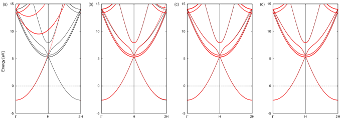
Figure 2: Accuracy in reproducing the band structure of bcc Na with respect to choice of input k-point grid. Band energies are reported in eV with respect to the Fermi level and k-points follow the $\Delta$ line from the zone center ($\Gamma$) to one of the zone boundaries ($H$) and beyond to a periodic image of the zone-center ($2H$). DFT (Shirley interpolated) band structure is indicated by black lines (red dots). The size of the input k-point grid is varied: (a) $\Gamma$ only; (b) $\Gamma$ and $H$; (c) $\Gamma$, $H$ and $2H$; (d) $\Gamma$ together with its seven periodic images from the corners of the unit cube $[0,1]^{3}$.

III.2 Building in periodicity with respect to $\mathbf{k}$

As stated by Shirley, the k-dependent Hamiltonian does not impose periodicity in k-space, and so, one must be careful regarding the k-points one passes to the Hamiltonian for diagonalization. We illustrate this point in Figure 2 by examining the band structure of bcc Na along the $\Delta$ line connecting the $\Gamma$ and $H$ points, with extension to the $2H$ point, which is equivalent to $\Gamma$. We chose Na since its electronic structure is well described at the DFT level using a local pseudopotential, thereby removing any complications associated with interpolating the non-local potential. In this calculation, we employed a norm-conserving pseudopotential and a 30 Ry kinetic energy cut-off. The interpolated band structure is clearly dependent on the choice of input k-points used to generate the basis. Using the $\Gamma$-point alone [Fig. 2(a)] results in accurate electronic bands at that point, but large errors as one follows the $\Delta$ line. Most notably, the periodic image of the zone-center, $2H$, is completely wrong, which emphasizes that we have no explicit periodic boundary condition in our k-dependent Hamiltonian. Inclusion of the zone-boundary $H$ point [Fig. 2(b)] leads to marked improvement in accuracy along $\Delta$ but leads to some inaccuracy once we leave the zone-centered first Brillouin zone – again the $2H$ point is not reproduced. However, the ability to obtain excellent agreement in band structure between the input grid points naturally prompts one to continue adding points to enable reproducibility over a larger region of k-space. Explicitly adding the $2H$ point [Fig. 2(c)] does indeed almost restore the correct symmetry of the band structure, albeit only in the neighborhood of this $[\Gamma,2H]$ interval – we should expect no reproducibility outside this interval. At this point, one can appreciate Shirley’s original Brillouin zone-spanning choice of input grids, as they guarantee accurate reproducibility of band structure throughout the zone. However, for cases where certain high-symmetry points are not included in the input grid, inaccuracies may appear.

We have observed that the input grid does not define a “fit” in the usual sense of interpolation, with reproducibility decreasing in accuracy as one explores points farther away (in the Cartesian sense) from the grid points. In fact, when we include the $H$ point, we notice that the entire $\Delta$ line is accurately reproduced. Furthermore, if we were to include $\Gamma$ and its periodic image $2H$ alone, we would see reasonable reproducibility across the entire $\Delta$ line. Clearly, it seems that there is sufficient k-dependence built into $H(\mathbf{k})$ to accurately describe the full-zone, once we provide additional constraints on the symmetry via the input states. This is equivalent to a phase-constraint for the optimal basis, as we shall see next section. And so, in our implementation we provide input grids chosen uniformly from the unit cube, including all corners of the cube. We furthermore impose periodicity on k-points requested for diagonalization by mapping them first to the unit cube (in reciprocal lattice coordinates), since we have no guarantee of accuracy outside the three-dimensional interval $[0,1]^{3}$.

III.3 Accurate interpolation using just the $\Gamma$-point

If we choose our input grid from the unit cube, it seems clear now that we should include all corners of the cube – $\Gamma$ and its seven periodic images in three dimensions. Always wanting to reduce computational effort, we immediately see that the input states originating from these periodic images differ only in phase from those at $\Gamma$. Furthermore, we will see that, for large supercells (small Brillouin zones), it is sufficient, using a DFT calculation, to generate input states at $\Gamma$ only, generating periodic images of these states at the corners of the unit cube in a small number of steps. Figure 2(d) illustrates how well this approach works for bcc Na. The resulting band structure is indistinguishable (by eye) from the original. The root-mean-square error along the indicated path is 5.5 meV. We may reduce this error by including more input k-points. However, we note that this error will not tend to zero, since it is comparable to the error associated with changing the kinetic energy cut-off and is related to a slight inconsistency in the number of plane-waves between periodic functions from different k-points (as noted by Shirley). In our implementation, we retain all wave vectors $\mathbf{G}$, such that $\frac{1}{2}|\mathbf{k}+\mathbf{G}|^{2}\leq E_{cut}$, padding with zeros the coefficients of those functions with missing $\mathbf{G}$. Note that numerical differences related to this effect reduce in magnitude for larger cut-offs, but in essence they are inconsequential, given that the original DFT calculated eigenvalues would change as much upon varying $E_{cut}$. Generally, for large supercells we find that $\Gamma$-point sampling is adequate to reproduce all of the band structure with an accuracy that is within 10 meV.

To reduce the cost of the input DFT calculation, we construct the periodic images of the input states. The transformation of a given periodic function $u_{n\mathbf{k}}$ to $u_{n\mathbf{k+G_{0}}}$ is easy to obtain in plane-wave representations. Since periodicity implies that

$$u_{n\mathbf{k}}(\mathbf{r})e^{i\mathbf{k.r}} = u_{n\mathbf{k+G_{0}}}(\mathbf{r})e^{i(\mathbf{k+G_{o}})\mathbf{.r}}$$

$$e^{-i\mathbf{G_{0}.r}}u_{n\mathbf{k}}(\mathbf{r}) = u_{n\mathbf{k+G_{0}}}(\mathbf{r})$$

then, expanding in Fourier coefficients, we have

$$\sum_{\mathbf{G}}c_{n\mathbf{k}}(\mathbf{G})e^{i(\mathbf{G-G_{0}})\mathbf{.r}} = \sum_{\mathbf{G}}c_{n\mathbf{k+G_{0}}}(\mathbf{G})e^{i\mathbf{G.r}},$$

which implies that the Fourier coefficients are ultimately reordered according to $c_{n\mathbf{k}}(\mathbf{G+G_{0}})=c_{n\mathbf{k+G_{0}}}(\mathbf{G})$.

For applications to large systems, where wave functions are necessarily distributed over many processors, such reordering may be complicated to implement. In this case, a simpler, albeit less efficient approach, is to exploit the native implementation of the Fourier transform to make such a transformation. Suppose that we start with the wave functions in Fourier space. Then we follow this map

$\begin{array}[]{ccc}c_{n\mathbf{k}}(\mathbf{G})&\rightarrow&u_{n\mathbf{k}}(\mathbf{r})\\ &&\downarrow\\ c_{n\mathbf{k+G_{0}}}(\mathbf{G})&\leftarrow&e^{-i\mathbf{G_{0}.r}}u_{n\mathbf{k}}(\mathbf{r})\end{array}$

where we first back-transform to real-space, then multiply by the function $e^{-i\mathbf{G_{o}.r}}$ for each $\mathbf{r}$, and then Fourier transform again to reciprocal space.

Note that for cases where the $\Gamma$-point alone is insufficient, this scheme could also be generalized to expand input states to the star of a given input k-point by employing the little-group of that k-point as determined by the lattice and atomic basis symmetry.

IV Generalization of the non-local potential

IV.1 Generalized Kleinman-Bylander form

At this point we choose an advantageous deviation from the original implementation (Shirley, 1996). The k-dependent non-local potential is arbitrarily complex with respect to ${\bf k}$. Previously, Shirley expanded the entire operator in the optimal basis on a coarse grid in k-space and then interpolated between these values using a polynomial expansion. This was probably the most complex component of the original approach with respect to implementation. Details were provided for a quartic interpolation based on a $5\times 5\times 5$ grid, however, the generalization to different grids and the relative importance of such effort was left to the judgement of the reader for specific examples. Storage of the ultimate parametrization of the non-local potential is proportional to the grid size and the square of the number of basis functions. In this work, we take a slightly different approach, which we will show to be more compact in many cases and more powerful in terms of deriving spectroscopic information.

We assume a generalized, separable, Kleinmann-Bylander (KLEINMAN and BYLANDER, 1982) form for the non-local potential

$$V^{NL} = \sum_{\lambda\lambda^{\prime}}|\beta_{\lambda}\rangle D_{\lambda\lambda^{\prime}}\langle\beta_{\lambda^{\prime}}|$$ (1)

This is most reminiscent of Vanderbilt’s ultrasoft pseudopotentials (VANDERBILT, 1990). Note that for norm-conserving pseudopotentials $D_{\lambda\lambda^{\prime}}$ is diagonal. The composite index $\lambda=(I,n,l,m)$ refers to the site $I$ of a particular ion and its associated atomic quantum numbers. Expanding the k-dependent version of this operator in the optimal basis, we find that the k-dependence is limited to the projectors

$$V_{ij}^{NL}(\mathbf{k\mathrm{)}} = \sum_{\lambda\lambda^{\prime}}\beta_{\lambda i}(\mathbf{k})^{*}D_{\lambda\lambda^{\prime}}\beta_{\lambda^{\prime}j}(\mathbf{k}),$$ (2)

where

$$\beta_{\lambda i}(\mathbf{k}) = \langle\beta_{\lambda}|e^{i\mathbf{k\cdot r}}|B_{i}\rangle.$$

So, we may consider interpolating only the projector matrix elements on a grid in k-space. The k-dependent projectors are quite efficiently evaluated by one-dimensional Fourier transform of their radial component and should be obtainable from the original electronic structure code. In order to make our implementation general, we employ three-dimensional B-spline interpolation (de Boor, 1978; Schadow, ) on a uniform $n_{1}\times n_{2}\times n_{3}$ grid of k-points in crystal coordinates, that is, chosen from the unit cube, $[0,1]^{3}$. Requests for evaluations of the non-local projectors at k-points outside the unit cube assume periodicity in k-space. In general, we use a larger k-point grid to interpolate the projectors than we use for generating the optimal basis. A good rule of thumb is to use a grid at least twice as dense. We note that for systems with $d$-electrons we have used more dense grids. We also avoid spurious interpolation by limiting the order of the B-splines to be equal to the number of grid points in each dimension. Note that for an $n_{1}\times n_{2}\times n_{3}$ grid, each dimension is actually expanded by one to include the edges of the unit cell.

Note that by interpolating the projectors, one must construct the full non-local potential for each $\mathbf{k}$ by matrix multiplication. This apparent additional cost is not that great, considering that for norm-conserving pseudopotentials $D_{\lambda\lambda^{\prime}}$ is diagonal, and even for ultrasoft pseudopotentials $D_{\lambda\lambda^{\prime}}$ is block-diagonal. This specific choice for interpolation can reduce the required storage for the non-local potential by the ratio of the number of projectors to the number of basis functions, which for many applications is a reduction on the order of hundreds, given that there may be typically 100 basis functions per atom, but likely less than 10 projectors.

IV.2 Extension to ultrasoft pseudopotentials

The extension of the original approach to ultrasoft pseudopotentials is now trivial. Ultrasoft pseudopotentials relax the norm-conservation condition, by introducing a correction derived from atomic all-electron and pseudo waves:

$$Q_{\lambda,\lambda^{\prime}}(\mathbf{r}) = \psi_{\lambda}(\mathbf{r})^{*}\psi_{\lambda^{\prime}}(\mathbf{r})-\phi_{\lambda}(\mathbf{r})^{*}\phi_{\lambda^{\prime}}(\mathbf{r})$$

$$Q_{\lambda,\lambda^{\prime}} = \langle\psi_{\lambda}|\psi_{\lambda^{\prime}}\rangle-\langle\phi_{\lambda}|\phi_{\lambda^{\prime}}\rangle$$

where $\psi,\phi$ refer to all-electron and pseudo waves respectively. This correction appears in the coefficients that define the non-local potential:

$$D_{\lambda,\lambda^{\prime}} = D_{\lambda,\lambda^{\prime}}^{ion}+D_{\lambda,\lambda^{\prime}}^{Hxc},$$

where the first term is a constant for each atomic species, while the second term involves an integral of $Q_{\lambda,\lambda^{\prime}}(\mathbf{r})$ over the density dependent Hartree plus exchange-correlation potential (VANDERBILT, 1990).

Furthermore, we must remember that the use of ultrasoft pseudopotentials introduces a generalized orthonormality condition on the eigensolutions

$$\langle n\mathbf{k}|S|m\mathbf{k}\rangle = \delta_{nm},$$

which implies that their periodic components are solutions to the following generalized eigen-problem:

$$[H(\mathbf{k})-\epsilon_{n\mathbf{k}}S(\mathbf{k})]|u_{n\mathbf{k}}\rangle = 0.$$

The k-dependent overlap matrix in the optimal basis is defined to be

$$S_{ij}(\mathbf{k}) = \sum_{\lambda,\lambda^{\prime}}\beta_{\lambda i}(\mathbf{k})^{*}Q_{\lambda,\lambda^{\prime}}\beta(\mathbf{k}),$$

and the projectors matrix elements $\beta_{\lambda i}(\mathbf{k})$ are identical with those used in the non-local potential. Note that this introduces a large storage and computational saving: we need only interpolate the projector matrix elements once, and then we can construct both the non-local potential and overlap matrix by multiplication.

In summary, the generalization to ultrasoft pseudopotentials has the following additional requirements for construction of the k-dependent Hamiltonian: (1) access to the self-consistent coefficients $D_{\lambda,\lambda^{\prime}}^{Hxc}$ at the end of the SCF calculation and (2) access to the $Q_{\lambda,\lambda^{\prime}}$ coefficients available in the pseudopotential definitions. Subsequently, at any k-point, one must find the solution of a generalized eigen-problem with both $H(\mathbf{k})$ and $S(\mathbf{k})$ constructed by interpolation.

IV.3 Advantages for spectroscopy

One of the most common matrix elements used for optical spectroscopy is that of the velocity operator. However, for non-local Hamiltonians, its evaluation is non-trivial, involving a commutator of the position operator and the non-local potential (STARACE, 1971; KOBE, 1979; HYBERTSEN and LOUIE, 1987; READ and NEEDS, 1991; Kageshima and Shiraishi, 1997). Several approaches have been introduced to include or overcome this complication. For instance, rather than evaluating matrix elements of velocity in the transverse gauge, one can equivalently evaluate plane-wave matrix elements in the longitudinal gauge, exploiting the Heisenberg equation of motion:

$$\langle n\mathbf{k}|\mathbf{\hat{q}\cdot v}|m\mathbf{k}\rangle = \lim_{q\rightarrow 0}\frac{[\epsilon_{m\mathbf{k}+\mathbf{q}}-\epsilon_{n\mathbf{k}}]}{q}\langle n\mathbf{k}|e^{-i\mathbf{q\cdot r}}|m\mathbf{k}+\mathbf{q}\rangle,$$

where $\mathbf{\hat{q}}$ is the polarization of the incident electric field. Substitution of the commutator $[e^{-iq\cdot r},H]$ in this expression leads to the following identity:

$$\langle n\mathbf{k}|\mathbf{\hat{q}\cdot v}|m\mathbf{k}\rangle = \lim_{q\rightarrow 0}\langle u_{n\mathbf{k}}|\frac{H(\mathbf{k}+\mathbf{q})-H(\mathbf{k})}{q}|u_{m\mathbf{k}+\mathbf{q}}\rangle$$

$$= \langle u_{n\mathbf{k}}|\hat{\mathbf{q}}\cdot\frac{dH(\mathbf{k})}{d\mathbf{k}}|u_{m\mathbf{k}}\rangle.$$

One advantage of our current implementation is the ability to evaluate derivatives of $H(\mathbf{k})$ with respect to $\mathbf{k}$. The kinetic energy operator is readily differentiable, while the B-spline routines we adopted also include efficient evaluation of derivatives (Schadow, ). Therefore, very little extra work is required to access optical transition amplitudes. Beyond first derivatives, one can see that accurate effective masses are easily attainable through the second derivatives and would be extremely efficient for large periodic nanostructures, obviating the need for numerical differentiation based on multiple costly k-point calculations.

V Applications

Previous work has shown the efficacy of Shirley interpolation in reproducing the band structure of crystalline solids. Instead, we choose to focus on supercells, where the efficiency of Shirley’s approach is clearly competitive with the usual plane-wave calculations, while retaining the accuracy of self-consistent results.

V.1 Large systems using only the $\Gamma$-point

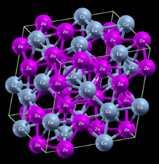
Figure 3: The atomic structure of $\gamma$-brass (Cu₅Zn₈)

We choose $\gamma$-brass ($\mbox{Cu}_{5}\mbox{Zn}_{8}$) as an example of a crystalline solid with a large unit cell containing 26 atoms (Fig. 3). We generate the self-consistent field using a shifted $4\times 4\times 4$ k-point grid within DFT using ultrasoft pseudopotentials for Cu and Zn, a plane-wave cut-off of 25 Ry and a charge density cut-off of 200 Ry. The basis is built using 200 input states calculated at the $\Gamma$-point, which are then expanded to include the seven images of the $\Gamma$-point at the corners of the reciprocal space unit cube. The optimal basis is obtained by diagonalizing the overlap matrix and truncating to 1095 functions from a possible 1600, corresponding to $\sim 42$ basis functions per atom. The non-local potential is interpolated on a $3\times 3\times 3$ grid. The non-dispersive $d$-bands of Cu and Zn require this level sampling in order to accurately reproduce the non-local potential. The resulting band structure is shown in Figure 4. Comparison with DFT calculations throughout the Brillouin zone indicates remarkable accuracy (root-mean-square deviation of 2 meV) for the interpolated band structure, with all bands of all character ($s,p,d$) reproduced to the same degree. We can efficiently refine a non-self-consistent estimate of the Fermi-level using Shirley interpolation, and we find it to be shifted from that of our initial self-consistent-field plane-wave calculation by 0.3 eV. This is a good illustration of the importance of detailed k-point sampling in metals. Shirley interpolation provides an efficient route to obtaining a more accurate estimate of the Fermi level for a given self-consistent field and indicates the possibility of using this interpolation scheme to efficiently refine self-consistent-field calculations for metallic systems.

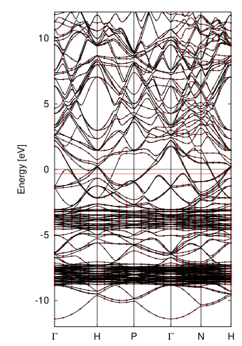
Figure 4: The electron band structure of $\gamma$-brass (Cu₅Zn₈) generated using plane-wave DFT calculations (red dots) and using Shirley interpolation based solely on DFT wave functions generated at the $\Gamma$-point (black lines). The root-mean-square deviation of the Shirley interpolated values is 2 meV. The black (red) horizontal line indicates the Fermi level resulting from a $4\times 4\times 4$ k-point plane-wave DFT calculation ($10\times 10\times 10$ k-point Shirley interpolation).

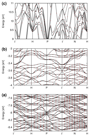
Figure 5: Details of the band structure of $\gamma$-brass in three energy regions: (a) the Zn $d$-bands; (b) the Cu $d$-bands; and (c) high in the conduction bands. DFT plane-wave calculations are indicated by red dots. Shirley interpolated bands are shown as black lines. Together with Fig. 4 this indicates the ability of Shirley interpolation to accurately reproduce the bands of metallic states of varying character with minimal effort ($\Gamma$-point calculations only).

V.2 Efficiency in vacuo

When using plane-waves in supercell simulations of reduced dimensional systems, the inclusion of large vacuum regions comes at a significant computational cost. The use of Shirley interpolation can reduce this cost dramatically. We use graphene as an example, where we simulate this two-dimensional sheet of carbon atoms in a three-dimensional supercell with a large separation between periodic images defined by the $c$-axis. We notice that increasing $c$ results in a large increase in the number of plane-waves in this dimension, but has only a small impact on the number of optimal basis functions used to construct the Shirley Hamiltonian. Table 1 clearly illustrates the efficiency of the Shirley approach for k-point sampling. In this small example we see speed-ups of greater than 3000. Furthermore, the increase in computational effort that we expect when adding to the vacuum spacing is practically absent from the interpolated case where the number of basis functions increase only slightly, rather than the linear increase for plane-waves.

$c$	$N_{PW}$	$T_{PW}$	$M{}_{S}$	$T{}_{S}$
$\AA$		s		s
10	21993	191.56	244	0.063
15	32971	220.48	255	0.056
20	43975	234.88	279	0.056

Table 1: Timing information per k-point calculation for graphene supercells of varying planar separation $c$, when using a plane-wave DFT code $T_{PW}$ with a basis of $N_{PW}$ plane-waves, and when using Shirley interpolation $T_{S}$, with $M_{S}$ basis functions.

VI Comparison with Wannier Interpolation

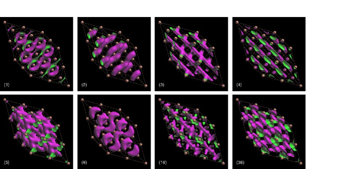
Figure 6: A subset of the optimal basis functions of fcc Cu, determined using 8 input k-points ($\Gamma$ plus seven images) and displayed in real-space in a $2\times 2\times 2$ supercell. Copper atom positions are indicated by copper-colored spheres. Ouside (inside) of basis function isosurfaces indicated in purple (green). Numbers in parentheses indicate the ordering in terms of overlap matrix eigenvalue magnitude corresponding to the following coverage of the entire space: (1) 7.6%; (2) 7.3%; (3) 6.4%; (4) 6.0%; (5) 5.7%; (6) 5.4%; (18) 1.8%; (36) 0.78%.

In the last decade, the use of maximally localized Wannier functions (MLWFs) has emerged as an extremely efficient and physically appealing route to interpolating electronic band structure and deriving useful tight-binding parameters from first-principles Hamiltonians (Marzari and Vanderbilt, 1997; Mostofi et al., 2008; Giustino et al., 2007a). The approach generates Wannier functions within a gauge which minimizes their spatial extent. In this sense, one constructs a set of basis functions localized in real-space, with one MLWF per band. The procedure is similar to that outlined in Figure 1, with the differences lying in an additional minimization of the spread of the orthogonalized basis functions and no requirement to construct a k-dependent Hamiltonian explicitly – this is obtained rather by Fourier interpolation. For systems with bands which do not possess an intrinsically local character ($sp$-bands in metals, for example) the Wannierization procedure has some intrinsic difficulties related to (i) providing a relatively large number of k-points to enable significant localization of the functions and (ii) disentangling such dispersive bands from manifolds of different character which they may easily cross due to their large dispersion. The latter problem was solved by Souza, Marzari, and Vanderbilt (Souza et al., 2002), while the former remains an intrinsic limitation imposed by the physical properties of the system under study. It is particularly problematic in spectroscopic studies where large numbers of unoccupied bands (which are in general dispersive) are needed.

In contrast with Wannier functions, the optimal basis functions used in Shirley interpolation have no constraint on their localization. They are simply the result of a diagonalization of the overlap matrix for the entire set of input periodic functions. In this sense, generating the optimal basis functions is quite automatic and does not suffer from issues common to most multidimensional minimization methods, such as trapping in local minima or sensitivity to initial conditions. The resulting functions can in fact be quite delocalized and, in general, we have not paid much attention to their spatial dependence, given that we do not try to exploit it in anyway. For instance, one could not hope to extract tight-binding parameters from a set of basis functions which are infinitely extended. Figure 6 shows a small number of the optimal basis functions derived for fcc Cu. They are clearly delocalized, and what look like simple functions for the larger eigenvalues of the overlap matrix become increasingly complex for smaller eigenvalues due to the requirements of orthonormality.

Shirley interpolation is particularly suited to exploration of metallic band structure, due to the robust automatic nature of generating the basis and the obviation of disentangling procedures. Furthermore, one can generate the band structure with very few initial k-points. In fact, we have already seen that for large supercells the $\Gamma$-point is sufficient to generate bands which accurately reproduce DFT calculations. Wannier interpolation requires more k-points to generate accurate band structure for bands which do not have an intrinsically localized character. For small (monatomic) primitive cells, this may not be problematic, but for larger supercells, where k-point sampling may still be necessary, then there are clear advantages to using Shirley interpolation.

Finally, it is worth mentioning that a combination of Shirley interpolation with the Wannierization procedure may be particularly effective for systems with intrinsic electron delocalization. Provided that one can generate a converged self-consistent charge density, one might use Shirley interpolation to efficiently generate solutions to the Kohn-Sham equations at as many k-points as desired and from these construct the necessary overlap matrix elements to begin the Wannierization procedure. This may prove particularly advantageous for the interpolation of metallic or high-energy unoccupied bands in large systems, such as metallic alloys, conducting polymers, etc.

VII Future Applications

The particular advantages of reducing the dimensions of a k-dependent Hamiltonian via an optimal basis are clear for explorations of band structure and spectroscopy. In this section, we outline further possibilities for improved algorithms or improved scaling in both DFT and beyond-DFT approaches.

Some self-consistent field calculations rely quite heavily on numerically converged Brillouin zone integrations. For example, an accurate determination of the Fermi-level is vital to an accurate estimation of the charge density in metallic systems, and charge transfer at metallic surfaces. For large system sizes, these calculations can prove prohibitively expensive, since the overall cost of the calculation scales like $N_{k}N^{3}$, where $N_{k}$ is the number of k-points and $N$ is the number of basis functions. Even though one can assume that larger simulation cells reduce the number of required k-points for numerical convergence, this may not be a sufficient to reduce the overall cost significantly. For example, doubling the system size would lead to scaling of $(N_{k}/2)(2N)^{3}=2^{2}(N_{k}N^{3})$, which is disheartening if $N_{k}/2>1$. Since we have seen now that for large systems one can quite easily generate accurate band energies and states throughout the Brillouin zone, one could in principle iteratively calculate just the zone-center electronic structure, while using interpolation to converge the Fermi-level and self-consistent charge density upon which the Kohn-Sham Hamiltonian is based. This would reduce the overall scaling, removing the linear dependence on $N_{k}$ at the expense of an increase in the overall prefactor associated with generating the optimal basis and k-dependent Hamiltonian.

For calculating excited state properties from first principles, the combination of the $GW$ approximation(HYBERTSEN and LOUIE, 1986) and Bethe-Salpeter Equation (BSE)(Rohlfing and Louie, 1998, 2000) has emerged as an accurate and efficient approach when applied to crystalline solids, molecules, nanostructures, and surfaces. This approach is computationally demanding (scaling at least as $N^{4}$) and relies heavily on access to detailed Brillouin zone sampling of the calculated electronic structure. For periodic systems, a very fine sampling of k-space is required to obtain converged BSE solutions, and interpolation procedures have already been applied to enable more efficient calculations. In fact, Shirley has already used this approach to deal with optical and x-ray excitations in solids (Benedict et al., 1998; Shirley, 1998). The main bottle-neck in such calculations comes from the need to access the dielectric matrix at many k-points. We hope to apply the Shirley interpolation scheme to improve the scaling of such calculations by representing the dielectric matrix within the Shirley basis. This will be the subject of future work.

VIII Conclusions

We have presented a new implementation of the Shirley interpolation method. The advances in our approach include: (1) a reduction in the number of input electronic structure calculations required to construct the optimal basis; (2) the ability to interpolate over the entire Brillouin zone using just the zone-center as input for systems with large unit cells; and (3) a generalization of the non-local potential which reduces storage requirements, permits the use of both norm-conserving and ultrasoft pseudopotentials. We provide applications of this method to sodium, $\gamma$-brass, graphene, and copper which illustrate its generality and robustness, particularly in treating metals. In this regard, it is competitive with existing interpolation schemes based on maximally-localized Wannier functions.