Coverage Optimization using Generalized Voronoi Partition

Abstract

In this paper a generalization of the Voronoi partition is used for optimal deployment of autonomous agents carrying sensors with heterogeneous capabilities, to maximize the sensor coverage. The generalized centroidal Voronoi configuration, in which the agents are located at the centroids of the corresponding generalized Voronoi cells, is shown to be a local optimal configuration. Simulation results are presented to illustrate the presented deployment strategy.

I Introduction

Technological advances in areas such as wireless communication, autonomous vehicular technology, computation, and sensors, facilitate the use of a large number of agents (UAVs, mobile robots, autonomous vehicles etc.) to cooperatively achieve various tasks in a distributed manner. One of the very useful applications of the multi-agent systems is in sensor networks, where a group of autonomous agents perform cooperative sensing of a large geographical area. Voronoi partition [1] has been used for optimal deployment of mobile agents carrying sensors [2, 3, 4]. This paper discusses a generalization of Voronoi partition to addresses heterogeneity of sensors in their capabilities.

The problem of optimal deployment of sensors has attracted many researchers [5]. Zou and Chakrabarty [6] use the concept of virtual force to solve this problem. Akbarzadeh et al. [7] use an evolutionary algorithm approach. Yao et al. [8] address a problem of camera placement for persistent surveillance. Murray et al. [9] address a problem of placing sensors such as video cameras for security monitoring. Kale and Salapaka [10] use heuristically designed algorithms based on maximum entropy to seek global minimum for a simultaneous resource location and multi-hop routing. The problem of optimal deployment of sensors belongs to a class of problems known as locational optimization or facility location [1, 11] in the literature, and when homogeneous sensors are used, a centroidal Voronoi configuration [12] is a standard solution for this class of problems. Cortes et al. [2, 13] use these concepts to formulate and solve the problem of optimal deployment of sensors. The authors provide rigorous mathematical results on spatial distribution, convergence, and other useful properties. Pimenta et al. [14] follow a similar approach to address a problem with heterogeneous robots, using power diagram (or Voronoi diagram in Laguerre geometry) to account for different footprints of the sensors. Kwok and Martínez [15] use power weighted and multiplicatively weighted Voronoi partitions to solve an energy aware limited range coverage problem. Pavone et al. [16] use power diagrams for equitable partitioning for robotic networks.

In the literature, sensors in a network are usually considered to be homogeneous in their capability. Whereas, in practical problems, the sensors may have different capabilities even though they are similar in their functionality. The heterogeneity in capabilities could be due to various reasons, the chief being the difference in specified performance. Though some researchers address optimal deployment of heterogeneous sensors (such as [14]), one of the well known generalization of the standard Voronoi partition (weighted Voronoi partition, Power diagram, etc.) is used to address heterogeneity. In this paper, we generalize the standard Voronoi partition to address a class of heterogeneous locational optimization problems, which include some of the problems addressed in the literature. We use node functions in place of the usual distance measure used in standard Voronoi partition and its variants. The mobile sensors are assumed to have heterogeneous capabilities in terms of their effectiveness. This paper presents a generalization of the optimal deployment concepts presented in [2, 13], using generalized Voronoi partition in place of the standard Voronoi partition. Some preliminary results have been reported in [17] earlier. This paper gives a more elaborate treatment.

II Generalization of the Voronoi partition

A generalization of the Voronoi partition, considering heterogeneity in the sensors’ capabilities, is presented here. Several extensions or generalizations of Voronoi partition to suit specific applications have been reported in the literature [1]. Herbert and Seidel [18] have introduced an approach in which, instead of the site set, a finite set of real-valued functions $f_{i}:D\mapsto\mathbb{R}$ were used to partition the domain $D$.

Let $I_{N}=\{1,2,\ldots,N\}$. Consider a space $Q\subset\mathbb{R}^{d}$ and a set of points called nodes or generators $\mathcal{P}=\{p_{1},p_{2},\ldots,p_{N}\}$, $p_{i}\in Q$, with $p_{i}\neq p_{j}$, whenever $i\neq j$. The Voronoi partition generated by $\mathcal{P}$ is the collection $\mathcal{V}(\mathcal{P})=\{V_{i}(\mathcal{P})\}_{i\in I_{N}}$, and is defined as,

$$V_{i}(\mathcal{P})=\left\{q\in Q|\parallel q-p_{i}\parallel\leq\parallel q-p_{j}\parallel,\forall p_{j}\in\mathcal{P},j\in I_{N}\right\}$$ (1)

where, $\parallel.\parallel$ denotes the Euclidean norm. The basic components of the Voronoi partition are: i) A space to be partitioned; ii) A set of sites, or nodes, or generators; and iii) A distance measure such as the Euclidean distance.

In this paper a generalization of the Voronoi partition is defined to suit the application, namely the heterogeneous locational optimization of sensors. This generalization has the following components: i) The domain of interest as the space to be partitioned; ii) The configuration of multi-agent system $\mathcal{P}$ as the site (or node or generator) set; and iii) A set of node functions in place of a distance measure. Consider strictly decreasing analytic functions $f_{i}:\mathbb{R}^{+}\mapsto\mathbb{R}$, where, $f_{i}$ is called a node function for the $i$-th node. Define generalized Voronoi partition of $Q$ with node configuration $\mathcal{P}$ and node functions $f_{i}$ as a collection $\mathcal{V}^{g}=\{V^{g}_{i}\}$, $i\in I_{N}$, with mutually disjoint interiors, such that $Q=\cup_{i\in I_{N}}V^{g}_{i}$, where $V^{g}_{i}$ is defined as

$$V^{g}_{i}=\{q\in Q|f_{i}(\|p_{i}-q\|)\geq f_{j}(\|p_{j}-q\|),\quad\forall j\neq i\text{,}j\in I_{N}\}$$ (2)

A generalized Voronoi cell $V^{g}_{i}$ can be topologically non-connected, null, and may contain other Voronoi cells. In the context of the problem discussed in this paper, $q\in V^{g}_{i}$ means that the $i$-th agent/sensor is the most effective in sensing at point $q$. This is reflected in the $\geq$ sign in the definition. In standard Voronoi partition used for the homogeneous case, $\leq$ sign for distances ensured that the $i$-th sensor is the most effective in $V_{i}$. (Note that $f_{i}$ are strictly decreasing.) The condition that $f_{i}$ are analytic implies that for every $i,j\in I_{N}$, $f_{i}-f_{j}$ is analytic. By the property of real analytic functions, the set of intersection points between any two node functions is a set of measure zero. This ensures that the intersection of any two cells is a set of measure zero, that is, the boundary of a cell is made up of the union of at most $d-1$ dimensional subsets of $\mathbb{R}^{d}$. Otherwise the requirement that the cells should have mutually disjoint interiors may be violated. Analyticity of the node functions $f_{i}$ is a sufficient condition to discount this possibility. Further, note that for some $i\neq j$, if $f_{i}\neq f_{j}$, then it is acceptable to have $p_{i}=p_{j}$. Only when $f_{i}=f_{j}$ and $i\neq j$, the condition $p_{i}\neq p_{j}$ is imposed in case of the generalized Voronoi partition (see Appendix for details). It can be shown that the centroid of a generalized Voronoi cell lies within its convex hull [19].

II-A Special cases 

A few interesting special cases of the generalized Voronoi partition are discussed below.

Case 1: Weighted Voronoi partition

Consider multiplicatively and additively weighted Voronoi partitions as special cases. Let $f_{i}(r_{i})=-\alpha_{i}r_{i}-d_{i}$ where, $r_{i}=\parallel p_{i}-q\parallel$ and, $\alpha_{i}$ and $d_{i}$ take finite positive real values for $i\in I_{N}$. Thus,

$$V^{w}_{i}=\{q\in Q|\alpha_{i}r_{i}+d_{i}\leq\alpha_{j}r_{j}+d_{j}\text{,}\quad\forall j\neq i\text{,}\quad j\in I_{N}\}$$ (3)

The partition $\mathcal{V}^{w}=\{V^{w}_{i}\}$ is called a multiplicatively and additively weighted Voronoi partition. $\alpha_{i}$ are called multiplicative weights and $d_{i}$ are called additive weights.

Case 2: Standard Voronoi partition

The standard Voronoi partition can be obtained as a special case of (2) when the node functions are $f_{i}(r_{i})=-r_{i}$. It can be shown that if the node functions are homogeneous ($f_{i}(\cdot)=f(\cdot)$ for each $i\in I_{N}$), then the generalized Voronoi partition gives the standard Voronoi partition.

Case 3: Power diagram

Power diagram or Voronoi diagram in Laguerre geometry $\mathcal{V}^{LG}=\{V^{LG}_{i}\}$ is defined as $V^{LG}_{i}=\{q\in Q|d_{p}(q,p_{i})\leq d_{p}(q,p_{j})\text{,}i\neq j\},i,j\in I_{N}$ where, $d_{p}(q,p_{i})=\|p_{i}-q\|^{2}-R^{2}_{p_{i}}$, the power distance between $q$ and $p_{i}$, with $R_{p_{i}}>0$ being a parameter fixed for a given node $p_{i}$. In the context of robot coverage problem addressed in [14], $R_{P_{i}}$ represents the radius of the footprint of the $i$-th robot. It is easy to see that the power diagram can be obtained from the generalized Voronoi partition (2) by setting $f_{i}(\|q-p_{i}\|)=-(\|p_{i}-q\|^{2}-R^{2}_{p_{i}})$ with $R_{P_{i}}$ as a parameter specific to each node function.

Case 5: Other possible variations

Other possible variations of the Voronoi partition are using objects such as lines, curves, discs, polytopes, etc. other than points as sites/nodes, generalization of the space to be partitioned, and use of non-Euclidean metrics or pseudo-metrics. It is easy to verify that these generalizations can also be obtained by suitable selection of site sets, spaces, and node functions.

III Heterogeneous locational optimization problem

The heterogeneous locational optimization problem (HLOP) for a mobile sensor network is formulated and solved here. Let $Q\subset\mathbb{R}^{d}$ be a convex polytope, the space in which the sensors have to be deployed; $\phi:Q\mapsto[0,1]$, be a density distribution function, with $\phi(q)$ indicating the probability of an event of interest occurring at $q\in Q$, indicating the importance of measurement at $q$; $\mathcal{P}(t)=\{p_{1}(t),p_{2}(t),\ldots,p_{N}(t)\},i\in I_{N}$, $p_{i}(t)\in Q$ be the configuration of $N$ sensors at time $t$, with $p_{i}(0)\neq p_{j}(0),\forall i\neq j$; $f_{i}:\mathbb{R}^{+}\mapsto\mathbb{R}$, $i\in I_{N}$, be analytic, strictly decreasing function corresponding to the $i$-th node, the sensor effectiveness function of $i$-th agent, with $f_{i}(\|p_{i}-q\|)$ indicating the effectiveness of the $i$-th sensor located at $p_{i}\in Q$, in sensing at a point $q\in Q$. It is natural to assume $f_{i}$ to be strictly decreasing. The objective of the problem is to deploy the mobile sensors in $Q$ so as to maximize the probability of detection of an event of interest.

In case of homogeneous sensors [2], the sensor located in Voronoi cell $V_{i}$ is closest to all the points $q\in V_{i}$ and hence, by the strictly decreasing variation of sensor’s effectiveness with distance, most effective within $V_{i}$. Thus, the Voronoi decomposition leads to optimal partitioning of the space in the sense that each sensor is most effective within its Voronoi cell. In the heterogeneous case too, it is easy to see that each sensor is most effective within its generalized Voronoi cell. Now, as the partitioning is optimal, the problem is to find the location of each sensor within its generalized Voronoi cell.

The objective function

Consider the following objective function to be maximized,

$$\mathcal{H}(\mathcal{P})=\int_{Q}\max_{i\in I_{N}}\{f_{i}(\|q-p_{i}\|)\}\phi(q)dQ=\sum_{i\in I_{N}}\int_{V^{g}_{i}}f_{i}(\|q-p_{i}\|)\phi(q)dQ$$ (4)

Note that the generalized Voronoi decomposition splits the objective function into a sum of contributions from each generalized Voronoi cell. Hence the optimization problem can be solved in a spatially distributed manner, that is, the optimal configuration can be achieved by each sensor solving only that part of the objective function which corresponds to its own cell, using only local information. Note also that the objective function has the same form as in [2] where a similar problem is addressed for homogeneous sensors.

By generalizing results in [19] (Proposition 2.23 in [19]), it can be shown that the gradient of the objective function (4) with respect to $p_{i}$ is

$$\frac{\partial\mathcal{H}}{\partial p_{i}}=\int_{V^{g}_{i}}\phi(q)\frac{\partial f_{i}(r_{i})}{\partial p_{i}}dQ$$ (5)

The critical points

By suitably generalizing the concepts in [19], it can be shown that the gradient of the objective function (4) with respect to $p_{i}$ is

$$\frac{\partial\mathcal{H}}{\partial p_{i}}=\int_{V^{g}_{i}}\phi(q)\frac{\partial f_{i}(r_{i})}{\partial p_{i}}dQ=-\int_{V^{g}_{i}}\tilde{\phi^{i}}(q,p_{i})(p_{i}-q)dQ=-\tilde{M}_{V^{g}_{i}}(p_{i}-\tilde{C}_{V^{g}_{i}})$$ (6)

where, $\tilde{\phi^{i}}(q,p_{i})=-2\phi(q)\frac{\partial f_{i}(r_{i})}{\partial{(r_{i}}^{2})}$. As $f_{i}$s are strictly decreasing, $\tilde{\phi}(q)$ is always non-negative. Hence, $\tilde{\phi}$ can be interpreted as density modified or perceived by the sensors, $\tilde{M}_{V^{g}_{i}}$ as mass, and $\tilde{C}_{V^{g}_{i}}$ as centroid of the cell $V^{g}_{i}$. Thus, the critical points/configurations are $\mathcal{P}^{*}=\{\mathcal{P}|p_{i}=\tilde{C}_{V^{g}_{i}}(\mathcal{P}),i\in I_{N}\}$, and such a configuration $\mathcal{P}^{*}$, of agents is called a generalized centroidal Voronoi configuration.

The critical points are not unique, as with the standard Voronoi partition. But in the case of the generalized Voronoi partition, some of the cells could become null. Further, as in the case of homogenous sensors (that is, using standard Voronoi partition), the critical points/configuration correspond to local minima of the objective function (4).

III-A The control law

Consider the agent dynamics and control law as

$$\dot{p}_{i}(t) = u_{i}(t)$$ (7)

$$u_{i}(t) = -k_{prop}(p_{i}(t)-\tilde{C}_{V_{i}}(t))$$ (8)

Control law (8) makes the mobile sensors move toward $\tilde{C}_{V^{g}_{i}}$ for positive $k_{prop}$. If, for some $i\in I_{N}$, $V^{g}_{i}=\emptyset$, then set $\tilde{C}_{V^{g}_{i}}=p_{i}$. We restrict the analysis to the simple first order dynamics under the assumption, that there is a low-level controller which can cancel the actual dynamics of the agents and enforce (7).

Theorem 1

The trajectories of the sensors governed by the control law (8), starting from any initial condition $\mathcal{P}(0)$, will asymptotically converge to the critical points of $\mathcal{H}$.

Proof.  Consider $V(\mathcal{P})=-\mathcal{H}$.

$${\dot{V}}(\mathcal{P})=-\frac{d\mathcal{H}}{dt}=-\sum_{i\in I_{N}}\frac{\partial\mathcal{H}}{\partial p_{i}}\dot{p}_{i}=-k_{prop}\sum_{i\in I_{N}}\tilde{M}_{V^{g}_{i}}(p_{i}-\tilde{C}_{V^{g}_{i}})^{2}$$ (9)

Let $p_{i}\in\partial Q$, the boundary of $Q$ for some $i$ at some time $t$. The vector $\dot{p}_{i}=-k_{prop}(p_{i}-\tilde{C}_{V^{g}_{i}})$ always points inward to $Q$ or is tangential to $\partial Q$ at $p_{i}$ as $\tilde{C}_{V^{g}_{i}}\in Q$ (Note that $\text{co}(V^{g}_{i})\subset Q$). Thus, by Theorem 3.1 in [20], the set $Q$ is invariant under the closed-loop dynamics given by (7) and (8).

Further, observe that, $V:Q^{N}\mapsto\mathbb{R}$ is continuously differentiable in $Q$ as $\{V^{g}_{i}\}$ depends continuously on $\mathcal{P}$ by Theorem A3; $Q^{N}$ is a compact invariant set; ${\dot{V}}$ is negative semi-definite in $Q^{N}$; $E=\dot{V}^{-1}(0)=\{\tilde{C}_{V^{g}_{i}}\}$, which itself is the largest invariant subset of $E$ by the control law (8). Thus, by LaSalle’s invariance principle, the trajectories of the agents governed by control law (8), starting from any initial configuration $\mathcal{P}(0)$ (Note that $p_{i}(0)\in Q,\forall i\in I_{N}$), will asymptotically converge to set $E$, the critical points of $\mathcal{H}$, that is, the centroids of the generalized centroidal Voronoi cells with respect to the density function as perceived by the sensors. $\Box$

Note that a similar result is provided in [2, 19] for homogeneous sensors using standard Voronoi partition. Further, We had assumed $p_{i}(0)\neq p_{j}(0),\forall i\neq j$. If $f_{i}\neq f_{j},\forall i\neq j$, then it is possible that $p_{i}(t)=p_{j}(t)$ at some time $t>0$. However, if for any $i\neq j$, $f_{i}(\cdot)=f_{j}(\cdot)$, then $p_{i}(t)\neq p_{j}(t),\forall t>0$. Thus, the state space is not the entire $Q^{N}$, and hence not necessarily compact. An extension to LaSalle’s invariance principle in such a situation is provided in [19], which can be used here for proving the convergence result, in such a scenario.

It should be noted that the gradient based control law (8) can only guarantee local maximum of the objective function (4). Techniques such as deterministic annealing can be used to solve the global optimization problem [21, 22, 23].

IV Limited range sensors

In the previous sections, it was assumed that the sensors have infinite range but with diminishing effectiveness. However, in reality the sensors will have limited range. In this section a spatially distributed limited range locational optimization problem is formulated. In [13] authors address the effect of limit on the sensor range using standard Voronoi partition. The results provided here are based on and extension of those results.

Let $R_{i}$ be the limit on range of the sensors and $\bar{B}(p_{i},R_{i})$ be a closed ball centered at $p_{i}$ with a radius of $R_{i}$. The $i$-th sensor has access to information only from points in the set $V^{g}_{i}\cap\bar{B}(p_{i},R_{i})$. Consider $\hat{f}_{i}$ which is continuously differentiable in $[0,R_{i}]$, with $\hat{f}_{i}(R_{i})=0$, and $\hat{f}_{i}(r)=0,\forall r>R_{i}$ as the sensor effectiveness function. This function models the effectiveness of a sensor having a limit of $R_{i}$ on its range. Note that the derivative of $\hat{f}_{i}$ can have a discontinuity at $r=R_{i}^{+}$, where $R_{i}^{+}=\lim_{h\rightarrow 0}(R_{i}+h)$. Consider the following objective function to be maximized,

$$\hat{\mathcal{H}}(\mathcal{P})=\sum_{i\in I_{N}}\int_{(V^{g}_{i}\cap\bar{B}(p_{i},R_{i}))}\phi(q)\hat{f_{i}}(\|p_{i}-q\|))dQ$$ (10)

It can be noted that the objective function is made up of sums of the contributions from sets $V^{g}_{i}\cap\bar{B}(p_{i},R_{i})$, enabling the sensors to solve the optimization problem in a spatially distributed manner. By generalizing the results in [13], it can be shown that the gradient of the multi-center objective function (10) with respect to $p_{i}$ is given by

$$\frac{\partial\hat{\mathcal{H}}}{\partial p_{i}}=\int_{(V^{g}_{i}\cap\bar{B}(p_{i},R_{i}))}\phi(q)\frac{\partial}{\partial p_{i}}\hat{f_{i}}(\|p_{i}-q\|)dQ$$ (11)

Thus, the gradient of the objective function (10) is

$$\frac{\partial\hat{\mathcal{H}}(\mathcal{P})}{\partial p_{i}}=-\tilde{M}_{(V^{g}_{i}\cap\bar{B}(p_{i},R_{i}))}(p_{i}-\tilde{C}_{(V^{g}_{i}\cap\bar{B}(p_{i},R_{i}))})$$ (12)

where, the mass $\tilde{M}_{(V^{g}_{i}\cap\bar{B}(p_{i},R_{i}))}$ and the centroid $\tilde{C}_{(V^{g}_{i}\cap\bar{B}(p_{i},R_{i}))}$ are now computed within the region $(V^{g}_{i}\cap\bar{B}(p_{i},R_{i}))$, that is, the region of Voronoi cell $V^{g}_{i}$, which is accessible to the $i$-th robot. The critical points/configurations are $\mathcal{P}^{*}=\{\mathcal{P}|p_{i}=\tilde{C}_{(V^{g}_{i}\cap\bar{B}(p_{i},R_{i}))}(\mathcal{P}),i\in I_{N}\}$.

Consider the following control law to guide the agents toward the respective centroids

$$u_{i}=-k_{prop}(p_{i}-\tilde{C}_{(V^{g}_{i}\cap\bar{B}(p_{i},R_{i}))})$$ (13)

Further, by generalizing the corresponding results in [13], it can be shown that the trajectories of the sensors governed by the control law (13), starting from any initial condition $\mathcal{P}(0)$, will asymptotically converge to the critical points of $\hat{\mathcal{H}}$.

V Simulation Experiments

In this section we provide results of a set of simulation experiments to validate the performance of the proposed deployment strategy. The space is discretized into hexagonal cells, which are preferred over square or rectangular cells because of the fact that in hexagonal grids all the neighboring cells are at equal distance. We have considered $f_{i}(r_{i})=k_{i}e^{-\alpha_{i}{r_{i}}^{2}}$ as node functions. Three density distributions have been used: i) a uniform density, ii) an exponential density distribution $\phi(x,y)=0.9e^{-0.001((x-42)^{2}+(y-36)^{2})}$ having a peak near the center of space, and iii) an exponential density distribution $\phi(x,y)=0.9e^{-0.001((x-70)^{2}+(y-60)^{2})}$ having peak toward the corner of the space. The space considered is a rectangular area with x-axis range of 0 to 86 units and y-axis range of 0 to 74 units. The (locally) optimal deployment is achieved when each of the agents are located at the respective centroids. Each hexagonal cell measures 1 unit from center to any of its corners. A normalized error measure of how close the agents are to the centroid at the $n$-th time step is defined as $error(n)=(\sum_{m=1}^{N}\|(p_{m}(n)-\tilde{C}_{V^{g}_{m}}(n))\|^{2})/\max_{i\in I_{M}}(error(i))$, where $M$ is the total number of time steps to achieve the optimal deployment. Simulations were carried out by either fixing $k_{i}$ or $\alpha_{i}$, or varying both. The case of both $k_{i}$ and $\alpha_{i}$ fixed corresponds to the homogeneous agent case and leads to a standard Voronoi partition.

Figures 2, 4, and 6 show the trajectories of agents with exponential density having peak near the center, exponential density having peak near the corner, and an uniform density. Figures 2(a), 4(a), and 6(a) correspond to cases where all the agents have the same $\alpha_{i}$, but different $k_{i}$. Figures 2(b), 4(b), and 6(b) correspond to case where all the agents have the same $k_{i}$ and different $\alpha_{i}$. Figures 2(c), 4(c), and 6(c) correspond to cases where all the agents have different $k_{i}$ and $\alpha_{i}$. When $k_{i}$ is fixed, it leads to multiplicatively weighted Voronoi partition, when $\alpha_{i}$ is fixed it leads to a generalized Voronoi partition with intersection between any two cells being a straight line segment, and when both $k_{i}$ and $\alpha_{i}$ vary, it leads to a generalized Voronoi partition. A contour plot is also shown for exponential density cases. It can be observed that the agents move toward the peak of density. Dots indicate the starting position of agents and ‘o’s indicate the final position. Figures 2, 4, and 6 show the history of error and the objective functions for the corresponding simulations. In all cases the error reduces and the objective function is (locally) maximized.

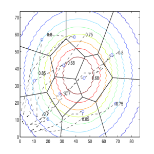
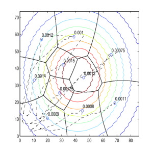
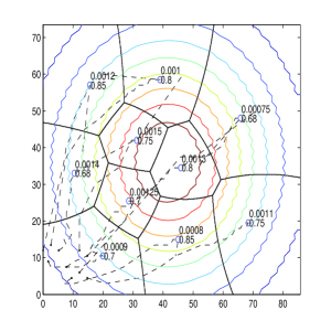
Figure 1: Trajectories of agents with exponential density having peak at the center of space, and a) $\alpha$ fixed and $k$ varying b) $\alpha$ varying and $k$ fixed c) both $\alpha$ and $k$ varying.

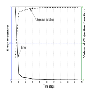
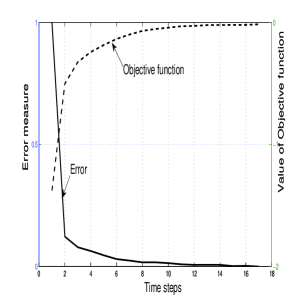
Figure 2: History of error and value of objective function with exponential density having peak at the center of space, and a) $\alpha$ fixed and $k$ varying b) $\alpha$ varying and $k$ fixed c) both $\alpha$ and $k$ varying.

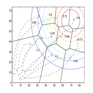
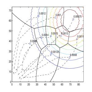
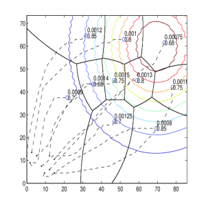
Figure 3: Trajectories of agents with exponential density having peak toward the corner of space, and a) $\alpha$ fixed and $k$ varying b) $\alpha$ varying and $k$ fixed c) both $\alpha$ and $k$ varying.

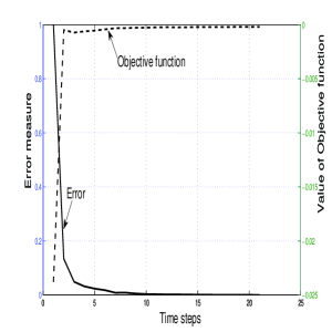
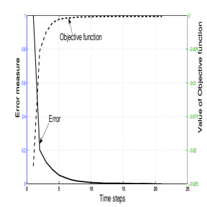
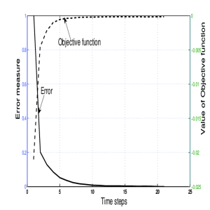
Figure 4: History of error and value of objective function with exponential density having peak toward the corner of space, and a) $\alpha$ fixed and $k$ varying b) $\alpha$ varying and $k$ fixed c) both $\alpha$ and $k$ varying.

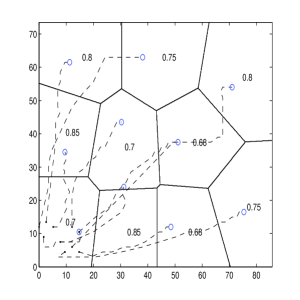
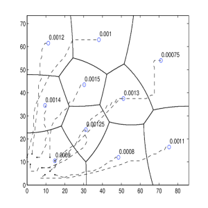
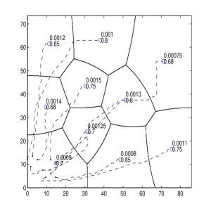
Figure 5: Trajectories of agents with uniform density, and a) $\alpha$ fixed and $k$ varying b) $\alpha$ varying and $k$ fixed c) both $\alpha$ and $k$ varying.

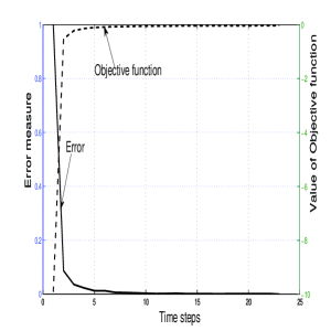
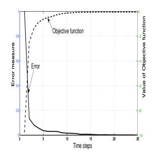
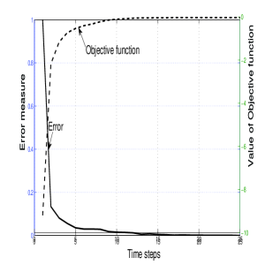
Figure 6: History of error and value of objective function with uniform density, and a) $\alpha$ fixed and $k$ varying b) $\alpha$ varying and $k$ fixed c) both $\alpha$ and $k$ varying.

VI Conclusions

A generalization of Voronoi partition has been proposed and the standard Voronoi decomposition and its variations are shown to be special cases of this generailzation. The problem of optimal deployment of agents carrying sensors with heterogeneous capabilities has been formulated and solved using the generalized Voronoi partition. The generalized centroidal Voronoi configuration was shown to be a locally optimal configuration. Illustrative simulation results were provided to support the theoretical results.

The generalization of Voronoi partition and the heterogeneous locational optimization techniques can be applied to a wide variety of problems, such as spraying insecticides, painting by multiple robots with heterogeneous sprayers, and many others. The heterogeneous locational optimization problems can find applications outside robotics field. One such problem is of deciding on optimal location for public facilities.The generalization of Voronoi partition presented also provides new challenges for developing efficient algorithms for computations related to the generalized Voronoi partition, and characterizing its properties.

Appendix: On continuity of generalized Voronoi partition

A proof on the continuity of the generalized Voronoi partition is provided here. The treatment provided here is kept informal, but discusses major steps for a more elaborate mathematical proof, which is beyond the scope of this paper.

Consider a partition $\mathcal{W}(\mathcal{P})=\{W_{i}(\mathcal{P})\}\text{,}i\in I_{N}$ of $Q\subset\mathbb{R}^{2}$ with $\mathcal{P}=\{p_{1},p_{2},\ldots,p_{N}\}$, $p_{i}\in Q$. Let $\partial{W}_{i}(\mathcal{P})$ be the bounding (closed) curve of cell $W_{i}$, parameterized by a parameter $u_{i}(\mathcal{P})\in[0,1]$. The partition $\mathcal{W}(\mathcal{P})$ is said to be continuous in $\mathcal{P}$ if and only if each of the $u_{i}(\mathcal{P})$ is continuous in $\mathcal{P}$. That is, the cell boundaries move smoothly with configuration of sites $\mathcal{P}$. This is an important property needed for proving the stability and convergence of the agent motion under the influence of the proposed control law using LaSalle’s invariance principle. This understanding of continuity of a partition can be extended to a general $d$-dimensional Euclidean space. Now, in $\mathbb{R}^{d}$, $\partial W_{i}$ are hypersurfaces in $d$-dimensional Euclidean space and $u_{i}$ are vector valued functions of dimension $d-1$. Continuity of $u^{j}_{i}$, the $j$-th component of $u_{i}$ with $\mathcal{P}$ for each $i\in I_{N}$ and $j\in I_{d-1}$ ensures the continuity of $\mathcal{W}(\mathcal{P})$ when $Q\subset\mathbb{R}^{d}$.

Now consider the continuity of standard Voronoi partition. It is well known that as long as $p_{i}\neq p_{j}$, whenever $i\neq j$, $\mathcal{V}(\mathcal{P})$, the standard Voronoi partition, is continuous in $\mathcal{P}$. This continuity is due to continuity of the Euclidean distance. It is interesting to see what happens when $p_{i}=p_{j}$ for some $i\neq j$. Consider $i\neq j$ and let $p_{i}(0)\neq p_{j}(0)$. Now, $V_{i}$ and $V_{j}$ are distinct sets such that $V_{i}\cap V_{j}$ is either null or is the common boundary between them, which is a straight line segment of the perpendicular bisector of the line joining $p_{i}$ and $p_{j}$. Let $V_{i}\cap V_{j}\neq\emptyset$, that is, the agents $i$ and $j$ are Voronoi neighbors, and agent $i$ is stationary while agent $j$ is moving toward $i$. This causes $V_{i}$ to shrink and $V_{j}$ to expand as the common boundary between them moves closer to $p_{i}$. But, when $p_{j}(t)=p_{i}(t)$, $V_{i}(t)=V_{j}(t)=V_{i}(0)\cup V_{j}(0)$, which is a sudden jump, and boundaries of both $V_{i}$ and $V_{j}$ jump, leading to discontinuity. Thus, $\mathcal{V}(\mathcal{P})$ is discontinuous whenever there is a transition between $p_{i}\neq p_{j}$ and $p_{i}=p_{j}$, for some $i\neq j$. Similar discontinuity, as in the standard Voronoi partition with $\mathcal{P}$, can occur in the case of generalized Voronoi partition, whenever $p_{i}$ and $p_{j}$ are Voronoi neighbors and $f_{i}=f_{j}$. This is illustrated in Figure 7. The line segment separating $V^{g}_{1}$ and $V^{g}_{2}$ disappears when $p_{1}=p_{2}$ and the corresponding Voronoi cells jump in their size. In fact $V^{g}_{1}$ and $V^{g}_{2}$ jump to $V^{g}_{1}\cap V^{g}_{2}$, and the common boundary between $V^{g}_{1}$ and $V^{g}_{2}$ jumps to the boundary of $V^{g}_{1}\cap V^{g}_{2}$.

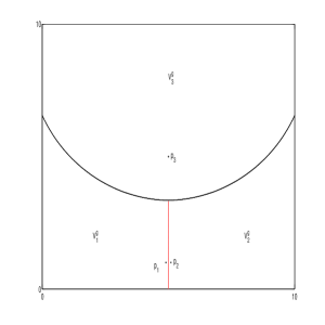
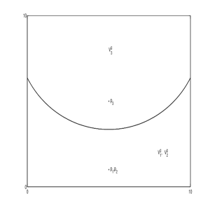
Figure 7: Illustration of discontinuity of Voronoi partition at $p_{1}=p_{2}$ when $f_{1}=f_{2}$. The straight line segment separating $V^{g}_{1}$ and $V^{g}_{2}$ suddenly disappears when two points $p_{1}$ and $p_{2}$ merge.

In case of the standard Voronoi partition, if $p_{i}(0)\neq p_{j}(0)$, whenever $i\neq j$, the control law ensures that $p_{i}(t)\neq p_{j}(t)$, whenever $i\neq j$, $\forall t>0$. If two agents are together to start with, that is, $p_{i}(0)=p_{j}(0)$, whenever $i\neq j$, then the control law ensures that they are always together. This is due to the fact that $\tilde{C}_{V_{i}}\in V_{i}$, $\forall i\in I_{N}$. This is not always true in case of the generalized Voronoi partition. Thus, the issue of continuity of generalized Voronoi partition is a more involved one.

Condition A. There is no transition from $\mathcal{P}(t)$ to $\mathcal{P}(t^{\prime})$, such that $p_{i}(t)\neq p_{j}(t)$ and $p_{i}(t^{\prime})=p_{j}(t^{\prime})$, for all pairs $(i,j)$, $i\neq j$, $i,j\in I_{N}$, and $f_{i}=f_{j}$.

As discussed earlier, violation of the condition A can cause discontinuity in the generalized Voronoi partition.

Lemma A1: The generalized Voronoi partition depends continuously on $\mathcal{P}$ if condition A is satisfied.

Outline of the proof:  Let us consider any two agents $i$ and $j$ which are Voronoi neighbors, take up three distinct and exhaustive cases, and prove the continuity for each of them.

Case i) No two node functions are identical, that is, $(f_{i}-f_{j})\neq 0$, whenever $i\neq j$, and $V^{g}_{i}\neq\emptyset$, $\forall i\in I_{N}$. $\forall\mathcal{P}$.

All the points $q\in Q$ on the boundary common to $V^{g}_{i}$ and $V^{g}_{j}$ is given by $\{q\in Q|f_{i}(\|p_{i}-q\|)=f_{j}(\|p_{j}-q\|)\}$, that is, the intersection of the corresponding node functions. Let the $j$-th agent move by a small distance $dp$. This makes a point $q\in Q$, on the common boundary between $V_{i}$ and $V_{j}$ move by a distance, say $dx$. Now, as the node functions are strictly decreasing and are continuous, it is easy to see that $dx\rightarrow 0$ as $dp\rightarrow 0$. This is true for any two $i$ and $j$, and any $q$ on the common boundary between $V^{g}_{i}$ and $V^{g}_{j}$. Thus, the generalized Voronoi partition depends continuously on $\mathcal{P}$. Note that it is easy to verify that $p_{i}=p_{j}$ for $i\neq j$ does not lead to discontinuity in this case.

Case ii) No two node functions are identical, that is, $(f_{i}-f_{j})\neq 0$, whenever $i\neq j$, and $\mathcal{P}$ is such that $V^{g}_{i}=\emptyset$ for some $i\in I_{N}$.

Let both $V^{g}_{i}$ and $V^{g}_{j}$ be non null sets, and $V^{g}_{i}\subset V^{g}_{j}$ for some $\mathcal{P}$. Now with evolution of $\mathcal{P}$ in time, let $V^{g}_{i}=\emptyset$ for some $\mathcal{P^{\prime}}=\mathcal{P}+\delta\mathcal{P}$. The quantity $\int_{V^{g}_{i}}dQ$, and the common boundary vanish gradually to zero as the agent configuration changes from $\mathcal{P}$ to $\mathcal{P^{\prime}}$. Further, there is no jump in the boundary or size of the (generalized) Voronoi cell, or in the common boundary as in the case of standard Voronoi cell when there is a transition from $p_{i}\neq p_{j}$ to $p_{i}=p_{j}$.

Case iii). For some $i\neq j$, $f_{i}=f_{j}$. In this case, the common boundary between $V^{g}_{i}$ and $V^{g}_{j}$ is a segment of the perpendicular bisector of line joining $p_{i}$ and $p_{j}$. As in the case of standard Voronoi diagram, if agents $i$ and $j$ are neighbors and there is a transition from $p_{i}\neq p_{j}$ to $p_{i}=p_{j}$, the $\mathcal{V}^{g}(\mathcal{P})$ will have discontinuity. However, if condition A is satisfied, such a discontinuity will not occur.

Thus, as long as the condition A is satisfied, the generalized Voronoi partition depends continuously on $\mathcal{P}$. $\Box$

Lemma A2:  The control law (8) ensures that condition A is satisfied for all $\mathcal{P}$ if $p_{i}(0)\neq p_{j}(0)$ for all pairs $(i,j),i,j\in I_{N},i\neq j$, for which $f_{i}=f_{j}$.

Proof. Condition A can be violated only for pair $(i,j)$ for which $f_{i}=f_{j}$. As $p_{i}(0)\neq p_{j}(0)$, condition A will be violated if at some time $t$, $p_{i}(t)=p_{j}(t)$. Now $\tilde{C}_{V^{g}_{i}}$ will lie within the half plane $\{q\in Q|\|q-p_{i}\|<\|q-p_{j}\|\}$ and hence the control law cannot make the agent $i$ cross the common boundary between $i$ and $j$. Similarly, agent $j$ too cannot cross the boundary. Hence, if $p_{i}(0)\neq p_{j}(0)$, then $p_{i}(t)\neq p_{j}(t)$ for any $t\in\mathbb{R}$. Thus, the condition A cannot be violated. $\Box$

Theorem A3:  If $\mathcal{P}(0)$ is such that $p_{i}(0)\neq p_{j}(0)$ for all pairs $(i,j),i,j\in I_{N},i\neq j$, for which $f_{i}=f_{j}$, and the agents move according to the control law (8), then the generalized Voronoi partition depends continuously on $\mathcal{P}$.

Proof.  The proof follows from Lemmas A1 and A2. $\Box$

References

- [1] A. Okabe and A. Suzuki, Locational optimization problems solved through Voronoi diagrams, Eurpean Journal of Operations Research, vol. 98, no. 3, 1997, pp. 445-456.
- [2] J. Cortes, S. Martinez, T. Karata, and F. Bullo, Coverage control for mobile sensing networks, IEEE Transactions on Robotics and Automation, vol. 20, no. 2, 2004, pp. 243-255.
- [3] Guruprasad K.R. and D. Ghose, Automated multi-agent search using centroidal voronoi configuration, IEEE Tansactions on Automation Science and Engineering, vol. 8, issue 2, April 2011, pp. 420 - 423.
- [4] Guruprasad K.R. and D. Ghose, Performance of a class of multi-robot deploy and search strategies based on centroidal Voronoi configurations, International Journal of Systems Science, to appear.
- [5] C. G. Cassandras and W. Li, Sensor networks and cooperative control, European J. Control, vol. 11, no. 4-5, 2005, pp. 436-463.
- [6] Y. Zou and K. Chakrabarty, Sensor deployment and target localization baesd on virtual forces, Proc. of IEEE INFOCOM, 2003, pp. 1293-1303.
- [7] V. Akbarzadeh, A. Hung-Ren Ko, C. Gagn and M. Parizeau, Topography-aware sensor deployment optimization with CMA-ES, Parallel Problem Solving From Nature - PPSN XI, Lecture Notes in Computer Science, vol. 6239, 2011, pp. 141-150.
- [8] Y. Yao, C-H. Chen, B. Abidi, D. Page, A. Koschan, and M. Abidi, Can you see me now? sensor positioning for automated and persistent surveillance, IEEE Transactions on Systems, Man, and Cybernetics, Part B: Cybernetics, vol. 40, issue 1, 2010, pp. 101 - 115.
- [9] A.T. Murray, K. Kim, J.W. Davis, R. Machiraju, and R. Parent, Coverage optimization to support security monitoring, Computers, Environment and Urban Systems, vol. 31, 2007, pp. 133-147.
- [10] N. Kale and S. Salapaka, Maximum entropy principle based algorithm for simultaneous resource location and multi-hop routing in multi-agent networks, IEEE Transactions on Mobile Computing, to appear.
- [11] Z. Drezner, Facility Location: A Survey of Applications and Methods, New York, NY: Springer, 1995.
- [12] Q. Du, V. Faber and M. Gunzburger, Centroidal Voronoi tessellations: applications and algorithms, SIAM Review, vol. 41, no. 4, 1999, pp. 637-676.
- [13] J. Cortes, S. Martinez, and F. Bullo, Spatially-distributed coverage optimization and control with limited-range interactions, ESAIM: Control, Optimization and Calculus of Variations, vol. 11, no. 4, 2005, pp. 691-719.
- [14] L.C.A. Pimenta, V. Kumar, R.C. Mesquita, and A.S. Pereira, Sensing and coverage for a network of heterogeneous robots, Proceedings of IEEE Conference on Decision and Control, Cancun, December 2008, pp 3947 - 3952 .
- [15] A. Kwok and S. Martínez, Deployment algorithms for a power-constrained mobile sensor network, International Journal of Robust and Nonlinear Control, vol. 20, issue 7, 2002, pp. 745-763.
- [16] M. Pavone, A. Arsie, E. Frazzoli, and F. Bullo, Equitable partitioning policies for robotic networks, Proc of the 2009 IEEE International Conference on Robotics and Automation, Kobe, Japan, 2009, pp. 3979-3984.
- [17] K.R. Guruprasad and D. Ghose, Heterogeneous sensor based Voronoi decomposition for spatially distributed limited range locational optimization, in Voronoi’s Impact on Modern Science, Book 4, vol. 2, Proceedings of 5th Annual International Symposium on Voronoi Diagrams (ISVD 2008), Kiev, Ukraine, September 2008, pp. 78-87.
- [18] H. Edelsbrunner and R. Seidel, Voronoi diagrams and arrangements, Discrete Comput. Geom., vol 1, 1986, pp. 25-44.
- [19] F. Bullo, J. Cortes, S. Martinez, Distributed Control of Robotic Networks, Applied Mathematics Series, Princeton NJ, Princeton University press, 2009.
- [20] F. Blanchini, Set invariance in control, Automatica, vol. 35, 1999, pp. 1747-1767.
- [21] S. Salapaka, A. Khalak, and M.A. Dahleh, Constraints on locational optimization problems, Proc of the 42nd IEEE Conference on Decision and Control, Maui, Hawaii, USA, December, 2003, pp. 1741-1746.
- [22] K. Rose, Deterministic annealing for clustering, compression, classification, regression and related optimization problems, Procedings of IEEE, vol. 86, no. 11, 1998, pp. 2210-2239.
- [23] P. Sharma, S. Salapaka, and C. Beck, A Scalable Approach to Combinatorial Library Design for Drug Discovery, J. Chem. Inf. Model., vol. 48, no. 1, 2008, 48 (1), pp 27 41 pp. 27 41.