Anisotropic microwave conductivity of cuprate superconductors in the presence of CuO chain induced impurities

Abstract

The anisotropy in the microwave conductivity of the ortho-II YBa₂Cu₃O_6.50 is studied within the kinetic energy driven superconducting mechanism. The ortho-II YBa₂Cu₃O_6.50 is characterized by a periodic alternative of filled and empty $\hat{b}$-axis CuO chains. By considering the CuO chain induced extended anisotropy impurity scattering, the main features of the anisotropy in the microwave conductivity of the ortho-II YBa₂Cu₃O_6.50 are reproduced based on the nodal approximation of the quasiparticle excitations and scattering processes, including the intensity and lineshape of the energy and temperature dependence of the $\hat{a}$-axis and $\hat{b}$-axis microwave conductivities. Our results also confirm that the $\hat{b}$-axis CuO chain induced impurity is the main source of the anisotropy.

I Introduction

Impurity plays a crucial role in determining the behavior of many measurable properties of cuprate superconductors hirschfeld1 , such as the quasiparticle transport in the superconducting (SC) state. This follows from a fact that the physical properties of cuprate superconductors in the SC state are extreme sensitivity to the impurity effect than the conventional superconductors due to the finite angular-momentum charge carrier Cooper pairing with the d-wave symmetry hirschfeld1 . The single common feature is the presence of the CuO₂ plane shen , and it seems evident that the unusual behaviors of cuprate superconductors are dominated by this CuO₂ plane anderson . Experimentally, over twenty years measurements of electrodynamic properties at microwave energies have provided rather detailed information on the quasiparticle transport of cuprate superconductors bonn ; sflee ; hosseini ; turner ; harris ; bobowski , where the nodal quasiparticle spectrum contains most of the features expected for weak-limit impurity scattering. The early microwave conductivity measurements bonn ; sflee ; hosseini ; turner showed the microwave conductivity spectrum is CuO₂ plane isotropic. However, the recent development of a sufficient number of fixed-energy cavity perturbation system to map out a coarse microwave conductivity spectrum harris ; bobowski allowed to resolve additional features in the microwave conductivity spectrum. Among these new achievements is the observation of an anisotropy in the microwave conductivity spectrum of the highly ordered ortho-II YBa₂Cu₃O_6.50, where the well pronounced difference in intensity and lineshape in the $\hat{a}$-axis and $\hat{b}$-axis directions is remarkable.

Although the anisotropy in the microwave conductivity spectrum of the ortho-II YBa₂Cu₃O_6.50 is well-established experimentally harris ; bobowski , its full understanding is still a challenging issue. Theoretically, based on a phenomenological Bardeen-Cooper-Schrieffer (BCS) formalism with the d-wave SC gap function, it has been argued in the mean-field level that the interband transitions produce a strongly anisotropic feature Bascones . However, it has been shown that the CuO₂ bilayer may lead to two nearly identical contributions to both $\hat{a}$-axis and $\hat{b}$-axis microwave conductivities harris , since the splitting between bonding and antibonding combinations of the planar wavefunctions is expected to be weak atkinson . In our earlier work wangmicro based on the kinetic energy driven SC mechanism feng1 ; feng3 , the effect of the extended impurity scattering potential on the quasiparticle transport in the non-ortho-II phase of cuprate superconductors has been discussed within the nodal approximation of the quasiparticle excitations and scattering processes, and the obtained energy and temperature dependence of the microwave conductivity are consistent with the experimental data in the non-ortho-II phase of cuprate superconductors bonn ; sflee ; hosseini ; turner . In the d-wave SC state of cuprate superconductors, the characteristic feature is the existence of four nodal points $[\pm\pi/2,\pm\pi/2]$ (in units of inverse lattice constant) in the Brillouin zone shen ; tsuei , where the SC gap function vanishes, therefore the CuO₂ plane currents are mainly carried by nodal quasiparticles, and the quasiparticle transport properties of cuprate superconductors in the SC state are largely governed by the quasiparticle excitations around the nodes. Since the gap nodes lie close to the diagonals of the Brillouin zone, these quasiparticle excitations carry both $\hat{a}$-axis and $\hat{b}$-axis currents, then the microwave conductivity should be CuO₂ plane isotropic. However, the ortho-II YBa₂Cu₃O_6.50 is a very special cuprate SC material, and is characterized by a periodic alternative of filled and empty $\hat{b}$-axis CuO chains harris ; bobowski . In particular, the recent experimental measurements bobowski unambiguously establish that the $\hat{b}$-axis CuO chain induced impurity is the dominant source of the anisotropy in the microwave conductivity spectrum of the ortho-II YBa₂Cu₃O_6.50. This experimental result bobowski also implies that the $\hat{b}$-axis CuO chain in the ortho-II YBa₂Cu₃O_6.50 induced impurities lead to an anisotropy of the extended impurity scattering potential in the CuO₂ planes. In this paper we show explicitly if the effect of the anisotropy of the extended impurity scattering potential induced by the $\hat{b}$-axis CuO chain is considered within the kinetic energy driven SC mechanism, one can reproduce some main features of the anisotropy in the microwave conductivity spectrum observed harris ; bobowski experimentally on the ortho-II YBa₂Cu₃O_6.50.

The rest of this paper is organized as follows. In Sec. II, we present the basic formalism, where the BSC-like Green’s function under the kinetic energy driven SC mechanism is dressed via the extended anisotropy impurity scattering. Within this framework, we calculate explicitly the $\hat{a}$-axis and $\hat{b}$-axis microwave conductivities based on the nodal approximation of the quasiparticle excitations and scattering processes. The energy and temperature dependence of the $\hat{a}$-axis and $\hat{b}$-axis microwave conductivities of the ortho-II YBa₂Cu₃O_6.50 are presented in Sec. III. Sec. IV is devoted to a summary.

II Theoretical Framework

The basic element of cuprate superconductors is two-dimensional CuO₂ planes shen as mentioned above. It has been shown that the essential physics of the doped CuO₂ plane is properly accounted by the $t$-$J$ model on a square lattice shen ; anderson ,

$$H=-t\sum_{i\hat{\eta}\sigma}C^{\dagger}_{i\sigma}C_{i+\hat{\eta}\sigma}+\mu\sum_{i\sigma}C^{\dagger}_{i\sigma}C_{i\sigma}+J\sum_{i\hat{\eta}}{\bf S}_{i}\cdot{\bf S}_{i+\hat{\eta}},~{}~{}~{}$$ (1)

where $\hat{\eta}=\pm\hat{x},\pm\hat{y}$, $C^{\dagger}_{i\sigma}$ ($C_{i\sigma}$) is the electron creation (annihilation) operator, ${\bf S}_{i}=(S^{x}_{i},S^{y}_{i},S^{z}_{i})$ is spin operator, and $\mu$ is the chemical potential. This $t$-$J$ model is subject to an important local constraint $\sum_{\sigma}C^{\dagger}_{i\sigma}C_{i\sigma}\leq 1$ to avoid the double occupancy anderson , which can be treated properly in analytical calculations within the charge-spin separation (CSS) fermion-spin theory feng2 ; feng3 , where the constrained electron operators are decoupled as $C_{i\uparrow}=h^{\dagger}_{i\uparrow}S^{-}_{i}$ and $C_{i\downarrow}=h^{\dagger}_{i\downarrow}S^{+}_{i}$, with the spinful fermion operator $h_{i\sigma}=e^{-i\Phi_{i\sigma}}h_{i}$ describes the charge degree of freedom together with some effects of spin configuration rearrangements due to the presence of the doped charge carrier itself, while the spin operator $S_{i}$ describes the spin degree of freedom, then the electron local constraint for the single occupancy is satisfied in analytical calculations. In this CSS fermion-spin representation, the $t$-$J$ model (1) can be expressed as,

$$H = t\sum_{i\hat{\eta}}(h^{\dagger}_{i+\hat{\eta}\uparrow}h_{i\uparrow}S^{+}_{i}S^{-}_{i+\hat{\eta}}+h^{\dagger}_{i+\hat{\eta}\downarrow}h_{i\downarrow}S^{-}_{i}S^{+}_{i+\hat{\eta}})$$ (2)

$$- \mu\sum_{i\sigma}h^{\dagger}_{i\sigma}h_{i\sigma}+J_{{\rm eff}}\sum_{i\hat{\eta}}{\bf S}_{i}\cdot{\bf S}_{i+\hat{\eta}},$$

with $J_{{\rm eff}}=(1-\delta)^{2}J$, and $\delta=\langle h^{\dagger}_{i\sigma}h_{i\sigma}\rangle=\langle h^{\dagger}_{i}h_{i}\rangle$ is the charge carrier doping concentration. For a understanding of the SC state properties of cuprate superconductors, the kinetic energy driven SC mechanism has been developed feng1 ; feng3 , where the interaction between charge carriers and spins from the kinetic energy term in the $t$-$J$ model (2) induces the charge carrier pairing state with the d-wave symmetry by exchanging spin excitations, then the electron Cooper pairs originating from the charge carrier pairing state are due to the charge-spin recombination, and their condensation reveals the SC ground-state. In particular, it has been shown that this SC state is a conventional BCS like with the d-wave symmetry guo1 , so that the basic BCS formalism with the d-wave SC gap function is still valid in quantitatively reproducing all main low energy features of the SC coherence of quasiparticles, although the pairing mechanism is driven by the kinetic energy by exchanging spin excitations. Following our previous discussions wangmicro , the electron Green’s function in the SC state can be obtained in the Nambu representation as,

$$\tilde{G}({\bf k},\omega)=Z_{F}{\omega\tau_{0}+\bar{\Delta}_{Z}({\bf k})\tau_{1}+\bar{\varepsilon}_{{\bf k}}\tau_{3}\over\omega^{2}-E_{{\bf k}}^{2}},$$ (3)

where $\tau_{0}$ is the unit matrix, $\tau_{1}$ and $\tau_{3}$ are Pauli matrices, other notations are defined as same as in Ref. wangmicro , and have been determined by the self-consistent calculation feng1 ; feng3 .

In the presence of impurities, the unperturbed electron Green’s function (3) is dressed via the impurity scattering durst ; nunner ; duffy ,

$$\tilde{G}_{I}({\bf k},\omega) = \sum_{\alpha}\tilde{G}_{I\alpha}\tau_{\alpha}({\bf k},\omega)$$ (4)

$$= [\tilde{G}({\bf k},\omega)^{-1}-\tilde{\Sigma}({\bf k},\omega)]^{-1},~{}~{}~{}$$

with the self-energy $\tilde{\Sigma}({\bf k},\omega)=\sum_{\alpha}\Sigma_{\alpha}({\bf k},\omega)\tau_{\alpha}$. It has been shown that all but the scalar component of the self-energy function can be neglected or absorbed into $\bar{\Delta}_{Z}({\bf k})$ durst ; nunner ; duffy . In this case, the dressed electron Green’s function (4) can be explicitly rewritten as,

$$\tilde{G}_{I}({\bf k},\omega)=Z_{F}{[\omega-\Sigma_{0}({\bf k},\omega)]\tau_{0}+\bar{\Delta}_{Z}({\bf k})\tau_{1}+[\bar{\varepsilon}_{{\bf k}}+\Sigma_{3}({\bf k},\omega)]\tau_{3}\over[\omega-\Sigma_{0}({\bf k},\omega)]^{2}-\bar{\varepsilon}^{2}_{{\bf k}}-\bar{\Delta}^{2}_{Z}({\bf k})},~{}$$ (5)

where the self-energies $\Sigma_{0}({\bf k},\omega)$ and $\Sigma_{3}({\bf k},\omega)$ are treated within the framework of the T-matrix approximation as,

$$\tilde{\Sigma}({\bf k},\omega)=\rho_{i}\tilde{T}_{{\bf k}{\bf k}}(\omega),$$ (6)

where $\rho_{i}$ is the impurity concentration, and $\tilde{T}_{{\bf k}{\bf k}}(\omega)$ is the diagonal element of the T-matrix,

$$\tilde{T}_{{\bf k}{\bf k}^{\prime}}(\omega)=V_{{\bf k}{\bf k}^{\prime}}\tau_{3}+\sum_{{\bf k}^{\prime\prime}}V_{{\bf k}{\bf k}^{\prime\prime}}\tau_{3}\tilde{G}_{I}({\bf k}^{\prime\prime},\omega)\tilde{T}_{{\bf k}^{\prime\prime}{\bf k}^{\prime}}(\omega),$$ (7)

with $V_{{\bf k}{\bf k}^{\prime}}$ is the impurity scattering potential and $\tilde{T}_{{\bf k}{\bf k}^{\prime}}(\omega)=T^{0}_{{\bf k}{\bf k}^{\prime}}(\omega)\tau_{0}+T^{3}_{{\bf k}{\bf k}^{\prime}}(\omega)\tau_{3}$. In our earlier work without considering the $\hat{b}$-axis CuO chain induced impurities wangmicro , we have discussed the effect of the extended isotropy impurity scattering potential on the quasiparticle transport in the non-ortho-II phase of cuprate superconductors within the nodal approximation of quasiparticle excitations and scattering processes, where there is no gap to the quasiparticle excitations at the four nodes, and then the quasiparticles are generated only around these four nodes. In this CuO₂ plane isotropic case, a general scattering potential $V_{{\bf k}{\bf k}^{\prime}}$ need only be evaluated in three possible cases durst ; nunner : the intranode impurity scattering $V_{{\bf k}{\bf k}^{\prime}}=V_{1}$ (${\bf k}$ and ${\bf k}^{\prime}$ at the same node), the adjacent-node impurity scattering $V_{{\bf k}{\bf k}^{\prime}}=V_{2}$ (${\bf k}$ and ${\bf k}^{\prime}$ at the adjacent nodes), and the opposite-node impurity scattering $V_{{\bf k}{\bf k}^{\prime}}=V_{3}$ (${\bf k}$ and ${\bf k}^{\prime}$ at the opposite nodes). However, this CuO₂ plane isotropic case is broken in the presence of the $\hat{b}$-axis CuO chain induced impurities in the ortho-II YBa₂Cu₃O_6.50, since the CuO chain induced impurity scattering potential can be described by an anisotropic potential in the CuO₂ planes graser . This simply assumes that the screened Coulomb potential created by the CuO chain induced impurities produces a footprint sensed by quasiparticles moving in the CuO₂ planes graser . After incorporating this $\hat{b}$-axis CuO chain induced anisotropy impurity scattering into the extended isotropy impurity scattering potential, the total scattering potential $V_{{\bf k}{\bf k}^{\prime}}$ need be evaluated in four possible cases as shown in Fig. 1: the intranode impurity scattering $V_{{\bf k}{\bf k}^{\prime}}=V_{1}$ (${\bf k}$ and ${\bf k}^{\prime}$ at the same node) and the opposite-node impurity scattering $V_{{\bf k}{\bf k}^{\prime}}=V_{3}$ (${\bf k}$ and ${\bf k}^{\prime}$ at the opposite nodes), these two cases are the same as in the previous discussions in the non-ortho-II phase of cuprate superconductors wangmicro . However, the adjacent-node impurity scattering along the $\hat{a}$-axis direction $V_{{\bf k}{\bf k}^{\prime}}=V_{2}$ (${\bf k}$ and ${\bf k}^{\prime}$ at the $\hat{a}$-axis adjacent nodes) is different from that along the $\hat{b}$-axis direction $V_{{\bf k}{\bf k}^{\prime}}=V_{4}$ (${\bf k}$, and ${\bf k}^{\prime}$ at the $\hat{b}$-axis adjacent nodes) in the present discussions of the ortho-II YBa₂Cu₃O_6.50. In this case, the impurity scattering potential $V_{{\bf k}{\bf k}^{\prime}}$ in the T-matrix is effectively reduced as,

$$V_{{\bf k}{\bf k}^{\prime}}\rightarrow\underline{V}=\left(\begin{array}[]{cccc}V_{1}&V_{2}&V_{3}&V_{4}\\ V_{2}&V_{1}&V_{4}&V_{3}\\ V_{3}&V_{4}&V_{1}&V_{2}\\ V_{4}&V_{3}&V_{2}&V_{1}\end{array}\right)\,.$$ (12)

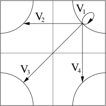
Figure 1: The anisotropic impurity scattering within the d-wave case. $V_{1}$, $V_{2}$, $V_{3}$, and $V_{4}$ are potentials for intranode, adjacent-node along the $\hat{a}$-axis direction, opposite-node, and adjacent-node impurity scattering along the $\hat{b}$-axis direction scattering.

We emphasize that the anisotropy of the impurity scattering potential (then CuO₂ plane microwave conductivity) has been reflected by this important difference between the adjacent-node impurity scattering strengths $V_{2}$ and $V_{4}$. Now we follow our previous discussions wangmicro , and obtain explicitly the $\hat{a}$-axis and $\hat{b}$-axis microwave conductivities of the ortho-II YBa₂Cu₃O_6+y as,

$$\sigma_{a}(\omega,T) = 4e^{2}v^{2}_{f}\int^{\infty}_{-\infty}{d\omega^{\prime}\over 2\pi}{n_{F}(\omega^{\prime})-n_{F}(\omega^{\prime}+\omega)\over\omega^{\prime}}[{\rm Re}J_{a}(\omega^{\prime}-i\delta,\omega^{\prime}+\omega+i\delta)-{\rm Re}J_{a}(\omega^{\prime}+i\delta,\omega^{\prime}+\omega+i\delta)],$$ (13a)

$$\sigma_{b}(\omega,T) = 4e^{2}v^{2}_{f}\int^{\infty}_{-\infty}{d\omega^{\prime}\over 2\pi}{n_{F}(\omega^{\prime})-n_{F}(\omega^{\prime}+\omega)\over\omega^{\prime}}[{\rm Re}J_{b}(\omega^{\prime}-i\delta,\omega^{\prime}+\omega+i\delta)-{\rm Re}J_{b}(\omega^{\prime}+i\delta,\omega^{\prime}+\omega+i\delta)],$$ (13b)

where $n_{F}(\omega)$ is the fermion distribution function, $v_{f}=\sqrt{2}t$ is the electron velocity at the nodal points, and the kernel function $J_{a}(\omega^{\prime},\omega)$ and $J_{b}(\omega^{\prime},\omega)$ are given by,

$$J_{a}(\omega^{\prime},\omega)={I^{(0)}_{0}+L^{a}_{1}[I^{(0)}_{0}I_{3}^{(3)}+I_{0}^{(3)}I_{3}^{(0)}]\over[1-(L^{a}_{1}I_{0}^{(0)}+L^{a}_{2}I^{(0)}_{3})][1-(L^{a}_{1}I_{3}^{(3)}+L^{a}_{2}I^{(3)}_{0})]-[L^{a}_{1}I_{0}^{(3)}+L^{a}_{2}I^{(3)}_{3}][L^{a}_{1}I_{3}^{(0)}+L^{a}_{2}I^{(0)}_{0}]},~{}~{}~{}~{}~{}$$ (14a)

$$J_{b}(\omega^{\prime},\omega)={I^{(0)}_{0}+L^{b}_{1}[I^{(0)}_{0}I_{3}^{(3)}+I_{0}^{(3)}I_{3}^{(0)}]\over[1-(L^{b}_{1}I_{0}^{(0)}+L^{b}_{2}I^{(0)}_{3})][1-(L^{b}_{1}I_{3}^{(3)}+L^{b}_{2}I^{(3)}_{0})]-[L^{b}_{1}I_{0}^{(3)}+L^{b}_{2}I^{(3)}_{3}][L^{b}_{1}I_{3}^{(0)}+L^{b}_{2}I^{(0)}_{0}]},~{}~{}~{}~{}~{}$$ (14b)

where the functions $L^{a}_{1}$, $L^{a}_{2}$, $L^{b}_{1}$, and $L^{a}_{2}$ are expressed as,

$$L^{a}_{1}(\omega^{\prime},\omega) = \rho_{i}[T_{11}^{0}(\omega^{\prime})T_{11}^{0}(\omega^{\prime}+\omega)+T_{11}^{3}(\omega^{\prime})T_{11}^{3}(\omega^{\prime}+\omega)-T_{12}^{0}(\omega^{\prime})T_{12}^{0}(\omega^{\prime}+\omega)-T_{12}^{3}(\omega^{\prime})T_{12}^{3}(\omega^{\prime}+\omega)$$ (15a)

$$- T_{13}^{0}(\omega^{\prime})T_{13}^{0}(\omega^{\prime}+\omega)-T_{13}^{3}(\omega^{\prime})T_{13}^{3}(\omega^{\prime}+\omega)+T_{14}^{0}(\omega^{\prime})T_{14}^{0}(\omega^{\prime}+\omega)+T_{14}^{3}(\omega^{\prime})T_{14}^{3}(\omega^{\prime}+\omega)],$$

$$L^{a}_{2}(\omega^{\prime},\omega) = \rho_{i}[T_{11}^{0}(\omega^{\prime})T_{11}^{3}(\omega^{\prime}+\omega)+T_{11}^{3}(\omega^{\prime})T_{11}^{0}(\omega^{\prime}+\omega)-T_{12}^{0}(\omega^{\prime})T_{12}^{3}(\omega^{\prime}+\omega)-T_{12}^{3}(\omega^{\prime})T_{12}^{0}(\omega^{\prime}+\omega)$$ (15b)

$$- T_{13}^{0}(\omega^{\prime})T_{13}^{3}(\omega^{\prime}+\omega)-T_{13}^{3}(\omega^{\prime})T_{13}^{0}(\omega^{\prime}+\omega)+T_{14}^{0}(\omega^{\prime})T_{14}^{3}(\omega^{\prime}+\omega)+T_{14}^{3}(\omega^{\prime})T_{14}^{0}(\omega^{\prime}+\omega)],$$

$$L^{b}_{1}(\omega^{\prime},\omega) = \rho_{i}[T_{11}^{0}(\omega^{\prime})T_{11}^{0}(\omega^{\prime}+\omega)+T_{11}^{3}(\omega^{\prime})T_{11}^{3}(\omega^{\prime}+i\omega)+T_{12}^{0}(\omega^{\prime})T_{12}^{0}(\omega^{\prime}+\omega)+T_{12}^{3}(\omega^{\prime})T_{12}^{3}(\omega^{\prime}+\omega)$$ (15c)

$$- T_{13}^{0}(\omega^{\prime})T_{13}^{0}(\omega^{\prime}+\omega)-T_{13}^{3}(\omega^{\prime})T_{13}^{3}(\omega^{\prime}+\omega)-T_{14}^{0}(\omega^{\prime})T_{14}^{0}(\omega^{\prime}+\omega)-T_{14}^{3}(\omega^{\prime})T_{14}^{3}(\omega^{\prime}+\omega)],$$

$$L^{b}_{2}(\omega^{\prime},\omega) = \rho_{i}[T_{11}^{0}(\omega^{\prime})T_{11}^{3}(\omega^{\prime}+\omega)+T_{11}^{3}(\omega^{\prime})T_{11}^{0}(\omega^{\prime}+\omega)+T_{12}^{0}(\omega^{\prime})T_{12}^{3}(\omega^{\prime}+\omega)+T_{12}^{3}(\omega^{\prime})T_{12}^{0}(\omega^{\prime}+\omega)$$ (15d)

$$- T_{13}^{0}(\omega^{\prime})T_{13}^{3}(\omega^{\prime}+\omega)-T_{13}^{3}(\omega^{\prime})T_{13}^{0}(\omega^{\prime}+\omega)-T_{14}^{0}(\omega^{\prime})T_{14}^{3}(\omega^{\prime}+\omega)-T_{14}^{3}(\omega^{\prime})T_{14}^{0}(\omega^{\prime}+\omega)],$$

and the functions $I^{(0)}_{0}(\omega,\omega^{\prime})$ and $I^{(0)}_{3}(\omega,\omega^{\prime})$ are evaluated in terms of the dressed Green’s function (5) as,

$$I^{(0)}_{0}(\omega,\omega^{\prime})\tau_{0} + I^{(3)}_{0}(\omega,\omega^{\prime})\tau_{3}={1\over N}\sum_{{\bf k}}\tilde{G}_{I}({\bf k},\omega)\tilde{G}_{I}({\bf k},\omega+\omega^{\prime}),$$ (16a)

$$I^{(0)}_{3}(\omega,\omega^{\prime})\tau_{0} + I^{(3)}_{3}(\omega,\omega^{\prime})\tau_{3}={1\over N}\sum_{{\bf k}}\tilde{G}_{I}({\bf k},\omega)\tilde{\tau}_{3}\tilde{G}_{I}({\bf k},\omega+\omega^{\prime}).$$ (16b)

It is clearly that if the effect of the $\hat{b}$-axis CuO chain induced impurities is neglected, i.e., $V_{2}=V_{4}$, this leads to $L_{1}^{a}(\omega^{\prime},\omega)=L_{1}^{b}(\omega^{\prime},\omega)$ and $L_{2}^{a}(\omega^{\prime},\omega)=L_{2}^{b}(\omega^{\prime},\omega)$, and then the $\hat{a}$-axis and $\hat{b}$-axis microwave conductivities in Eq. (9) are reduced to the isotropic one wangmicro $\sigma_{a}(\omega^{\prime},\omega)=\sigma_{b}(\omega^{\prime},\omega)=\sigma(\omega^{\prime},\omega)$.

III Energy and temperature dependence of the $\hat{a}$-axis and $\hat{b}$-axis microwave conductivities for the ortho-II YBa₂Cu₃O_6.50

In cuprate superconductors, although the values of $J$ and $t$ is believed to vary somewhat from compound to compound shen , however, as a qualitative discussion, the commonly used parameters in this paper are chosen as $t/J=2.5$, with an reasonably estimative value of $J\sim 1000$K. We are now ready to discuss the energy and temperature dependence of the $\hat{a}$-axis and $\hat{b}$-axis quasiparticle transport of the ortho-II YBa₂Cu₃O_6.50 with the extended anisotropy impurity scattering. We have performed a calculation for the energy dependence of the $\hat{a}$-axis and $\hat{b}$-axis microwave conductivities $\sigma_{a}(\omega,T)$ and $\sigma_{b}(\omega,T)$ in Eq. (9) at low temperatures, and the results of $\sigma_{a}(\omega,T)$ (top panel) and $\sigma_{b}(\omega,T)$ (bottom panel) as a function of energy with temperature $T=0.002J=2$K (solid line), $T=0.004J=4$K (dash-dotted line) and $T=0.008J=8$K (dashed line) under the slightly strong impurity scattering potential with $V_{1}=100J$, $V_{2}=90J$, $V_{3}=30J$, and $V_{4}=30J$ at the impurity concentration $\rho_{i}=0.00002$ for the doping concentration $\delta=0.15$ are plotted in Fig. 2 in comparison with the corresponding experimental results harris of the ortho-II YBa₂Cu₃O_6.50 (inset). It is clearly that the anisotropy of the energy evolution of the low temperature microwave conductivity of the ortho-II YBa₂Cu₃O_6.50 is qualitatively reproduced harris ; bobowski , where quasiparticle spectral weights differ by a factor of two between the $\hat{a}$-axis and $\hat{b}$-axis directions. Moreover, although the cusplike lineshapes are observed along both $\hat{a}$-axis and $\hat{b}$-axis directions as in the previous case in the non-ortho-II phase of cuprate superconductors wangmicro , the width of the $\hat{a}$-axis spectrum is significantly broadened. This broadening is only attributed to increased quasiparticle scattering arising from the CuO chain induced impurities. In comparison with our previous results for the non-ortho-II phase of cuprate superconductors wangmicro , the present results of the anisotropy therefore confirm that the CuO chain induced impurity is the dominant source of the anisotropy in the microwave conductivity spectrum of the ortho-II YBa₂Cu₃O_6.50 bobowski .

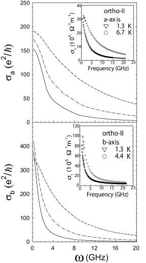
Figure 2: The microwave conductivities of the $\hat{a}$-axis (top panel) and $\hat{b}$-axis (bottom panel) as a function of energy with $T=0.002J=2$K (solid line), $T=0.004J=4$K (dash-dotted line) and $T=0.008J=8$K (dashed line) at $\rho_{i}=0.00002$ for $t/J=2.5$ with $V_{1}=100J$, $V_{2}=90J$, $V_{3}=30J$, and $V_{4}=30J$ in $\delta=0.15$. Inset: the corresponding experimental result of the ortho-II YBa₂Cu₃O_6.50 taken from Ref. harris, .

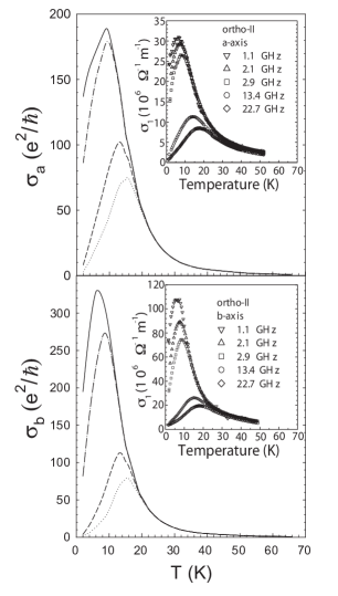
Figure 3: The microwave conductivities of the $\hat{a}$-axis (top panel) and $\hat{b}$-axis (bottom panel) as a function of temperature with energy $\omega\approx 1.14$GHz (solid line), $\omega\approx 2.28$GHz (dash-dotted line), $\omega\approx 13.4$GHz (dashed line), and $\omega\approx 22.8$GHz (dotted line) at $\rho_{i}=0.00002$ for $t/J=2.5$ with $V_{1}=100J$, $V_{2}=90J$, $V_{3}=30J$, and $V_{4}=30J$ in $\delta=0.15$. Inset: the corresponding experimental result of the ortho-II YBa₂Cu₃O_6.50 taken from Ref. harris, .

In the above discussions of the low temperature and low energy case, the inelastic quasiparticle-quasiparticle scattering process has been dropped, since it is suppressed at low temperatures and low energies due to the large SC gap parameter in the quasiparticle excitation spectrum. For a better understanding of the anisotropy in the microwave conductivity spectrum, we now turn to discuss the temperature dependence of the quasiparticle transport of the ortho-II YBa₂Cu₃O_6.50, where $T$ may approach to $T_{c}$ from low temperature side, and therefore the inelastic quasiparticle-quasiparticle scattering process should be considered nunner . The contribution from this inelastic quasiparticle-quasiparticle scattering process is increased rapidly when $T$ approaches to $T_{c}$ from low temperature side, since there is a small SC gap parameter near $T_{c}$. In particular, it has been pointed out walker that the contribution from the quasiparticle-quasiparticle scattering process to the transport lifetime is exponentially suppressed at low temperatures, and therefore the effect of this inelastic quasiparticle-quasiparticle scattering can be considered by adding the inverse transport lifetime duffy $\tau^{-1}_{{\rm inel}}(T)$ to the imaginary part of the self-energy function $\Sigma_{0}(\omega)$ in Eq. (5) as in our previous discussions wangmicro , then the total self-energy function $\Sigma^{{\rm tot}}_{0}(\omega)$ can be expressed as walker ; nunner ; wangmicro $\Sigma^{{\rm tot}}_{0}(\omega)=\Sigma_{0}(\omega)-i[2\tau_{{\rm inel}}(T)]^{-1}$, with $\tau_{{\rm inel}}(T)$ has been chosen as $[2\tau_{{\rm inel}}(T)]^{-1}=2\times 10^{4}(T-0.002)^{4}J$. Using this total self-energy function $\Sigma^{{\rm tot}}_{0}(\omega)$ to replace $\Sigma_{0}(\omega)$ in Eq. (5), we have performed a calculation for the temperature dependence of the $\hat{a}$-axis and $\hat{b}$-axis microwave conductivities $\sigma_{a}(\omega,T)$ and $\sigma_{b}(\omega,T)$, and the results of $\sigma_{a}(\omega,T)$ and $\sigma_{b}(\omega,T)$ as a function of temperature $T$ with energy $\omega=0.0000547J\approx 1.14$GHz (solid line), $\omega=0.0001094J\approx 2.28$GHz (dash-dotted line), $\omega=0.0006564J\approx 13.4$GHz (dashed line), and $\omega=0.001094J\approx 22.8$GHz (dotted line) under the slightly strong impurity scattering potential with $V_{1}=100J$, $V_{2}=90J$, $V_{3}=30J$ and $V_{4}=30J$ at the impurity concentration $\rho_{i}=0.00002$ for the doping concentration $\delta=0.15$ are plotted in Fig. 3. For comparison, the corresponding experimental results harris of the ortho-II YBa₂Cu₃O_6.50 are also plotted in Fig. 3 (inset). Obviously, the overall temperature dependence is similar to that of the temperature dependence of the microwave conductivity in the non-ortho-II phase of cuprate superconductors wangmicro , where both $\hat{a}$-axis and $\hat{b}$-axis temperature dependent microwave conductivities $\sigma_{a}(\omega,T)$ and $\sigma_{b}(\omega,T)$ increases rapidly with increasing temperatures to a broad peak, and then falls roughly linearly. In particular, this broad peak shifts to higher temperatures as the energy increased. However, the spectral width is evidently anisotropic, where the spectral width of the $\hat{a}$-axis microwave conductivity $\sigma_{a}(\omega,T)$ is larger than the corresponding value of the $\hat{b}$-axis one. Moreover, the peak position of the $\hat{a}$-axis microwave conductivity $\sigma_{a}(\omega,T)$ is located at higher temperature than the corresponding value of the $\hat{b}$-axis one, in qualitative agreement with the experimental data of the ortho-II YBa₂Cu₃O_6.50 harris ; bobowski .

In our present theory, the anisotropy of the microwave conductivity reflects directly from the electron vertex correction due to the extended anisotropy impurity scattering potential. However, it has been shown that for all scattering strength the thermal vertex correction is negligible compared to the electron one durst , therefore we expects the heat transport of the ortho-II YBa₂Cu₃O_6.50 to be CuO₂ plane isotropic. This is a unique feature of our theory that is different from the other theory Bascones in which the fermi surface is assumed to be altered and thus the heat transport may be also anisotropic. This should be verified by further experiments.

IV Summary

Within the framework of the kinetic energy driven SC mechanism, we have studied the anisotropy in the microwave conductivity spectrum recently observed harris ; bobowski in the ortho-II YBa₂Cu₃O_6.50. The ortho-II YBa₂Cu₃O_6.50 is characterized by a periodic alternative of filled and empty $\hat{b}$-axis CuO chains. The extended anisotropy impurity scattering potential results when the extended isotropy impurity scattering potential in the CuO₂ planes incorporates the $\hat{b}$-axis CuO chain induced impurity scattering potential. Based on the nodal approximation of the quasiparticle excitations and scattering processes, we have calculated the $\hat{a}$-axis and $\hat{b}$-axis microwave conductivities with the extended anisotropy impurity scattering, and reproduced the main features harris ; bobowski of the anisotropy in the microwave conductivity spectrum of the ortho-II YBa₂Cu₃O_6.50, including the intensity and lineshape of the energy and temperature dependence of the $\hat{a}$-axis and $\hat{b}$-axis microwave conductivities. Our results also confirm that the $\hat{b}$-axis CuO chain induced impurity is the main source of the anisotropy bobowski .

- (1) To whom correspondence should be addressed.
- (2) See, e.g., the review, H. Alloul, J. Bobroff, M. Gabay, and P. J. Hirschfeld, Rev. Mod. Phys. 81, 45 (2009), and references therein.
- (3) See, e.g., the review, A. Damascelli, Z. Hussain, and Z. X. Shen, Rev. Mod. Phys. 75, 473 (2003), and references therein.
- (4) P. W. Anderson, in Frontiers and Borderlines in Many Particle Physics, edited by R. A. Broglia and J. R. Schrieffer (North-Holland, Amsterdam, 1987), p. 1; Science 235, 1196 (1987).
- (5) D. A. Bonn, R. Liang, T. M. Riseman, D. J. Baar, D. C. Morgan, K. Zhang, P. Dosanjh, T. L. Duty, A. MacFarlane, G. D. Morris, J. H. Brewer, W. N. Hardy, C. Kallin, and A. J. Berlinsky, Phys. Rev. B 47, 11314 (1993).
- (6) Shih-Fu Lee, D. C. Morgan, R. J. Ormeno, D. M. Broun, R. A. Doyle, J. R. Waldram, and K. Kadowaki, Phys. Rev. Lett. 77, 735 (1996).
- (7) A. Hosseini, R. Harris, Saeid Kamal, P. Dosanjh, J. Preston, Ruixing Liang, W. N. Hardy, and D. A. Bonn, Phys. Rev. B 60, 1349 (1999).
- (8) P. J. Turner, R. Harris, Saeid Kamal, M. E. Hayden, D. M. Broun, D. C. Morgan, A. Hosseini, P. Dosanjh, G. K. Mullins, J. S. Preston, Ruixing Liang, D. A. Bonn, and W. N. Hardy, Phys. Rev. Lett. 90, 237005 (2003).
- (9) R. Harris, P. J. Turner, Saeid Kamal, A. R. Hosseini, P. Dosanjh, G. K. Mullins, J. S. Bobowski, C. P. Bidinosti, D. M. Broun, Ruixing Liang, W. N. Hardy, and D. A. Bonn, Phys. Rev. B 74, 104508 (2006).
- (10) J. S. Bobowski, P. J. Turner, R. Harris, Ruixing Liang, D. A. Bonn, and W. N. Hardy, Physica C 460-462, 914 (2007); arXiv:cond-mat/0612344.
- (11) E. Bascones, T. M. Rice, A. O. Shorikov, A. V. Lukoyanov, and V. I. Anisimov, Phys. Rev. B 71, 012505 (2005).
- (12) W. A. Atkison, Phys. Rev. B 59, 3377 (1999); Yu Lan, Jihong Qin, and Shiping Feng, Phys. Rev. B 76, 014533 (2007).
- (13) Zhi Wang, Huaiming Guo, and Shiping Feng, Physica C 468, 1078 (2008).
- (14) Shiping Feng, Phys. Rev. B 68, 184501 (2003); Shiping Feng, Tianxing Ma, and Huaiming Guo, Physica C 436, 14 (2006).
- (15) See, e.g., the review, Shiping Feng, Huaiming Guo, Yu Lan, and Li Cheng, Int. J. Mod. Phys. B 22, 3757 (2008).
- (16) See, e.g., the review, C. C. Tsuei and J. R. Kirtley, Rev. Mod. Phys. 72, 969 (2000).
- (17) Shiping Feng, Jihong Qin, and Tianxing Ma, J. Phys. Condens. Matter 16, 343 (2004).
- (18) Huaiming Guo and Shiping Feng, Phys. Lett. A 361, 382 (2007).
- (19) A. C. Durst and P. A. Lee, Phys. Rev. B 62, 1270 (2000).
- (20) Tamara S. Nunner and P. J. Hirschfeld, Phys. Rev. B 72, 014514 (2005).
- (21) D. Duffy, P. J. Hirschfeld, and D. J. Scalapino, Phys. Rev. B 64, 224522 (2001).
- (22) S. Graser, P. J. Hirschfeld, and L. Y. Zhu, Phys. Rev. B 76, 054516 (2007).
- (23) M. B. Walker and M. F. Smith, Phys. Rev. B 61, 11285 (2000).