Origin of branch points in the spectrum of PT-symmetric periodic potentials
Abstract
There exists multiple branch points in the energy spectrum for some PT-symmetric periodic potentials, where the real eigenvalues turn into complex ones. By studying the transmission amplitude for a localized complex potential, we elucidate the physical origin of the breakdown of perturbation method and Born approximation. Mostly importantly, we derive an analytic criteria to determine why, when and where the bifurcation will occur.
pacs:
03.65.Ge, 03.65.Nk, 11.30.ErI INTRODUCTION
Non-Hermitian (NH) quantum mechanics (QM) has been used to describe an open system because complex eigenenergies imply the existence of a sink or source for the particle. The PT-symmetric hamiltonian is a special case in NHQM that can exhibit entirely real spectrapt1 . Its development has gone through various stagespt2 with applications ranging from quantum cosmology16 , quantum field theory19 to quantum computationbrach1 ; brach2 . A flourishing example is in connection with the optical lattice which can be simulated by the Schrödinger equation. This provides a fertile ground to test the NH-related concepts experimentally. In this spirit scientists have studied the PT-symmetric periodic potentials and investigated several interesting features: (1) The existence of several branch points which demarcate the real and complex spectradorey . (2) Optical soliton solutions are found within the energy gap with real eigenvaluessoliton . (3) A quantum phase transition is identified when a sufficiently large real periodic potential is superimposed to render all the spectrum realbeam . The latter two, which provide the basis for the fruitful beam dynamicssoliton ; beam , are closely related to the branch point and bifurcation feature. Although the branch points and a complex spectrum have been attributed to the failure of perturbation expansionvisual , we believe it is worthwhile to study in more detail the physical origin of this failure.
We shall start by studying a localized imaginary potential before embarking on the more interesting periodic case. Several new features are discussed in Section II which include (1) Existence of an upper bound for the imaginary part of eigenenergies. (2) Breakdown of the Born approximation for scattering states unless a large enough real potential is added. (3) Fano resonance within the imaginary barrier can cause the transmission amplitude to become huge by repetitive enhancements. (4) An incoming wave packet will also exhibit special features when its momentum is near the resonance. We find that the size of the transmission amplitude is the key to features (2) and (3). In Section III we argue that the spectrum of the PT-symmetric periodic potential is predominantly shaped by the transmission amplitude for a single unit cell. Therefore, the conclusions in Section II for a localized potential are still applicable in the periodic case. By use of the Bloch’s theorem, we derive an analytic criteria for the occurrence of branch point and the band structure bifurcation. Discussions and conclusions are arranged in the final Section IV.
II SINGLE IMAGINARY SQUARE POTENTIAL
II.1 Localized states
At first glance, one might think that the eigenenergies of a complex potential are most likely also complex. This is in fact not true. For instance, take an imaginary square potential from to where and zero potential elsewhere. It exhibits both real/imaginary eigenvalues, which are continuous/discrete and correspond to scattering/localized states, respectively.
Since the barrier potential is symmetric with respect to , the spatial part of the localized wavefunction, where has been set to unity for convenience, can be expressed as:
| (1) |
where momentum and are real and positive, is complex, and the sign denotes respectively the even/odd-parity state with respect to . The minus sign in the exponent of is to prevent it from blowing up at . These momenta are related by the complex energy :
| (2) |
One should be aware that the standard concept of density current need not survivept-sq3 the transition to NHQM. For instance, in the case of a PT-symmetric potential has to be redefined as in order to obtain the continuity equation. For the sake of arguments, let us stick to the standard notion and deduce the following mathematical equation from the Schrödinger equation for a general complex potential :
| (3) |
where the symbol Im denotes taking the imaginary part and . Integrating over the whole space gives
| (4) |
where vanishes at for the localized state in Eq.(1). This leads to the following inequality
| (5) |
which tells us that the height of the imaginary barrier serves as an upper bound for :
| (6) |
By matching the boundary conditions, we can further show that the number of these localized states is finite and their energies are discrete. In contrast to being zero for a real well, the current density is not only nonvanishing, but also quantized for an imaginary barrier/well:
| (7) |
where labels these discrete localized states.
All the derivations so far are based on the assumption that . However, it is easy to generalize to an imaginary well. The action of changing the potential from to is equivalent to reversing the time, which transforms the hydrant-like bound state into a sink. The same conclusion applies to the eigenfunctions and eigenenergies after we take the complex conjugate of the time-independent Schrödinger equation. As a result, the upper bound in Eq.(6) needs to be modified as
| (8) |
II.2 Scattering states
Another interesting problem is to study the transmission and reflection coefficients for a complex square barrier. This is relevant to our discussion of the spectrum for a periodic potential in Section III. The scattering state takes the form:
| (12) |
where subscript is to distinguish this right-moving state from its degenerate state that travels in the opposite direction. Fitting the boundary conditions, we find
| (13) | |||
| (14) |
where is the complex momentum inside the barrier. The amplitude in Eq.(12) consists of contributions from all paths that reflect inside the barrier arbitrary number of times:
| (15) |
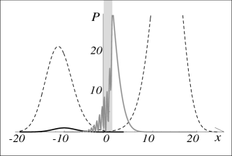
where / denote the transmission/reflection amplitudes at the boundaries and , respectively. The higher-order terms in Eq.(15) converge to zero for a real barrier. But this is no longer true for a positive imaginary barrier because the longer they stay in the source the more probability they can gain. As a result, the values of resonance peaks can be much bigger than unity, and the Born approximation that neglects the higher-order terms is expected to break down. These two features are clearly shown in Fig.1 and the number of resonances and their peak values increase when we raise in Fig.2.


Another important issue of the scattering process is the interference condition for Fano resonance. In real barriers, the resonance in transmission results from the constructive interference between different scattering paths shown in Eq.(15), which gives the familiar condition . In the mean time, reflection peaks are attributed to the destructive interference when
| (16) |
is satisfied. These two conditions become more complicated for an imaginary potential because the phase shift due to reflections from the boundaries between the imaginary and real potential regimes is energy-dependent. The amplitude in Eq.(15) can be determined by studying the reflection by an imaginary step potential of height :
| (19) |
which shows that there is an additional phase shift ranging from 0 to as increases. It is straightforward to write down an equation similar to Eq.(15) for the reflection amplitude, . Since both equations are geometric series with the same common ratio, , it is expected that the transmission and reflective resonances for an imaginary barrier should all follow the same second criterion, Eq.(16), at the limit . To verify these interference features, a partial list of the energies, peak values of the transmission coefficient and corresponding in Fig.2 are numerically calculated and summarized in Tab. 1. For an imaginary well, Eq.(19) remains valid after is replaced by . However, the resonance peaks are no longer pronounced because the sink now draws in probability as the wave reflects in the well.
| 223.6 | 257.4 | 294.1 | 333.4 | |
|---|---|---|---|---|
| 247.5 | 2322.5 | 24485.9 | 1507.7 | |
| 13.52 | 14.49 | 15.48 | 16.47 |
In order to facilitate the discussion of a PT-symmetric periodic potential in Section III, let us put the square barrier and well side by side to form a simple PT-symmetric potential. The perturbation expansion can be shown to still break down as in the periodic casebeam . The similarity goes further that the perturbation in both potentials can be salvaged by incorporating a big-enough real potential. On the other hand, we can ask how strong a complex potential can ruin the perturbation expansion. Take this pair of square barrier and well potential, , for example. The threshold for is determined when the maximum of the common ratio in Eq.(15) equals ; namely,
| (20) |
where
| (21) |
For the parameters , and , this critical equals . Numerical calculations show that this is the same threshold for the transmission amplitude to exceed 1, which shall be proved in Section III to be the harbinger for the bifurcation of specturm for the PT-symmetric periodic potential.
II.3 Evolution of a wave packet through the imaginary barrier
When a wave packet impinges on a real potential barrier, the resonances are not critical to its evolution since their transmission amplitude is of the same order as the nonresonant ones. However, as is shown in Tab. 1, the resonant amplitudes can reach a few tens of a thousand for an imaginary barrier. It is, therefore, of interest to study how a wave packet progresses through such a potential.
As usual, we first decompose it into the scattering states in Eq.(12) and the localized states in Eq.(1):
| (22) |
where the superscript denotes the right eigenstate. This is similar to the case of nonHermitian matrices, for which the right and left eigenstates may not be the same. Since they can exhibit different physical properties and time evolution, it is important to distinguish them. Take the imaginary square potential, for instance. The barrier seen by the right eigenstates in Eqs.(12) and (1) will turn into a well for their left counterparts, which are defined by
| (23) |
or
| (24) |
when expressed in the real space. These two eigenstates obey the following orthogonality relation
| (25) |
By use of the above relation and the general product, c method, introduced by Gilary et al.evolve , the weightings , in Eq.(22) can be determined as
| (26) |
The initial wave packet, , is chosen as a harmonic coherent state:
| (27) |
where and denote the position and momentum of the center of the packet, while is its mean width. For an imaginary square barrier of height , the evolution of wave packet is illustrated in Fig.3 with and chosen to be near one of the resonance peaks in Fig.1. It can be seen that the amplitude gets enhanced upon entering the imaginary barrier due to the resonance. The oscillatory behavior only exists at intermediate time, as depicted by the gray line. As the wave packet exits the barrier, the amplitudes of both transmitted and reflected waves have already been enhanced by and times each.
III PT-SYMMETRIC PERIODIC POTENTIAL
III.1 Origin of bifurcation
In the following, we generalize the single imaginary potential to a PT-symmetric periodic one. Set the unit cell in and denote the eigenfunction by
| (28) |
where and are the right- and left-moving scattering states in the unit cell similar to Eq.(12). According to the Bloch’s theorem, the wavefunction in its previous cell can be represented as:
| (29) |
where is the Bloch wave number. Matching the boundary conditions at gives
| (30) |
where denotes . By use of the equality , the above equations require the following condition in order to have a nonzero :
| (31) |
where
and the definition of is similar but with the subindices and interchanged. Equation (31) gives us the dispersion relation for the spectrum.
Let us write down the form of at explicitly
| (34) | |||
| (37) |
where the amplitudes may vary with . Inserting them in Eq.(31) gives the relation between the energy and for a general periodic potential:
| (38) |
The fact that we are interested at the branch points of PT-symmetric periodic potentials allows us to further simplify Eq.(38). First, take the complex conjugate of the Schrödinger equation for
| (39) |
If we choose the unit cell to also exhibit the PT-symmetry, the potential will become identical to . Furthermore, is the same as since the eigenenergy is real at the branch point. These two properties combined with Eq.(39) tell us that must be a linear combination of the two scattering states:
| (40) |
This relation gives four equations, each of which corresponds to matching the right- and left-moving part of the wavefunctions on either side of the unit cell: , , and . It is straightforward to show that they yield which simplifies Eq.(38) to:
| (41) |
where is the phase of . If should ever be larger than 1 near the extrema of the LHS in Eq.(41), there will be no real solution for those that make large. In other words, the eigenenergies near the Brillouin zone boundaries of are sure to be complex. We emphasize that the condition that exceeds unity for some alone is not enough to predict the bifurcation. It has to coincide with the occurrence of extreme values for . This is complement to the previous conclusionvisual that perturbation forbids bifurcation. What we have shown here is that guarantees there will be no bifurcation. It is then natural to ask whether implies the validity of perturbation. As far as the PT-symmetric periodic square potential in the next subsection is concerned, this statement has been checked to hold in Section II(B).
III.2 PT-symmetric periodic square potential
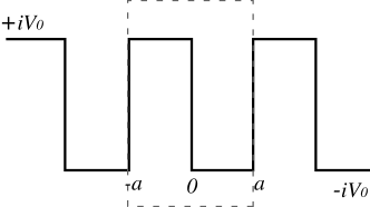
As a demonstration, we quantify our conclusions in the previous subsection for the special case of a PT-symmetric periodic square potential, as shown in Fig.4. The transimission coefficient for the unit cell can be calculated as:
| (42) |
where and represents the momentum in the imaginary barrier/well region. The transmission and reflection amplitudes corresponding to the three boundaries are denoted by , , , and .
Inserting Eq.(42) into Eq.(41) and the dispersion relation can be determined as:
| (43) |
The band structure is solved numerically and plotted in Fig.5.
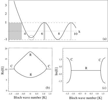
The perturbation method has been demonstrated to break down for a single localized complex barrier potential in Section II(B), either with or without an accompanying well. When it is generalized to a PT-symmetric periodic potential, we are sure that the perturbation remains at fault from the analysis within one unit cell. In the meantime, Fig.5 shows that the originally real eigenenergies evolve into both complex and real spectra. So the existence of branch points and the breakdown of perturbation are tied together as proved by Ref.visual . In the mean time, the values of at these extrema also become greater than unity, as is shown in Tab.2.
In passing, we observed a special bond between the branch points and the Fano resonances discussed in Section II(B). Since the momenta and here happen to be complex conjugates when is real, the reflection amplitude in Eq.(19) is rendered pure imaginary. The condition for constructive interference becomes identical to Eq.(16). This is supported by the numerical results for the branch points presented in Tab.2, which indeed approach those for the resonances.
| 10.39 | 30.62 | 60.34 | 99.87 | |
|---|---|---|---|---|
| 1.36 | 1.02 | 1.00 | 1.00 | |
| 1.50 | 2.50 | 3.50 | 4.50 |
IV DISCUSSIONS AND CONCLUSIONS
Since the non-Hermitian potential results from our examining an open system which is allowed to exchange particles with its environment, the conventional continuity equation is no longer obeyedpt-sq1 ; pt-sq3 ; non-unitarity1 ; non-unitarity2 . One interesting debatelocalize is whether it is meaningful to mend this loss of unitarity. Several studieslocalize ; delta-perturb ; zno have been devoted to this effort. They tried to construct a metric and corresponding transformed wave function as the general frameworkn1 ; n2 ; np1 ; np2 ; np3 to examine the subsystem in a quasi-Hermitian analysis. Although the unitarity can be restored, one is constrained to discuss wavefunctions either coming simultaneously from both sideslocalize ; delta-perturb or exhibiting different normalization constants on either side of the potentialzno . To resolve these dilemmas, Jonesdelta-perturb suggested that one simply treats the non-Hermitian scattering potential as an effective one in the standard framework of quantum mechanics. This is the view we adopt in this work at studying the localized NH potentials as a phenomenological model of a quantum sink or source in an open system.
In conclusion, although the breakdown of perturbation approach has been identified to be intimately linked to the existence of complex spectrum for a PT-symmetric periodic potential, we offer new insights into their relationship by studying the less sophisticated case of an imaginary barrier potential. Due to the simplicity of this potential form, we are able to elucidate the cause of the similar breakdown of perturbation, why the perturbation can be remedied by the superimposition of a sufficiently large real potential, and the condition for a constructive interference which differs from that for a real potential. Most importantly, we provide a more comprehensive criteria through Eq.(41) on why, when and where the bifurcation will occur.
We thank Hsiu-Hau Lin for useful comments and acknowledge the support by NSC in Taiwan under grant No. 95-2112-M007-046-MY3.
References
- (1) C. M. Bender and S. Boettcher, Phys. Rev. Lett. 80, 5243 (1998).
- (2) C. M. Bender, Contemp. Phys. 46, 277 (2005).
- (3) A. Mostafazadeh, Ann. Phys. (N.Y.) 309, 1 (2004).
- (4) C. M. Bender, Rep. Prog. Phys. 70, 947 (2007).
- (5) C. M. Bender, D. C. Brody, H. F. Jones, and B. K. Meister, Phys. Rev. Lett. 98, 040403 (2007).
- (6) A. Mostafazadeh, Phys. Rev. Lett. 99, 130502 (2007).
- (7) P. Dorey, C. Dunning, and R. Tateo, J. Phys. A: Math. Gen. 34, 5679 (2001).
- (8) Z. H. Musslimani, K. G. Makris, R. El-Ganainy, and D. N. Christodoulides, Phys. Rev. Lett. 100, 030402 (2008).
- (9) K. G. Makris, R. El-Ganainy, and D. N. Christodoulides,and Z. H. Musslimani, Phys. Rev. Lett. 100, 103904 (2008).
- (10) S. Klaiman, U. Günther, and N. Moiseyev, Phys. Rev. Lett. 101, 080402 (2008).
- (11) F. Cannata, J-P. Dedonder, and A. Ventura, Ann. Phys. (N.Y.) 322, 397 (2007).
- (12) I. Gilary, A. Fleischer, and N. Moiseyev, Phys. Rev. A. 72, 012117 (2005).
- (13) Z. Ahmed, Phys. Lett. A. 324, 152 (2004).
- (14) Z. Ahmed, C. M. Bender, and M. V. Berry, J. Phys. A: Math. Gen. 38, L627 (2005).
- (15) M. Znojil, J. Phys. A: Math. Gen. 39, 13325 (2006).
- (16) H. F. Jones, Phys. Rev. D. 76, 125003 (2007).
- (17) H. F. Jones, Phys. Rev. D. 78, 065032 (2008).
- (18) M. Znojil, Phys. Rev. D. 78, 025026 (2008).
- (19) C. M. Bender, D. C. Brody, and H. F. Jones, Phys. Rev. Lett. 89, 270401 (2002); ibid. 92, 119902(E) (2004).
- (20) A. Mostafazadeh, J. Math. Phys. (N.Y.) 43, 205 (2002).
- (21) H. F. Jones, J. Phys. A: Math. Gen. 38, 1741 (2005).
- (22) A. Mostafazadeh, J. Phys. A: Math. Gen. 38, 6557 (2005); ibid. 38, 8185(E) (2005).
- (23) H. F. Jones and J. Mateo, Phys. Rev. D 73, 085002 (2006).