Rouse Modes of Self-avoiding Flexible Polymers

Abstract

Using a lattice-based Monte Carlo code for simulating self-avoiding flexible polymers in three dimensions in the absence of explicit hydrodynamics, we study their Rouse modes. For self-avoiding polymers, the Rouse modes are not expected to be statistically independent; nevertheless, we demonstrate that numerically these modes maintain a high degree of statistical independence. Based on high-precision simulation data we put forward an approximate analytical expression for the mode amplitude correlation functions for long polymers. From this, we derive analytically and confirm numerically several scaling properties for self-avoiding flexible polymers, such as (i) the real-space end-to-end distance, (ii) the end-to-end vector correlation function, (iii) the correlation function of the small spatial vector connecting two nearby monomers at the middle of a polymer, and (iv) the anomalous dynamics of the middle monomer. Importantly, expanding on our recent work on the theory of polymer translocation, we also demonstrate that the anomalous dynamics of the middle monomer can be obtained from the forces it experiences, by the use of the fluctuation-dissipation theorem.

I Introduction

Polymer dynamics is a field where first-principle analytical derivations of most quantities of interest from microscopic monomeric movements are difficult to come by. Indeed, the answer to the question why phantom polymers (theoretical realizations of polymers that can intersect themselves) remain, to this day, the central pillar for studying polymer dynamics is easily traced to the fact that they allow full analytical calculations of essentially all of their dynamical properties. In the absence of explicit hydrodynamics, a phantom polymer’s dynamics is described by the so-called Rouse equation that forms the basis of all analytical calculations doi ; de . The Rouse equation holds in the high-viscosity limit of the surrounding medium, and the dynamics of the monomers are “overdamped”, i.e., the velocity of each monomer at any given time is proportional to the total force it experiences. In the Rouse equation the total force in any monomer is comprised of the spring forces due to its neighboring monomers, and the random thermal forces from the surrounding medium. The linearity of the Rouse equation allows one to decompose it into linear dynamical equations of independently evolving (Rouse) modes, which are the Fourier transforms of the monomer co-ordinates in three dimensional space. In detail, we consider a polymer of length $N$, consisting of $N+1$ monomers connected sequentially by $N$ bonds (harmonic springs). The positions $\vec{R}_{n}(t)$ of monomers $n=0,\ldots,N$ at time $t$ can then undergo Fourier transformation, yielding for the amplitude of the $p$-th mode ($p$ is an integer $\geq 0$)

$$\vec{X}_{p}(t)=\frac{1}{N+1}\sum_{n=0}^{N}\cos\left[\frac{\pi(n+1/2)p}{N+1}\right]\,\vec{R}_{n}(t).$$ (1)

The cornerstone of all analytical calculations for phantom polymer dynamics is the following relation for $p,q\neq 0$, derived exactly from the Rouse equation:

$$X_{pq}(t)=\langle\vec{X}_{p}(t)\cdot\vec{X}_{q}(0)\rangle\propto\frac{N}{p^{2}}\,\exp\left[-A\,\frac{p^{2}}{N^{2}}\,t\right]\,\delta_{pq},$$ (2)

where $\delta_{pq}$ is the Kronecker delta function, and $A$ a constant. All throughout this paper, the angular brackets represent an average over the equilibrium ensemble of polymers. Equation (2) is further supplemented by $X_{0p}(t)=0$ for $p\neq 0$, and $X_{00}(t)=m\delta(t)$, where $\vec{X}_{0}(t)$ is the location of the center-of-mass of the polymer at time $t$, and $m\propto 1/N$ is the mobility of the center-of-mass of the polymer. The Kronecker delta terms signify the statistical independence of the modes of a phantom polymer. Using these mode amplitude correlation functions, the quantities of interest for a phantom polymer can be analytically tracked by reconstructing them from the modes doi ; de . However, in reality, a polymer is not phantom, but is self-avoiding. The self-avoidance property introduces long-range correlations along the backbone of the polymer, and it destroys the linearity of the Rouse equation, making a similar [to Eq. (2)] equation for the mode amplitude correlation functions impossible to derive from the appropriately formulated Rouse equation. Because of this reason, it comes as no surprise to us that for self-avoiding polymers we have not been able to find, in published literature, a comprehensive study of the mode amplitude correlations that connects to the scaling properties of self-avoiding polymers.

The purpose of this paper is to put forward an approximate analytical expression for the mode amplitude correlation functions for long polymers, which is then corroborated with extensive simulations of a lattice-based model for the dynamics of self-avoiding flexible polymers in three dimensions in the absence of explicit hydrodynamics. To be more precise, with $\nu\approx 0.588$ (the Flory exponent in three dimensions), and $A_{1}$ and $A_{2}$ two constants, we demonstrate that for a self-avoiding Rouse polymer of length $N$

$$X_{pq}(t)=\langle\vec{X}_{p}(t)\cdot\vec{X}_{q}(0)\rangle\approx A_{1}\,\frac{N^{2\nu}}{p^{1+2\nu}}\,\exp\left[-A_{2}\,\frac{p^{1+2\nu}}{N^{1+2\nu}}\,t\right]\,\delta_{pq}$$ (3)

for $p,q\neq 0$ holds up to a very good approximation for long polymers, while $X_{0p}(t)=0$ for $p\neq 0$ and $X_{00}(t)\propto(1/N)\delta(t)$ holds exactly. The reasons why Eq. (3) is not exact are the following: (a) although numerically the modes maintain a high degree of statistical independence, the mode amplitude correlation functions are not exactly statistically independent (we do not expect to be so anyway); and (b) for higher modes ($p,q\gtrsim 6$) there are small deviations from exponential behavior at long times. Nevertheless, given that $X_{pp}(0)$ is a rapidly decaying function of $p$, the dominant contribution of the modes to quantities of interest for the polymer at long time-scales come from the lower modes. As a result, such quantities can be analytically reconstructed from Eq. (3). We demonstrate this by using Eq. (3) to derive several scaling properties for self-avoiding polymers, such as (i) the real-space end-to-end distance, (ii) the end-to-end vector correlation function, (iii) the correlation function of the small spatial vector connecting two nearby monomers at the middle of the polymer, and (iv) the anomalous dynamics of the middle monomer. Some of these scaling laws can also be obtained from the dynamic scaling law doi . Note that except the case for characterizing the anomalous dynamics of the middle monomer, all the other quantities (as above) concern only the polymer’s internal structure; implying that for (i-iii) we only need Eq. (3), while for the anomalous dynamics of the middle monomer we also need $X_{00}(t)$ and $X_{0p}(t)$ for $p\neq 0$. Note also that the standard Rouse result Eq. (2) is recovered when we simply replace $\nu$ by $1/2$ for a phantom polymer. Apparently, the dominant consequence of volume exclusion is the different size scaling of the self-avoiding chains. The inability for polymers to cross each other does not seem to cause large cross-correlations between different modes. Thus, given the content of this paper, we expect that Eq. (3) will provide researchers a way forward for analytical treatment of the properties of self-avoiding polymers.

The structure of this paper is as follows. In Sec. II we describe our polymer model and demonstrate the scaling property Eq. (3). In Sec. III we use Eq. (3) to obtain the scaling properties for the real-space end-to-end distance and the end-to-end vector correlation function. In Sec. IV we derive the scaling properties of the small spatial vector connecting two nearby monomers. In Sec. V we derive the anomalous dynamics of the middle monomer, and by expanding our recent work on the theory of polymer translocation, show that the anomalous dynamics of the middle monomer can also be obtained by using the fluctuation-dissipation theorem. Our conclusions are then summarized in Sec. VI.

II Our polymer model and the scaling properties of the mode amplitude correlation functions

II.1 Our polymer model and the calculation of the mode amplitudes

Over the last years, we have developed a highly efficient simulation approach to polymer dynamics. This is made possible via a lattice polymer model, based on Rubinstein’s repton model rubinstein for a single reptating polymer, with the addition of sideways moves (Rouse dynamics). A detailed description of this model, its computationally efficient implementation and a study of some of its properties and applications can be found in Refs. heukelum03 ; LatMCmodel .

In this model, each polymer is represented by a sequential string of monomers, living on a face-centered-cubic lattice with periodic boundary conditions in all three spatial directions. Monomers adjacent in the string are located either in the same, or in neighboring lattice sites. The polymers are self-avoiding: multiple occupation of lattice sites is not allowed, except for a set of adjacent monomers. The polymers move through a sequence of random single-monomer hops to neighboring lattice sites. These hops can be along the contour of the polymer, thus explicitly providing reptation dynamics. They can also change the contour “sideways”, providing Rouse dynamics. Each kind of movement is attempted with a statistical rate of unity, which provides us with the definition of time. This model has been used before to simulate the diffusion and exchange of polymers in an equilibrated layer of adsorbed polymers klein_adsorbed . Recently, we have used this code extensively to study polymer translocation under a variety of circumstances wolterink06 ; trans1 ; trans2 ; trans3 ; trans3a ; vocks08 , and also to study the dynamics of polymer adsorption adsorb .

Given that our model has periodic boundary conditions in all three spatial directions, we use the following definition for the mode amplitude:

$$\vec{X}_{p}(t)=\frac{1}{N+1}\sum_{n=0}^{N}[\vec{R}_{n}(t)-\vec{R}_{0}(t)]\cos\left[\frac{\pi(n+1/2)p}{N+1}\right],$$ (4)

where $\vec{R}_{0}(t)$ is the location of the zero-th monomer at time $t$. In this definition we only need the spanning vectors, i.e., monomer co-ordinates w.r.t. that of monomer zero. These spanning vectors are obtained from a summation over the bond vectors between monomers adjacent in the string. This completely avoids the invocation of periodic images, and allows for spanning distances which exceed half the box size. Note that Eq. (4) can be derived from Eq. (1) as follows. First we use

$$\frac{1}{N+1}\sum_{n=0}^{N}\cos\left[\frac{\pi(n+1/2)p}{N+1}\right]\,\cos\left[\frac{\pi(n+1/2)p^{\prime}}{N+1}\right]=\frac{1}{2}\,\delta_{p,p^{\prime}},$$ (5)

in order to express $\vec{R}_{n}(t)$, the location of the $n$-th monomer w.r.t. that of the center-of-mass $\vec{R}_{cm}(t)\equiv\vec{X}_{0}(t)$, from the inverse Fourier transform of Eq. (1), as

$$\vec{R}_{n}(t)=\vec{R}_{cm}(t)+2\sum_{p=1}^{\infty}\vec{X}_{p}(t)\,\cos\left[\frac{\pi(n+1/2)p}{N+1}\right].$$ (6)

Then we write

$$\vec{R}_{0}(t)=\vec{R}_{cm}(t)+2\sum_{p=1}^{\infty}\vec{X}_{p}(t)\,\cos\left[\frac{\pi p}{2(N+1)}\right],$$ (7)

i.e.,

$$\vec{R}_{n}(t)-\vec{R}_{0}(t)=2\sum_{p=1}^{\infty}\vec{X}_{p}(t)\,\left\{\cos\left[\frac{\pi(n+1/2)p}{N+1}\right]-\cos\left[\frac{\pi p}{2(N+1)}\right]\right\},$$ (8)

from which Eq. (4) follows with the use of Eq. (5). Equation (4) shows that the modes $q\neq 0$ relate only to the polymers’ structural configuration, as remarked earlier.

II.2 The scaling properties of the mode amplitude correlation functions

We start with the behavior of $X_{00}(t)$. We note that the internal forces over the entire polymer at any time sum to zero, and therefore, (for the overdamped dynamics in the Rouse model) the motion of its center-of-mass is simply proportional to the average thermal fluctuating force on the entire polymer. This force is $\delta$-correlated in time, which implies that the center-of-mass of the polymer simply performs a random walk. In fact, $X_{00}(t)=m^{\prime}\delta(t)$, and the mobility $m^{\prime}\propto 1/N$. This leads us to the result that $X_{00}(t)\propto(1/N)\delta(t)$. We will return to the motion of the center-of-mass in Sec. V.

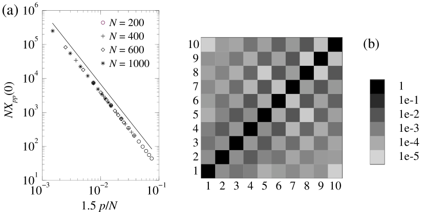
Figure 1: (a) The scaling $X_{pp}(0)\sim N^{2\nu}/p^{1+2\nu}$ demonstrated for $p=1,\ldots,10$ for $N=200$, 400, 600 and 1000. The solid line corresponds to $NX_{pp}(0)\sim(N/p)^{-(1+2\nu)}\approx(N/p)^{-2.176}$. (b) The matrix $\chi_{pq}(0)\equiv X_{pq}(0)/\sqrt{X_{pp}(0)C_{qq}(0)}$ in logarithmic grayscale for $p,q=1,\ldots,10$ for $N=1000$ in a square checkerboard plot. See text for details.

Next, for the behavior of $X_{0p}(t)$ for $p\neq 0$ we proceed as follows. We note that $X_{0p}(0)=0$. Indeed, $X_{0p}(0)$ is the equilibrium average over the dot product of $\vec{X}_{0}$ and $\vec{X}_{p}$ at zero time difference, for which, for any given value of $\vec{X}_{p}$, the center-of-mass is equally likely to be present at any location within the periodic box. For the calculation of $X_{0p}(t)$, having summed over all the locations of $\vec{X}_{0}$ for a given value of $\vec{X}_{p}$ at the first step, and then having summed over the configurations $\vec{X}_{p}$ at the second step, we obtain $X_{0p}(0)=0$ (from the first step). Thereafter, we use the result that the center-of-mass performs a simple random walk, further implying that $X_{0p}(t)=X_{0p}(0)$, which equals zero.

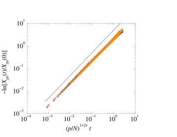
Figure 2: Data collapse for $-\ln[X_{pp}(t)/X_{pp}(0)]$ as a function of $(p/N)^{1+2\nu}t$, for $p=1$ (stars), 2 (triangles down), 3 (crosses), 4 (triangles up), 5 (diamonds), 6 (pluses), 7 (circles), and $N=200$ (red), 400 (blue), 600 (green) and 1000 (orange). The collapsed data are fitted well with an exponential; however, we note that there are small (but systematic) deviations from the exponential behavior for $p>>1$. The solid (black) line corresponds to $-\ln[X_{pp}(t)/X_{pp}(0)]\sim(p/N)^{1+2\nu}t$.

Finally, we demonstrate the scaling property of $X_{pq}(t)$ for $p,q\neq 0$ in Figs. 1 and 2. In Fig. 1(a) we present the data for $p=1,\ldots,10$ for $N=200$, 400, 600 and 1000, and demonstrate that $X_{pp}(0)\sim N^{2\nu}/p^{1+2\nu}$ up to a high precision. In Fig. 1(b) we plot the matrix $\chi_{pq}(0)\equiv X_{pq}(0)/\sqrt{X_{pp}(0)X_{qq}(0)}$ in logarithmic grayscale for $p,q=1,\ldots,10$ for $N=1000$, wherein the diagonal elements are unity by construction. The off-diagonal elements of $\chi_{pq}(0)$ are typically three or more orders of magnitude smaller than the diagonal ones. Cross-correlations between two even or between two odd modes are strictly not zero. Cross-correlations between even and odd modes are much smaller, and it is likely that these are also strictly not zero, but we cannot ascertain that within our numerical precision. We emphasize that the off-diagonal elements of $\chi_{pq}(0)$ not being zero is not caused by the lack of numerical precision, or is due to artifacts of our model — similar features have been found in Ref. downey for single polymers, and in Ref. binder for polymer melts; the modes are simply not statistically independent for self-avoiding polymers. Nevertheless, the precision with which the modes remain statistically independent is remarkable.

In Fig. 2 we plot $-\ln[X_{pp}(t)/X_{pp}(0)]$ as a function of $(p/N)^{1+2\nu}t$ for $p=1,\ldots,7$, and $N=200$, 400, 600 and 1000, and obtain a data collapse. The collapsed data are well fitted by an exponential behavior of $X_{pp}(t)/X_{pp}(0)$; however, we note that there are small (but systematic) deviations from the exponential behavior for $p\gtrsim 6$. These deviations are larger for larger $p$, although this fact is not very clearly discernible in Fig. 2.

As remarked before Eq. (3), Figs. 1 and 2 collectively demonstrate that the scaling behavior Eq. (3) is not exact; instead, it is a rather good approximation. In the following sections we will use the approximate scaling behavior of Eq. (3) and demonstrate that it reproduces the scaling behavior of several observables for self-avoiding polymers.

III Scaling of the end-to-end distance and the end-to-end vector correlation function

In order to calculate the equilibrium end-to-end distance we use Eq. (8) and write

$$\vec{R}_{N}(t)-\vec{R}_{0}(t)=2\sum_{p=1}^{\infty}\vec{X}_{p}(t)\,\left\{\cos\left[\frac{\pi(N+1/2)p}{N+1}\right]-\cos\left[\frac{\pi p}{2(N+1)}\right]\right\},$$ (9)

from which, using the scaling relation (3) we extract

$$\langle[\vec{R}_{N}(t)-\vec{R}_{0}(t)]^{2}\rangle\approx 16A_{1}N^{2\nu}\sum_{p\,\in\,\text{\scriptsize odd}}\frac{1}{p^{1+2\nu}}\,\sin^{2}\left[\frac{\pi Np}{2(N+1)}\right]$$ (10)

$$=16A_{1}N^{2\nu}\sum_{p\,\in\,\text{\scriptsize odd}}\frac{1}{p^{1+2\nu}}\,\left\{1-\sin^{2}\left[\frac{\pi p}{2(N+1)}\right]\right\}.$$

On the r.h.s. of Eq. (10) the first term $\displaystyle{\sum_{p\,\in\,\text{\scriptsize odd}}p^{-(1+2\nu)}}$ sums up to a numerical constant, and the second term $\displaystyle{\sum_{p\,\in\,\text{\scriptsize odd}}p^{-(1+2\nu)}\sin^{2}[\pi p/2(N+1)]}$ can be converted to an integral

$$8A_{1}\int_{0}^{\infty}dx\,\frac{\sin^{2}[\pi x/2]}{x^{1+2\nu}}$$

with an integrable singularity at $x=0$. The first term produces the well-known Flory scaling behavior $\langle[\vec{R}_{N}(t)-\vec{R}_{0}(t)]^{2}\rangle\sim N^{2\nu}$, while the second term provides a correction of $O(1)$ to the scaling which can be neglected in the scaling limit.

The end-to-end vector correlation function can be similarly expressed in terms of the mode amplitude correlation functions; however, in order to obtain its scaling behavior we do not need to do so. The point is that at long times the dominant contribution of the end-to-end vector comes from the mode $p=1$, and thus the approximate scaling (3) confirms that the end-to-end vector correlation function decays exponentially in time, for which the characteristic time for the decay is given by the Rouse time $\tau_{R}\sim N^{1+2\nu}$.

IV The correlation function of the small spatial vector connecting two nearby monomers at the middle of the polymer

Consider the small spatial vector $\vec{r}_{n}(t)$ from monomer $(N-n)/2$ to monomer $(N+n)/2$ with $n\ll N$. In this section we study the behavior of $C_{n}(t)\equiv\langle\vec{r}_{n}(t)\cdot\vec{r}_{n}(0)\rangle$.

By expanding in terms of modes, we have

$$\vec{r}_{n}(t)=2\sum_{p=1}^{\infty}\vec{X}_{p}(t)\,\left\{\cos\left[\frac{\pi(N+n+1)p}{2(N+1)}\right]-\cos\left[\frac{\pi(N-n+1)p}{2(N+1)}\right]\right\}$$ (11)

$$=-4\sum_{p\,\in\,\text{\scriptsize odd}}\vec{X}_{p}(t)\,\sin\left[\frac{\pi np}{2(N+1)}\right].$$

Thereafter, using the approximate scaling (3) we obtain

$$C_{n}(t)\approx 16A_{1}N^{2\nu}\sum_{p\,\in\,\text{\scriptsize odd}}\frac{1}{p^{1+2\nu}}\,\sin^{2}\left[\frac{\pi np}{2(N+1)}\right]\,\exp\left[-A_{2}\,\frac{p^{1+2\nu}}{N^{1+2\nu}}\,t\right]$$ (12)

$$\approx 8A_{1}n^{2\nu}\int_{0}^{\infty}\frac{dx}{x^{1+2\nu}}\,\sin^{2}[\pi x/2]\,\exp[-A_{2}x^{1+2\nu}(t/n^{1+2\nu})].$$

We did not find a closed-form expression for the integral in Eq. (12); hence, in order to obtain the scaling behavior of $\langle\vec{r}_{n}(t)\cdot\vec{r}_{n}(0)\rangle$ with time, we proceed with an approximation in the following manner. First, we note that at long times the dominant contribution to the integral comes from $x\lesssim A_{2}(t/n^{1+2\nu})^{1/(1+2\nu)}$. This observation allows us to write

$$C_{n}(t)\approx 8A_{1}n^{2\nu}\int_{0}^{\frac{A_{2}}{n}\,t^{1/(1+2\nu)}}\frac{dx}{x^{1+2\nu}}\,\sin^{2}[\pi x/2].$$ (13)

Next, for such (small) values of $x$ in the integral (13), we can approximate $\sin(\pi x/2)$ by $\pi x/2$, leading to

$$C_{n}(t)\approx 2A_{1}\pi^{2}n^{2\nu}\int_{0}^{\frac{A_{2}}{n}\,t^{1/(1+2\nu)}}\frac{dx}{x^{1-2\nu}}\approx 2\pi^{2}A_{1}A^{2(1-\nu)}_{2}n^{2(2\nu-1)}\,t^{-\frac{2(1-\nu)}{1+2\nu}}.$$ (14)

The behavior $C_{n}(t)\sim t^{-2(1-\nu)/(1+2\nu)}$ only lasts till the Rouse time, the lifetime of the lowest mode ($p=1$) in the summation of Eq. (12). In Fig. 3 we numerically confirm this behavior of $C_{n}(t)$ for $N=390$ and $n=6$.

Figure 3: Plot of $C_{n}(t)$ for $N=390$ and $n=6$. The solid line corresponds to $C_{n}(t)\sim t^{-2(1-\nu)/(1+2\nu)}\approx t^{-0.378}$. The steep drop in the data at very long times corresponds to the terminal (exponential) Rouse relaxation.

V Anomalous dynamics of the middle monomer

V.1 Mean-square displacement of the middle monomer

To obtain the mean-square displacement of the middle monomer we first use Eq. (6) to write

$$\vec{\Delta r}_{N/2}\equiv\vec{R}_{N/2}(t)-\vec{R}_{N/2}(0)=\vec{X}_{00}(t)-\vec{X}_{00}(0)+2\sum_{p\,\in\,\text{\scriptsize even}}[\vec{X}_{p}(t)-\vec{X}_{p}(0)].$$ (15)

We then use $X_{0p}(t)=0$ and the approximate scaling relation (3) to obtain

$$\langle\Delta r_{N/2}^{2}\rangle\approx\langle[\vec{R}_{cm}(t)-\vec{R}_{cm}(0)]^{2}\rangle+8\!\!\sum_{p\,\in\,\text{\scriptsize even}}X_{pp}(0)\left[1-\frac{X_{pp}(t)}{X_{pp}(0)}\right]$$ (16)

$$\approx\langle[\vec{R}_{cm}(t)-\vec{R}_{cm}(0)]^{2}\rangle+8A_{1}N^{2\nu}\!\!\sum_{p\,\in\,\text{\scriptsize even}}\frac{1}{p^{1+2\nu}}\left\{1-\exp\left[-A_{2}\frac{p^{1+2\nu}}{N^{1+2\nu}}t\right]\right\}.$$

Given that the center-of-mass performs a random walk, the first (center-of-mass) term on the r.h.s. of Eq. (16), as argued in Sec. II, increases linearly with $t$, while in the limit $N\to\infty$ the second term can be converted to an integral:

$$\sum_{p\,\in\,\text{\scriptsize even}}\frac{1}{p^{1+2\nu}}\left\{1-\exp\left[-A_{2}\frac{p^{1+2\nu}}{N^{1+2\nu}}t\right]\right\}=8A_{1}\int_{0}^{\infty}\frac{dx}{x^{1+2\nu}}\,[1-\exp(-A_{2}x^{1+2\nu}t)]$$ (17)

$$\approx 8A_{1}t^{\frac{2\nu}{1+2\nu}}\int_{0}^{\infty}\frac{dx}{x^{1+2\nu}}\,[1-\exp(-A_{2}x^{1+2\nu})],$$

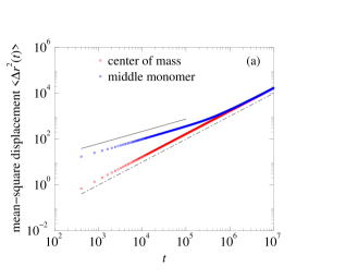
Figure 4: The scaling behaviors for the mean-square displacement $\langle\Delta r^{2}(t)\rangle$: for the center-of-mass (bottom set of points), and for the middle monomer (top set of points). The dot-dashed line corresponds to $\langle\Delta r^{2}(t)\rangle\sim t$ and the solid line corresponds to $\langle\Delta r^{2}(t)\rangle\sim t^{2\nu/(1+2\nu)}$.

which, up to some constant factor, scales with time as $t^{\frac{2\nu}{1+2\nu}}$. Once again, the $t^{\frac{2\nu}{1+2\nu}}$ behavior of the mean-square displacement of the middle monomer will only hold till the lifetime of the lowest mode in the summation of Eq. (17) ($p=2$) scaling as the Rouse time $\tau_{R}\sim N^{1+2\nu}$, after which $\langle\Delta r_{N/2}^{2}\rangle$ has to increase linearly with $t$. Note that Eqs. (16) and (17) confirm the well-known result that by the Rouse time, the middle monomer typically displaces itself by the spatial extent of the polymer $\sim N^{2\nu}$.

In Fig. 4, we confirm the above behavior of the mean-square displacement of the middle monomer and that of the center-of-mass. We have also checked, in support of $X_{00}(t)\sim\delta(t)$, that the probability distribution of the displacement of the center-of-mass of the polymer along all three spatial direction is Gaussian, with the width scaling $\sim\sqrt{t}$ (data not shown).

V.2 Fluctuation dissipation theorem and the anomalous dynamics of the middle monomer

In Secs. II and V we argued that the force on the center-of-mass of the polymer is the average over all the thermal forces on the monomers, leading us to $X_{00}(t)\sim\delta(t)$, which yielded the $\sim t$ behavior of the mean-square displacement of the center-of-mass. This raises the natural question, namely: is it possible to derive the anomalous dynamics of the middle monomer — i.e., the $\langle\Delta r_{N/2}^{2}\rangle\sim t^{\frac{2\nu}{1+2\nu}}$ up to the Rouse time and $\sim t$ thereafter — from the combined forces (internal and external) that act on the middle monomer?

We trace back the formulation of this problem to our recent work on unbiased polymer translocation through a narrow pore in a membrane trans1 . Therein we showed, in the following manner, that the anomalous dynamics of translocation — essentially that of the translocating monomer — can indeed be derived from the forces it experiences. The velocity of translocation $v(t)$ (along the direction perpendicular to the membrane) is related to the force $\phi(t)$ (also acting upon it along the direction perpendicular to the membrane), via the “impedance” memory kernel $\mu(t)$ and “admittance” memory kernel $a(t)$, by

$$\phi(t)=\int_{0}^{t}dt^{\prime}\,\mu(t-t^{\prime})\,v(t^{\prime})+g(t),$$ (18)

and

$$v(t)=\int_{0}^{t}dt^{\prime}\,a(t-t^{\prime})\,\phi(t^{\prime})+h(t).$$ (19)

In Eqs. (18) and (19), $g(t)$ and $h(t)$ are the noise terms satisfying $\langle g(t)\rangle=\langle h(t)\rangle=0$, and the corresponding fluctuation-dissipation theorems $\langle g(t)g(t^{\prime})\rangle=\langle\phi(t)\phi(t^{\prime})\rangle_{v=0}=|\mu(t-t^{\prime})|$ and $\langle h(t)h(t^{\prime})\rangle=\langle v(t)v(t^{\prime})\rangle_{\phi=0}=|a(t-t^{\prime})|$. Moreover, the uniqueness of the relation between $v(t)$ and $\phi(t)$ dictates that their Laplace transforms must satisfy the condition $\mu(z)a(z)=1$. Finally, we characterized the anomalous dynamics of translocation by integrating $\langle v(t)v(t^{\prime})\rangle_{\phi=0}$ twice in time: we obtained the mean-square displacement $\langle s^{2}(t)\rangle$ of the translocating monomer to behave as $t^{\frac{1+\nu}{1+2\nu}}$ until the Rouse time $\tau_{R}$, beyond which $\langle s^{2}(t)\rangle$ linearly with $t$. We showed that the memory kernel scheme works beautifully for translocation out of planar confinements trans2 , translocation by a pulling force at the head of the polymer trans3 (and additional back-pulling voltage trans3a ), field-driven translocation vocks08 , and polymer adsorption adsorb .

It is easy to see in the above analysis that if $\langle\phi(t)\phi(t^{\prime})\rangle_{v=0}=|\mu(t-t^{\prime})|\sim t^{-\alpha}$ for some $\alpha$, then the mean-square displacement of the translocating monomer has to increase as $t^{\alpha}$. We now show that the above scheme established for the anomalous dynamics of polymer translocation also works, with the modification that we now have to deal with vector velocity $\vec{v}(t)$ of the middle monomer and vector force $\vec{f}(t)$ on it, for the anomalous dynamics of the middle monomer of a self-avoiding polymer; namely that we will show that $|\mu(t-t^{\prime})|\sim t^{-\frac{2\nu}{1+2\nu}}$, which would imply $\langle\Delta r_{N/2}^{2}\rangle\sim t^{\frac{2\nu}{1+2\nu}}$. Of course such power-law behavior would only hold till the Rouse time.

In order to do so, we first argue, following Eq. (18), that the impedance memory kernel $\mu(t)$ — that connects the forces on and the velocities of the middle monomer — scales $\sim t^{-\frac{2\nu}{1+2\nu}}$. Consider the thought experiment in which we grab the middle monomer and move it by a small distance $\vec{\delta r}$ and hold it at its new position; this corresponds to $\vec{v}(t)=\vec{\delta r}\,\delta(t)$. In time, the “information” that the middle monomer has moved to a new position at $t=0$ will propagate along the backbone of the polymer, and at time $t$, all the monomers within a backbone distance $n_{t}\sim t^{\frac{1}{1+2\nu}}$ — following the Rouse scaling — will equilibrate to this new situation. These $n_{t}$ equilibrated monomers are however stretched by an amount $\vec{\delta r}$. With the entropic spring constant of $n$ equilibrated monomers scaling $\sim n^{-2\nu}$, the (restoring) force the middle monomer would experience at its new position is given by $\vec{f}(t)\sim n_{t}^{-2\nu}(-\vec{\delta r})\sim t^{-\frac{2\nu}{1+2\nu}}(-\vec{\delta r})$ [force $=$ (spring constant) $\times$ (stretching distance)]. In other words, $\mu(t)\sim t^{-\frac{2\nu}{1+2\nu}}$. The fluctuation-dissipation theorem then dictates that $\langle\vec{f}(t)\cdot\vec{f}(t^{\prime})\rangle|_{\vec{v}=0}=|\mu(t-t^{\prime})|\sim(t-t^{\prime})^{-\frac{2\nu}{1+2\nu}}$ and $\langle\vec{v}(t)\cdot\vec{v}(t^{\prime})\rangle|_{\vec{f}=0}=|a(t-t^{\prime})|\sim(t-t^{\prime})^{-\frac{2(1+\nu)}{1+2\nu}}$. Note once again that these relations only hold till the Rouse time; by the Rouse time the entire polymer is equilibrated to the new position of the middle monomer, and beyond that time the forces on the middle monomer are uncorrelated. Finally, the anomalous dynamics of the middle monomer — $\langle\Delta r_{N/2}^{2}\rangle\sim t^{\frac{2\nu}{1+2\nu}}$ up to the Rouse time and $\sim t$ thereafter — is retrieved by integrating $\langle\vec{v}(t)\cdot\vec{v}(t^{\prime})\rangle_{\vec{f}=0}$ twice in time.

Implementing the above thought experiment into practice and thereby tracking the restoring force on the middle monomer in order to determine $\mu(t)$ is a complicated task. Instead, we focus on the relation $\langle\vec{f}(t)\cdot\vec{f}(t^{\prime})\rangle_{\vec{v}=0}\sim t^{-\frac{2\nu}{1+2\nu}}$. We fix the position of the middle monomer of a self-avoiding polymer (this corresponds to $\vec{v}=0$) and take snapshots of it at equal intervals of time. We then take the snapshot at time $t$, evolve the entire polymer— with its middle monomer free — over $\Delta t=1$ unit of time for a multiple number of times, and obtain the average displacement vector $\vec{u}(t)$ of the middle monomer. Note that $\Delta t=1$ is small enough such that the corresponding Eq. (19) — with $\phi(t)$ and $v(t)$ replaced by $\vec{f}(t)$ and $\vec{v}(t)$ respectively, and $\langle\vec{h}(t)\rangle=0$ — shows that $\vec{u}(t)\propto\vec{f}(t)|_{\vec{v}=0}$. The behavior of $\langle\vec{u}(t)\cdot\vec{u}(t^{\prime})\rangle$ in time then yields the behavior of $\langle\vec{f}(t)\cdot\vec{f}(t^{\prime})\rangle|_{\vec{v}=0}=|\mu(t-t^{\prime})|$. Determined in the above manner, we confirm $|\mu(t)|\sim t^{-\frac{2\nu}{1+2\nu}}\exp(-t/\tau_{R})$ in Fig. 5, with $2\nu/(1+2\nu)\approx 0.54$, from which, as described in the above paragraph, the scaling $\langle\Delta r_{N/2}^{2}\rangle\sim t^{\frac{2\nu}{1+2\nu}}$ can be derived.

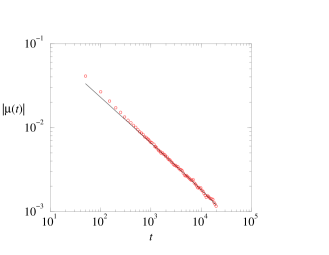
Figure 5: The scaling behavior of $|\mu(t)|$ for $N=400$, determined in the manner described in the text. The solid (black) curve corresponds to $|\mu(t)|=0.275t^{-0.54}\exp(-t/\tau_{R})$, with $\tau_{R}\approx 223801$ for $N=400$, obtained from best-fitting the corresponding data of Fig. 2.

VI Conclusion

To conclude, in this paper we put forward an approximate analytical expression (3) for the mode amplitude correlation functions $X_{pq}(t)$ for long polymers, and corroborate its accuracy using a lattice-based Monte Carlo simulations of self-avoiding flexible polymers in three dimensions in the absence of explicit hydrodynamics. We report that (a) the mode amplitude correlation functions are not exactly statistically independent (we do not expect them to be so anyway); instead, numerically the modes maintain a high degree of statistical independence, and (b) for higher modes ($p,q\gtrsim 6$) there are small deviations from the exponential behavior (3) at long times. Nevertheless, given that $X_{pp}(0)$ is a rapidly decaying function of $p$ as per Eq. (3), the dominant contribution of the modes to quantities of interest for the polymer at long time-scales come from the lower modes. As a result, such quantities can be analytically reconstructed from Eq. (3). We demonstrate this by using Eq. (3) to derive several scaling properties for self-avoiding polymers, such as (i) the real-space end-to-end distance, (ii) the end-to-end vector correlation function, (iii) the correlation function of the small spatial vector connecting two nearby monomers at the middle of the polymer, and (iv) the anomalous dynamics of the middle monomer. Given the content of this paper, we expect that Eq. (3) will provide researchers a way forward for analytical treatment of the properties of self-avoiding polymers.

Importantly, expanding on our recent work on the theory of polymer translocation, we also demonstrate that the anomalous dynamics of the middle monomer can be obtained from the forces it experiences, by the use of the fluctuation-dissipation theorem. Our hope is that in cases where a polymer’s anomalous dynamics exponents are difficult to identify, use of the fluctuation-dissipation theorem will prove to be an indispensably useful tool; first such cases were our recent work on the theory of polymer translocation as well as above.

In experimental situations, the polymer dynamics is often dominated by hydrodynamic interactions. In future work, we therefore intend to extend this study to polymer models with explicit hydrodynamics.

Acknowledgments: D. P. acknowledges ample computer time on the Dutch national supercomputer facility SARA.

References

- (1) M. Doi, Introduction to Polymer Physics, Oxford University Press (Reprinted, 2001).
- (2) M. Doi and S. F. Edwards, The theory of polymer dynamics, Clarendon Press, Oxford (Reprinted, 2001).
- (3) M. Rubinstein, Phys. Rev. Lett. 59, 1946 (1987); T. A. J. Duke, Phys. Rev. Lett. 62, 2877 (1989).
- (4) A. van Heukelum and G. T. Barkema, J. Chem. Phys. 119, 8197 (2003).
- (5) A. van Heukelum et al., Macromol. 36, 6662 (2003).
- (6) J. Klein Wolterink, G.T. Barkema and M.A. Cohen Stuart, Macromolecules 38, 2009 (2005).
- (7) J.K. Wolterink, G.T. Barkema and D. Panja, Phys. Rev. Lett. 96, 208301 (2006).
- (8) D. Panja, G. T. Barkema and R. C. Ball, J. Phys.: Condens. Matter 19, 432202 (2007); D. Panja, G. T. Barkema and R. C. Ball, arxiv:cond-mat/0610671.
- (9) D. Panja, G. T. Barkema and R. C. Ball, J. Phys.: Condens. Matter 20, 075101 (2008).
- (10) D. Panja and G. T. Barkema, Biophys. J. 94, 1630 (2008).
- (11) H. Vocks, D. Panja and G. T. Barkema, J. Phys.: Condens. Matter 21, 375105 (2009).
- (12) H. Vocks et al., J. Phys. Cond. Matt. 20, 095224 (2008).
- (13) D. Panja, G. T. Barkema, A. B. Kolomeisky, J. Phys.: Condens. Matter 21, 242101 (2009).
- (14) J. P. Downey, Macromolecules 27, 2929 (1994).
- (15) T. Kreer et al., Macromolecules 34, 1105 (2001).