Long Delay Times in Reaction Rates Increases Intrinsic Fluctuations

Abstract

In spatially distributed cellular systems, it is often convenient to represent complicated auxiliary pathways and spatial transport by time-delayed reaction rates. Furthermore, many of the reactants appear in low numbers necessitating a probabilistic description. The coupling of delayed rates with stochastic dynamics leads to a probability conservation equation characterizing a non-Markovian process. A systematic approximation is derived that incorporates the effect of delayed rates on the characterization of molecular noise, valid in the limit of long delay time. By way of a simple example, we show that delayed reaction dynamics can only increase intrinsic fluctuations about the steady-state. The method is general enough to accommodate nonlinear transition rates, allowing characterization of fluctuations around a delay-induced limit cycle.

I Introduction

Biochemical circuits underlying many complicated cell functions, disease states, or viral propagation are often modeled by systems of delayed differential equations Mittler et al. (1998); Mahaffy et al. (1998); Lewis (2003); Jensen et al. (2003); Kuske et al. (207); Barrio et al. (2006), where the delay time represents auxiliary reaction pathways or spatial transport. It is well-known that in chemical reaction networks at the cellular level, many of the reactants are present in low copy number and therefore intrinsic noise is simply one of the operating constraints Kerszberg (2004). It is, however, difficult to develop and analyze models that contain both stochastic dynamics and delayed reaction rates.

For systems without delay, a stochastic description typically takes the form of a chemical Master equation that governs the probability distribution $P({\bf n},t)$ of finding the system in state ${\bf n}$ at time $t$ conditioned upon some initial state McQuarrie (1967); Gillespie (1992). The Master equation can rarely be solved exactly, and various methods have been developed to approximate the evolution of $P({\bf n},t)$. Perhaps the most well-known is the Kramers-Moyal expansion, which when truncated after the second term results in a diffusion equation with nonlinear drift and non-constant diffusion, called the Fokker-Planck equation Gillespie (2000); Gardiner (2004). If the deterministic system evolves along a stable trajectory near a stable fixed point, van Kampen van Kampen (1976) has developed an alternate approximation of the Master equation that relies upon a perturbation expansion in some extensive quantity, providing a consistent characterization of the fluctuations in terms of a Fokker-Planck equation with linear drift and constant diffusion from whence the mean and variance are easily computed. (For a more detailed discussion, see van Kampen (1976); Gillespie (2000) and references therein.)

Nevertheless, in many systems the individual reaction events depend upon the past state of the system Kerszberg (2004); Bratsun, D. Volfson, L. S. Tsimring and J. Hasty (2005), and the methods developed to approximate the solution of the Master equation are no longer appropriate. Writing the transition probability of moving from state ${\bf n}^{\prime}$ to state ${\bf n}$ in an interval $dt$ as $W_{{\bf n}^{\prime},{\bf n}}dt$ and the two-point joint probability distribution of finding the system in state ${\bf n}$ at time $t$ and in state ${\bf m}$ at time $t-\tau$ as $P_{2}({\bf n},t;{\bf m},t-\tau)$, the delayed dynamics introduce a convolution term into the probability conservation equation,

$$\frac{\partial P({\bf n},t)}{\partial t}=\sum\limits_{{\bf n}^{\prime}}{W_{{\bf n}^{\prime},{\bf n}}P({\bf n}^{\prime},t)-W_{{\bf n},{\bf n}^{\prime}}P({\bf n},t)}+$$ (1)

$$\sum\limits_{{\bf n}^{\prime}}{\sum\limits_{{\bf m}}{W^{\tau}_{{\bf n}^{\prime},{\bf n}}P_{2}({\bf n}^{\prime},t;{\bf m},t-\tau)-W^{\tau}_{{\bf n},{\bf n}^{\prime}}P_{2}({\bf n},t;{\bf m},t-\tau)}}.$$

Here $W^{\tau}_{{\bf n}^{\prime},{\bf n}}({\bf m})$ depends upon the state at a time $\tau$ in the past: ${\bf m}={\bf n}(t-\tau)$. Eq. 1 is no longer a closed equation for $P({\bf n},t)$ since it now includes the unknown distribution $P_{2}({\bf n},t;{\bf m},t-\tau)$. As a consequence, it no longer describes a Markov process and methods used to treat the standard chemical Master equation require modification.

Many investigations using stochastic simulation algorithms have illustrated the importance of intrinsic noise in systems with delay Lewis (2003); Kerszberg (2004); Barrio et al. (2006), while past analytic work has focused primarily upon approximations of the delayed nonlinear Fokker-Planck equation Guillouzic, I. L Heureux, and A. Longtin (1999); Frank (2005), stochastic delay differential equations Mackey and Nechaeva (1995); Klosek and Kuske (2005); Kuske et al. (207) or exactly-solvable random-walk models Ohira and Milton (1995, 2009). While each provides considerable insight into the interdependent effects of noise and time delay, comparatively little work has been done to connect the underlying discrete probability conservation equation to these continuous approximations. In what follows a perturbation scheme is developed that, under the condition that the delay time exceeds the relaxation time of the deterministic system, allows a general probability conservation equation to be approximated by a delayed linear Fokker-Planck equation, thereby making connection to past studies. Recent work by Bratsun et al. Bratsun, D. Volfson, L. S. Tsimring and J. Hasty (2005) has explored very similar questions, although their method is applicable only to systems with linear reaction rates. The delayed linear noise approximation, which is an extension of van Kampen’s linear noise approximation van Kampen (1976), provides a consistent characterization of intrinsic fluctuations in delayed systems and is sufficient to show that under fairly general conditions delayed reaction events can only increase the magnitude of these fluctuations. A simple example of a birth/death process is used to provide a concrete implementation of the method, and a nonlinear predator-prey model illustrates characterization of fluctuations along a delay-induced limit cycle.

II Mathematical methods

A stochastic model of a network of chemical reactions governs the probability distribution $P({\bf n},t)$ of finding the system in state ${\bf n}$ at time $t$, with dynamics given in terms of the stoichiometric change resulting from the completion of each reaction and the propensity of occurrence for each reaction event, recorded, respectively, in the stoichiometry matrix ${\bf S}$ and the propensity vector $\tilde{\bm{\nu}}$ Gillespie (1977); Elf and M. Ehrenberg (2003). Consider a system with $N$ reactants that can combine through one of $R$ reactions. To facilitate the inclusion of delayed kinetics into the formalism, we separate the $R$ reactions into two groups: those with rates $\left\{{\tilde{\nu}_{j}\left({\mathbf{n}}\right)}\right\}_{j=1}^{R_{c}}$ depending upon the current state of the system and those with rates $\left\{\varepsilon{\tilde{\nu}_{j}\left({{\mathbf{m}},{\mathbf{n}}}\right)}\right\}_{j=R_{c}+1}^{R}$ depending upon the past state of the system ${\mathbf{m}}={\mathbf{n}}\left({t-\tau}\right)$, where $\tau$ is the delay time. The parameter $\varepsilon$ measures the delayed feedback strength; throughout, we shall assume that the feedback is weak, and explicitly retain leading-order terms in $\varepsilon$.

To keep the notation compact, we introduce the step-operator ${\bf E}_{i}^{-S_{ij}}$ that acts to increment the variable $n_{i}$ by an integer $-S_{ij}$: ${\bf E}_{i}^{-S_{ij}}f(n_{i})=f(n_{i}-S_{ij})$. Denoting the system volume by $V$, Eq. 1 takes the form van Kampen (1992); Elf and M. Ehrenberg (2003); Bratsun, D. Volfson, L. S. Tsimring and J. Hasty (2005),

$$\frac{{\partial P}}{{\partial t}}=V\mathop{\sum\limits_{j=1}^{R_{c}}{\left[{\left({\prod\limits_{i=1}^{N}{{\mathbf{E}}_{i}^{-S_{ij}}}}\right)-1}\right]\tilde{\nu}_{j}\left({\mathbf{n}}\right)P\left({{\mathbf{n}},t}\right)}}\limits_{{\text{current - state dynamics}}}+V\mathop{\sum\limits_{j=R_{c}+1}^{R}{\left[{\left({\prod\limits_{i=1}^{N}{{\mathbf{E}}_{i}^{-S_{ij}}}}\right)-1}\right]\sum\limits_{\mathbf{m}}{\varepsilon\tilde{\nu}_{j}\left({{\mathbf{m}},{\mathbf{n}}}\right)\Theta\left({\left\{{n_{i}}\right\}}\right)P_{2}\left({{\mathbf{n}},t;{\mathbf{m}},t-\tau}\right)}}}\limits_{{\text{delayed - state dynamics}}},$$ (2)

where $\Theta\left({\left\{{n_{i}}\right\}}\right)$ is the Heaviside-step function that ensures no delayed reaction occurs if completion results in the unphysical end-state $n_{i}<0$ for any elements of ${\bf n}$. Throughout, only non-consuming reactions are considered Barrio et al. (2006); Cai (2007), i.e. reactants of an unfinished reaction are allowed to participate in new reactions.

The solution of the full distribution $P\left({{\mathbf{n}},t}\right)$ is not possible in general, therefore we seek an approximate solution. To that end, we make the ansatz that the number of reactant molecules is large enough that the discrete molecule numbers $n_{i}$ can be represented by the continuous deterministic concentrations $x_{i}$ and some continuous fluctuations $\alpha_{i}$ that scale as the square-root of the number of molecules van Kampen (1976),

$$n_{i}=Vx_{i}+\sqrt{V}\alpha_{i}\quad\mbox{and}\quad m_{i}=Vx_{i}^{\tau}+\sqrt{V}\beta_{i},$$ (3)

where $V$ is the system volume and $x_{i}^{\tau}\equiv x_{i}\left({t-\tau}\right)$. Using the auxiliary variable $\beta_{i}$, the delayed fluctuations are written as $\beta_{i}\left({t-\tau}\right)=\alpha_{i}\left({t-\tau}\right)$ to emphasize the approximation made below; specifically, that the delay time is sufficiently large that $\alpha_{i}$ and $\beta_{i}$ can be treated as independent random functions. As we show below (Eq. 18), that assumption is consistent with the requirement that the delay time is much larger than the characteristic relaxation time of the deterministic equations and that the delayed feedback is weak ($\varepsilon\ll 1$). In the expansion below, $1/V$ is assumed small, although since $x_{i}$ is held fixed, (equivalently, one assumes that $n_{i}$ is large). The resulting approximation will be called the delayed linear noise approximation.

Invoking the linear noise approximation by Taylor-expanding the microscopic transition rates about the macroscopic trajectory ${\mathbf{x}}\left(t\right)$ in powers of $\sqrt{V}$ van Kampen (1976); Elf and M. Ehrenberg (2003), we have

$$\tilde{\nu}_{j}\left({{\mathbf{m}},{\mathbf{n}},V}\right)\approx\nu_{j}\left({{\mathbf{x}}^{\tau},{\mathbf{x}}}\right)+\frac{1}{\sqrt{V}}\sum\limits_{i=1}^{N}{\left[{\frac{{\partial\nu_{j}}}{{\partial x_{i}}}\alpha_{i}+\frac{{\partial\nu_{j}}}{{\partial x_{i}^{\tau}}}\beta_{i}}\right]},$$

with an analogous expression for $\tilde{\nu}_{j}\left({{\mathbf{n}},V}\right)$. The rates $\nu_{j}$ correspond to the deterministic reaction rates (see Elf and M. Ehrenberg (2003) for a discussion of the difference between $\tilde{\bm{\nu}}$ and ${\bm{\nu}}$). The discrete step-operator $\mathbf{E}$ is likewise expressed as a Taylor series in $\sqrt{V}^{-1}$ van Kampen (1976); Elf and M. Ehrenberg (2003),

$$\prod\limits_{i=1}^{N}{{\mathbf{E}}_{i}^{-S_{ij}}}=1-\frac{1}{{\sqrt{V}}}\sum\limits_{i=1}^{N}{S_{ij}\partial_{i}}+\frac{1}{{2V}}\sum\limits_{i,k=1}^{N}{S_{ij}S_{kj}\partial_{i}\partial_{k}},$$

where $\partial_{i}={\partial\mathord{\left/{\vphantom{\partial{\partial\alpha_{i}}}}\right.\kern-1.2pt}{\partial\alpha_{i}}}$. The one-point $P\left({{\mathbf{n}},t}\right)$ and two-point joint probability $P_{2}\left({{\mathbf{n}},t;{\mathbf{m}},t-\tau}\right)$ can be written in terms of the single distribution and joint distribution of the fluctuations about the macroscopic trajectory, $\Pi\left({\bm{\alpha},t}\right)$ and $\Pi_{2}\left({\bm{\alpha},t;\bm{\beta},t-\tau}\right)$, respectively, via the linear change of variables suggested by Eq. 3,

$$P\left({{\mathbf{n}},t}\right)=V^{-N/2}\Pi\left({\bm{\alpha},t}\right),$$ (4)

$$P_{2}\left({{\mathbf{n}},t;{\mathbf{m}},t-\tau}\right)=V^{-N}\Pi_{2}\left({\bm{\alpha},t;\bm{\beta},t-\tau}\right),$$ (5)

where ${\bm{\alpha}}$ and ${\bm{\beta}}$ are centered upon ${\mathbf{x}}\left(t\right)$ and ${\mathbf{x}}\left({t-\tau}\right)$, respectively, and the factor involving $V$ comes from the normalization of $\Pi$,

$$\int_{-\infty}^{\infty}P\left({{\mathbf{n}},t}\right)d{\mathbf{n}}=V^{-N/2}\int_{-\infty}^{\infty}\Pi\left({\bm{\alpha},t}\right)d{\bm{\alpha}}=1.$$ (6)

The decoupling of the deterministic component ${\bm{x}}$ from the stochastic component ${\bm{\alpha}}$, with a $1/\sqrt{V}$ scaling of the fluctuations implied by the ansatz Eq. 3, is the most fundamental step in the approximation. That assumption leads directly to the normalization above, and allows subsequent terms in the perturbation expansion to be ordered in terms of powers of $1/\sqrt{V}$ van Kampen (1976).

For long delay time $\tau$, and small delayed-feedback strength $\varepsilon$, the fluctuations at time $t$ are approximately independent of the fluctuations at time $t-\tau$, allowing the joint-distribution to be factored as,

$$\Pi_{2}\left({\bm{\alpha},t;\bm{\beta},T}\right)\approx\Pi\left({\bm{\alpha},t}\right)\times\Pi\left({\bm{\beta},T}\right)+\varepsilon h({\bm{\alpha}},{\bm{\beta}})$$ (7)

$$\quad T\leq t-\tau,$$

where $h({\bm{\alpha}},{\bm{\beta}})$ must obey the consistency condition,

$$\int h({\bm{\alpha}},{\bm{\beta}})d{\bm{\alpha}}=\int h({\bm{\alpha}},{\bm{\beta}})d{\bm{\beta}}=0.$$

Notice the factoring of the fluctuations $\Pi_{2}$ is not equivalent with assuming independence in the full state, $P({\bf n},t;{\bf m},\tau)=P({\bf n},t)\times P({\bf m},\tau)$ (as is done in Bratsun, D. Volfson, L. S. Tsimring and J. Hasty (2005)). Independence of the full state is inconsistent with the deterministic rate equations,

$$\frac{{d{\mathbf{x}}}}{{dt}}={\mathbf{S}}\cdot\bm{\nu}={\mathbf{f}}\left({{\mathbf{x}}^{\tau},{\mathbf{x}}}\right),$$ (8)

where, in the limit of large ${\bf n}$, the present state is completely determined by the past-states (except, perhaps, at steady-state). Moreover, independence of the full state implies that higher-order correlations, including the autocorrelation function $K(t-s)$, vanish for $|t-s|>\tau$. We show below (Eq. 18) that this is not the case.

In the limit $1/V\to 0\;(n_{i}\to\infty)$, the Heaviside step function is $\Theta\left({\left\{{n_{i}}\right\}}\right)=1$, and with the factored joint distribution, Eq. 7, the sum over ${\bf m}$ is replaced by the integral over ${\bm{\beta}}$,

$$\int\limits_{-\infty}^{\infty}{\left\{{\nu_{j}+\frac{1}{\sqrt{V}}\sum\limits_{i=1}^{N}{\left[{\frac{{\partial\nu_{j}}}{{\partial x_{i}}}\alpha_{i}+\frac{{\partial\nu_{j}}}{{\partial x_{i}^{\tau}}}\beta_{i}}\right]}}\right\}V^{-N}\Pi\left({\bm{\alpha},t}\right)\Pi\left({\bm{\beta},t-\tau}\right)d{\bm{\beta}}}=\left\{{\nu_{j}+\frac{1}{\sqrt{V}}\sum\limits_{i=1}^{N}{\left[{\frac{{\partial\nu_{j}}}{{\partial x_{i}}}\alpha_{i}+\frac{{\partial\nu_{j}}}{{\partial x_{i}^{\tau}}}\left\langle{\beta_{i}}\right\rangle}\right]}}\right\}V^{-\frac{N}{2}}\Pi\left({\bm{\alpha},t}\right).$$

Here, the first two terms on the right-hand side follow from the normalization condition on $\Pi(\bm{\beta},t-\tau)$, Eq. 6, and the third from,

$$V^{-N/2}\int_{-\infty}^{\infty}\beta_{i}\Pi(\bm{\beta},t-\tau)d\bm{\beta}=\langle\beta_{i}\rangle.$$

Substituting the expanded terms in Eq. 2, using the chain-rule to write the partial derivatives of $P({\bf n},t)$ in terms of $\Pi$ and ${\bm{\alpha}}$ van Kampen (1976), and collecting in powers of $\sqrt{V}$, the zero’th order term is simply the deterministic delayed reaction rate equations, Eq. 8. At ${\sqrt{V}}^{-1}$, we obtain the equation characterizing the probability distribution of the fluctuations ${\bm{\alpha}}(t)$,

$$\begin{split}\frac{{\partial\Pi}}{{\partial t}}=\sum\limits_{i,j}{-\Gamma_{ij}\partial_{i}\left({\alpha_{j}\Pi}\right)+\frac{D_{ij}}{2}\partial_{ij}\Pi-\varepsilon\Gamma_{ij}^{\tau}\left\langle{\beta_{j}}\right\rangle\partial_{i}\Pi},\end{split}$$ (9)

where,

$$\Gamma_{ij}=\frac{{\partial[{\bm{S}}\cdot{\bm{\nu}}]_{i}}}{{\partial x_{j}}},\;\varepsilon\Gamma_{ij}^{\tau}=\frac{{\partial[{\bm{S}}\cdot{\bm{\nu}}]_{i}}}{{\partial x_{j}^{\tau}}},\;{\bm{D}}={\mathbf{S}}\cdot\mbox{diag}\left[\bm{\nu}\right]\cdot{\mathbf{S}}^{T}.$$

Eq. 9 is a closed diffusion equation for $\Pi({\bm{\alpha}},t)$ with coefficients that are linear in the fluctuation variables ${\bm{\alpha}}$. The matrix ${\bm{D}}$ represents the diffusive effects of the fluctuations, while the matrices ${\bm{\Gamma}}$ and ${\bm{\Gamma}^{\tau}}$ represent the restorative drift in the system Scott, B. Ingalls and M. Kaern (2006); van Kampen (1992). Eq. 9 is not quite a Fokker-Planck equation since it contains the delayed average $\langle\beta_{j}\rangle\equiv\langle\alpha_{j}(t-\tau)\rangle$ in the drift coefficient. Nevertheless, the initial conditions can be chosen so that the last term in Eq. 9 vanishes, as we now show. Multiplying $\frac{{\partial\Pi}}{{\partial t}}$ by $\alpha_{i}$ and integrating yields the evolution equation for the mean,

$$\frac{{d\left\langle{\bm{\alpha}\left(t\right)}\right\rangle}}{{dt}}={\bm{\Gamma}}\cdot\left\langle{\bm{\alpha}\left(t\right)}\right\rangle+\varepsilon{\bm{\Gamma}}^{\tau}\cdot\left\langle{\bm{\alpha}\left({t-\tau}\right)}\right\rangle.$$ (10)

The initial average $\langle\bm{\alpha}(t)\rangle$ can always be absorbed into the initial conditions on ${\mathbf{x}}\left(t\right)$ so that $\left\langle{\bm{\alpha}\left(t\right)}\right\rangle=0$ for $t\leqslant 0$, thereby ensuring that $\left\langle{\bm{\alpha}\left(t\right)}\right\rangle=0$ for all time. Without loss of generality, then, we write Eq. 9 as the Fokker-Planck equation with coefficients linear in $\bm{\alpha}$,

$$\frac{{\partial\Pi}}{{\partial t}}=-\sum\limits_{i,j}{\Gamma_{ij}\partial_{i}\left({\alpha_{j}\Pi}\right)}+\frac{1}{2}\sum\limits_{i,j}{D_{ij}\partial_{i}\partial_{j}\Pi}.$$ (11)

It is important to note that although the fluctuations at time $t$ are independent of fluctuations in the past, they are conditioned by the macroscopic solution ${\mathbf{x}}\left({t}\right)$ (and ${\mathbf{x}}\left({t-\tau}\right)$) through the coefficient matrices ${\bm{\Gamma}}$ and ${\bf D}$.

A consequence of Eq. 11 is that, to $O\left({V^{-1}}\right)$ , the fluctuations are Gaussian distributed with covariance $\Xi_{ij}=\left\langle{\alpha_{i}\alpha_{j}}\right\rangle-\left\langle{\alpha_{i}}\right\rangle\left\langle{\alpha_{j}}\right\rangle=\left\langle{\alpha_{i}\alpha_{j}}\right\rangle$. Multiplying Eq. 11 by $\alpha_{i}\alpha_{j}$ and integrating over all ${\bm{\alpha}}$ yields a dynamic equation governing ${\bm{\Xi}}$ (van Kampen, 1992, p. 211),

$$\frac{d{\bm{\Xi}}}{dt}={\bm{\Gamma}}\cdot{\bm{\Xi}}+{\bm{\Xi}}\cdot{\bm{\Gamma}}^{\dagger}+{\bf D},$$ (12)

(where ${\bm{\Gamma}}^{\dagger}$ is the matrix transpose of ${\bm{\Gamma}}$; not to be confused with ${\bm{\Gamma}}^{\tau}$). At steady-state, the coefficient matrices ${\bm{\Gamma}}$ and ${\bf D}$ (and therefore ${\bm{\Xi}}$) will be constant, satisfying the fluctuation-dissipation relation,

$${\bm{\Gamma}}\cdot{\bm{\Xi}}+{\bm{\Xi}}\cdot{\bm{\Gamma}}^{\dagger}+{\bf D}=0.$$ (13)

The diffusion matrix ${\bf D}$ is symmetric and positive semi-definite by construction, so that a steady-state probability distribution is only possible if the drift term ${\bm{\Gamma}}$ balances the diffusion ${\bf D}$. With long-delay in the reaction kinetics, the restorative influence of ${\bm{\Gamma}}^{\tau}$ no longer appears in the equation governing the fluctuations (Eq. 11), so that although the delayed dynamics increase the magnitude of the diffusion matrix ${\bm{D}}$, the dissipation due to ${\bm{\Gamma}}^{\tau}$ is lost. Therefore, in the limit of long delay time, delayed dynamics can only serve to increase the magnitude of intrinsic fluctuations.

III Steady-state autocorrelation function and spectrum

The fluctuation-dissipation relation, Eq. 13, and the evolution equation for the mean, Eq. 10, together provide an expression for the time-autocorrelation matrix for the fluctuations about the steady-state, ${\bf K}(t)=\langle{\bm{\alpha}}(t)\cdot{\bm{\alpha}}^{T}(0)\rangle$. The steady-state autocorrelation function ${\bf K}(t)$ is, by definition,

$${\mathbf{K}}\left(t\right)=\iint{{\bm{\alpha}}^{\prime}\left(t\right)\cdot{\bm{\alpha}}^{T}\left(0\right)\Pi_{2}\left({{\bm{\alpha}}^{\prime},t;{\bm{\alpha}},0}\right)d{\bm{\alpha}}^{\prime}d{\bm{\alpha}}}.$$

Re-writing in terms of the conditional probability,

$${\mathbf{K}}\left(t\right)=\iint{{\bm{\alpha}}^{\prime}\left(t\right)\cdot{\bm{\alpha}}^{T}\left(0\right)\Pi\left({{\bm{\alpha}}^{\prime},t|{\bm{\alpha}},0}\right)\Pi\left({{\bm{\alpha}},0}\right)d{\bm{\alpha}}^{\prime}d{\bm{\alpha}}}$$

$${\mathbf{K}}\left(t\right)=\iint{\left\langle{{\bm{\alpha}}\left(t\right)}\right\rangle_{{\bm{\alpha}}\left(0\right)}\cdot{\bm{\alpha}}^{T}\left(0\right)\Pi\left({{\bm{\alpha}},0}\right)d{\bm{\alpha}}},$$ (14)

where ${\left\langle{{\bm{\alpha}}\left(t\right)}\right\rangle_{{\bm{\alpha}}\left(0\right)}}$ is the solution of Eq. 10 with initial condition ${\bm{\alpha}}(0)$, and $\Pi$ is the equilibrium distribution of ${\bm{\alpha}}(0)$ Bratsun, D. Volfson, L. S. Tsimring and J. Hasty (2005); van Kampen (1965). Eq. 7 requires that the conditional probability density $\Pi({\bm{\alpha}}^{\prime},t|{\bm{\alpha}},0)$ be written as a perturbation expansion in $\varepsilon$,

$$\Pi({\bm{\alpha}}^{\prime},t|{\bm{\alpha}},0)=\Pi^{0}({\bm{\alpha}}^{\prime},t|{\bm{\alpha}},0)+\varepsilon\Pi^{1}({\bm{\alpha}}^{\prime},t|{\bm{\alpha}},0)+O(\varepsilon^{2}).$$ (15)

Consequently, in the conditional average ${\left\langle{{\bm{\alpha}}\left(t\right)}\right\rangle_{{\bm{\alpha}}\left(0\right)}}$, only terms to first-order in $\varepsilon$ are retained.

The conditional average ${\left\langle{{\bm{\alpha}}\left(t\right)}\right\rangle_{{\bm{\alpha}}\left(0\right)}}$ is obtained from Eq. 10, which is easily solved via Laplace transform. The equilibrium correlation function is an even function of time-difference alone, equivalent to boundary condition $\left\langle{{\bm{\alpha}}\left(t\right)}\right\rangle=0$ for $t<0$, leading to the formal solution

$$\left\langle{\hat{\bm{\alpha}}\left(s\right)}\right\rangle_{\alpha\left(0\right)}=\left[{s{\mathbf{I}}-{\bf\Gamma}-\varepsilon e^{-s\tau}{\bf\Gamma}^{\tau}}\right]^{-1}\cdot\left\langle{{\bm{\alpha}}\left(0\right)}\right\rangle.$$ (16)

The derivation of Eq. 11 assumes $\varepsilon\to 0$, so to remain consistent, we retain only leading-order terms in $\varepsilon$ in the Laplace transform of the mean,

$$\left\langle{\hat{\bm{\alpha}}\left(s\right)}\right\rangle=\left[{s{\mathbf{I}}-{\bf\Gamma}}\right]^{-1}\cdot\left\langle{{\bm{\alpha}}\left(0\right)}\right\rangle$$

$$+\varepsilon e^{-s\tau}\left[{s{\mathbf{I}}-{\bf\Gamma}}\right]^{-1}\cdot{\bf\Gamma}^{\tau}\cdot\left[{s{\mathbf{I}}-{\bf\Gamma}}\right]^{-1}\cdot\left\langle{{\bm{\alpha}}\left(0\right)}\right\rangle.$$ (17)

With substitution into Eq. 14, using the fluctuation-dissipation relation, Eq. 13, the autocorrelation function is

$${\bf K}(t)=\exp\left[{{\bf\Gamma}t}\right]\cdot{\bm{\Xi}}_{s}$$ (18)

$$+\varepsilon\Theta(t-\tau)\mathfrak{L}_{t-\tau}^{-1}\left\{{\left[{s{\mathbf{I}}-{\bf\Gamma}}\right]^{-1}\cdot{\bf\Gamma}^{\tau}\cdot\left[{s{\mathbf{I}}-{\bf\Gamma}}\right]^{-1}}\right\}\cdot{\bm{\Xi}}_{s},$$

where $\Theta(t-\tau)$ is the Heaviside step function, and $\mathfrak{L}_{t-\tau}^{-1}$ is the time-shifted inverse Laplace transform. The first term produces an exponential drop from $t=0$, while the second term produces an anti-correlated second peak slightly beyond $t=\tau$; higher-order terms in $\varepsilon$ produce alternating correlated/anti-correlated peaks of magnitude $O(\varepsilon^{n})$ for the $n^{th}$ peak.

The fluctuation spectrum follows immediately from the autocorrelation function. We denote the $\varepsilon$-correction to the autocorrelation function $\hat{\bm{K}}_{corr}(s)$,

$$\hat{\bm{K}}_{corr}(s)=e^{-s\tau}\left[{s{\mathbf{I}}-{\bm{\Gamma}}}\right]^{-1}\cdot{\bm{\Gamma}}^{\tau}\cdot\left[{s{\mathbf{I}}-{\bm{\Gamma}}}\right]^{-1},$$ (19)

then the spectrum $S(\omega)$ is Gardiner (2004),

$$S(\omega)=\int_{0}^{\infty}e^{-i\omega t}{\bf K}(t)dt+\int_{-\infty}^{0}e^{i\omega t}{\bf K}^{\dagger}(-t)dt$$

$$=\left[{-i\omega{\mathbf{I}}+{\bm{\Gamma}}}\right]^{-1}\cdot{\mathbf{D}}\cdot\left[{i\omega{\mathbf{I}}+{\bm{\Gamma}}^{\dagger}}\right]^{-1}$$

$$+\varepsilon\left\{{{\mathbf{K}}_{corr}\left({i\omega}\right)\cdot\Xi_{s}+\Xi_{s}\cdot{\mathbf{K}}_{corr}^{\dagger}\left({-i\omega}\right)}\right\},$$ (20)

where ${\bf D}$ is the diffusion matrix introduced in Eq. 9 evaluated at the steady-state.

Figure 1: Fano factor as a function of delay time. The $\tau=0$ (dotted) and $\tau\to\infty$ (solid) approximations to the Fano factor, $\mbox{var}[x]/\langle x\rangle$ (Eq. 28), provide lower and upper bounds on the estimate of intrinsic noise over the range of delay times, as compared to stochastic simulation data generated from the model shown in Eq. 24 (filled circles). The delayed linear noise approximation adequately characterizes the fluctuations even when the delay time is of the order of the other time scales in the problem (i.e. $\tau\delta\approx 1$). Here, the deterministic reaction rates are $\gamma=100$, $\delta=4$, $\varepsilon=1/4$, with $V=1$. Simulation data is from an ensemble of $10^{5}$ members using the delayed Gillespie algorithm Cai (2007).

IV Linear example - Delayed protein degradation

To provide some context for the formal derivation above, consider a simple birth/death model with delayed degradation Bratsun, D. Volfson, L. S. Tsimring and J. Hasty (2005). The total number of species $X$ evolves via the following three reactions,

$$\begin{array}[]{*{20}c}{\mbox{constant synthesis:}}&{X\overset{\nu_{1}}{\rightarrow}X+1;}&{\nu_{1}=\gamma},\\ {\mbox{linear degradation:}}&{X\overset{\nu_{2}}{\rightarrow}X-1;}&{\nu_{2}=\delta\cdot x},\\ {\mbox{delayed degradation:}}&{X\overset{\nu_{3}}{\Rightarrow}X-1;}&{\nu_{3}=\varepsilon\delta\cdot x^{\tau}}.\\ \end{array}$$ (24)

The reaction rate vector (in units of concentration/time) is given by ${\bm{\nu}}=[{\gamma,\delta\cdot x,\varepsilon\delta\cdot x^{\tau}}]$ and the stoichiometry matrix is ${\bf S}=[1,-1,-1]$. The deterministic reaction rate equation for the concentration $x(t)$ is then governed by the delayed differential equation, $\dot{x}={\bf S}\cdot{\bm{\nu}}=\gamma-\delta\cdot x-\varepsilon\delta\cdot x^{\tau}$. The auxiliary coefficient matrices in Eq. 11 are the scalars ${\bm{\Gamma}}=-\delta$ and ${\bf D}=\gamma+\delta\cdot x+\varepsilon\delta\cdot x^{\tau}$. For the sake of simplicity, we consider the fluctuations about the steady-state $x_{s}$, where $x_{s}=\gamma/\delta(1+\varepsilon)$. From Eq. 13, the variance of the fluctuations about $x_{s}$ is, (using Eq. 3),

$$\langle{\left({\frac{X}{V}}\right)^{2}}\rangle-\langle x_{s}\rangle^{2}=\frac{\langle\alpha^{2}\rangle}{V}=\frac{{\Xi}}{V}=\frac{1}{V}\frac{\gamma}{\delta}.$$

A useful measure of the relative magnitude of the fluctuations is the fractional deviation $\eta_{\tau}^{2}$,

$$\eta_{\tau\to\infty}^{2}=\frac{\Xi}{V\cdot x_{s}^{2}}=\frac{1}{N_{s}}(1+\varepsilon),$$ (25)

where here $N_{s}=V\cdot x_{s}$ is the number of molecules in the steady-state. Without delay, this simple example describes a Poisson process, and for a Poisson process the Fano factor $F=\eta^{2}N_{s}=\Xi/x_{s}=1$. From Eq. 25,

$$F=\left\{{\begin{array}[]{*{20}c}{1,}&{\tau\to 0}\\ {1+\varepsilon,}&{\tau\to\infty.}\\ \end{array}}\right.$$ (28)

The Fano factor is a particularly convenient statistic to contrast the ordinary and delayed linear noise approximations, as well as illustrating the delay time necessary for the present approximation to hold. Figure 1 shows the Fano factor $F$ estimated from stochastic simulation Gillespie (1977); Cai (2007) with $\gamma=100$, $\delta=4$ and $\varepsilon=0.25$, as compared with the long delay time (solid) and short delay time (dotted) estimates. Notice the cross-over occurs for $\tau\approx\delta^{-1}$, that is for delay time comparable to the natural time scale of the undelayed kinetics.

The autocorrelation function is given by Eq. 18,

$$K(t)=e^{-\delta t}\left\{{1-\varepsilon\Theta\left({t-\tau}\right)\delta e^{\delta\tau}\left({t-\tau}\right)}\right\}\frac{{\gamma}}{{\delta}}.$$ (29)

This expression coincides with the result of Bratsun et al. Bratsun, D. Volfson, L. S. Tsimring and J. Hasty (2005) to $O(\varepsilon)$, and as they demonstrate, $K(t)$ very faithfully reproduces the autocorrelation from simulation data. Furthermore, the autocorrelation can be used to identify ‘quasi-cyles’ where regular oscillations emerge from deterministically stable systems Klosek and Kuske (2005); McKane and Newman (2005); Scott et al. (2007); Boland et al. (2008).

The delayed-degradation model is used as a transparent illustration of the method, but the same results can be obtained by other methods (for example, via moment-generating functions Bratsun, D. Volfson, L. S. Tsimring and J. Hasty (2005)). In contrast, the model in the next section contains more realistic, nonlinear transition rates, and consequently cannot be treated by existing methods. Yet nonlinear rates abound in physical application and exhibit rich dynamics, as the following example demonstrates.

V Nonlinear example - Predator-Prey Dynamics

The methodology outlined in Section II makes no assumptions about the nonlinearity of the transition probabilities in the stochastic model, opening up the possibility to study the dynamics of delayed nonlinear systems. As an example capable of exhibiting asymptotic stability and limit cycle behavior, consider the predator-prey model with delayed predator birth,

$$\frac{dP}{dt}=a\cdot P(t)-\frac{a}{K}\cdot P(t)^{2}-b\cdot P(t)Z(t),$$

$$\frac{dZ}{dt}=c\cdot P(t-\tau)Z(t-\tau)-d\cdot Z(t),$$

where $P(t)$ is the density of prey, $Z(t)$ is the density of predators and $K$ is the carrying capacity of the environment. Here, $\tau$ is the delay time associated with gestation before the birth of predators. Assuming each birth event produces a litter of $1$, the reaction network, in volume $V$, takes the form,

$$\begin{array}[]{*{20}c}P&{\overset{\nu_{1}}{\rightarrow}}&{P+1;}&{}\hfil&{\nu_{1}=a\cdot\frac{{n_{P}}}{V}}\\ P&{\overset{\nu_{2}}{\rightarrow}}&{P-1;}&{}\hfil&{\nu_{2}=\frac{a}{K}\cdot\frac{{n_{P}}}{V}\cdot\frac{{n_{P}-1}}{V}}\\ P&{\overset{\nu_{3}}{\rightarrow}}&{P-1;}&{}\hfil&{\nu_{3}=b\cdot\frac{{n_{P}}}{V}\cdot\frac{{n_{Z}}}{V}}\\ Z&{\overset{\nu_{4}}{\rightarrow}}&{Z-1;}&{}\hfil&{\nu_{4}=d\cdot\frac{{n_{Z}}}{V}}\\ Z&\overset{\nu_{5}}{\Rightarrow}&{Z+1;}&{}\hfil&{\nu_{5}=c\cdot\frac{{n_{P}\left({t-\tau}\right)}}{V}\cdot\frac{{n_{Z}\left({t-\tau}\right)}}{V},}\\ \end{array}$$ (35)

where $n_{P}/V=P(t)$ and $n_{Z}/V=Z(t)$.

With a suitable nondimensionalization,

$$t_{0}=1/a,\;\;P_{0}=K,\;\;Z_{0}=a/b,\;\;\epsilon=c\cdot K/a,\;\mbox{and}\;\delta=d/a,$$

the deterministic model equations reduce to,

$$\frac{dP}{dt}=P(t)-P(t)^{2}-P(t)Z(t),$$

$$\frac{dZ}{dt}=\varepsilon\cdot P(t-\tau)Z(t-\tau)-\delta\cdot Z(t),$$ (36)

where $\tau$ has been likewise nondimensionalized by $1/a$. The equilibrium point corresponding to coexistence of the populations is $(P,Z)=(\frac{\delta}{\varepsilon},1-\frac{\delta}{\varepsilon})$, leading to a necessary condition for stable coexistence, with and without delay, that $\delta<\varepsilon$.

It is well-known that delayed rates can have a destabilizing effect on population dynamics May (1973), and in fact can generate limit-cycles in otherwise stable models Tiana et al. (2002); Krishna et al. (2006); Barrio et al. (2006). To illustrate the approximation method and the destabilizing effects of delay, we consider two values for the delay time, $\tau=0$ and $\tau=30$, in two parameter regimes – the first chosen so that the equilibrium remains asymptotically stable for both values of the delay time, the second chosen so that a limit-cycle appears for large delay $\tau$.

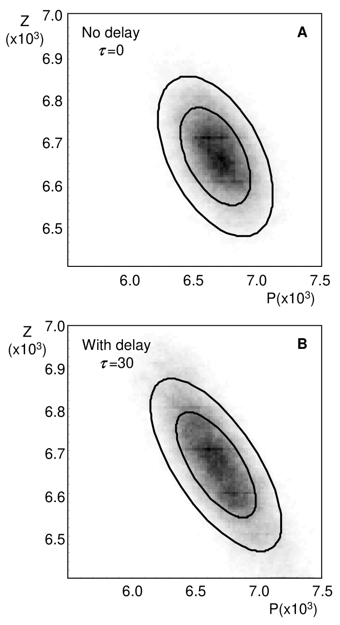
Figure 2: Steady-state fluctuations in a nonlinear model ($\varepsilon=0.15,\delta=0.05$). A. Density plot of the equilibrium fluctuations from stochastic simulation ($10^{6}$ realizations). Solid curves correspond to the first- and second-standard deviation ellipse computed by an ordinary application of the linear noise approximation van Kampen (1976). B. Same model parameters as in panel A, but with delayed predator birth ($\tau=30$). The solid curves correspond to the first- and second-standard deviation ellipse computed by the delayed linear noise approximation.

V.1 Asymptotically stable

For ($\varepsilon=0.15,\delta=0.05$), the system remains asymptotically stable in both limits, $\tau=0$ (Figure 2A) and $\tau=30$ (Figure 2B). From Eq. 13, long delay time reduces the stability imparted to the system through $\Gamma$. As a consequence, the variance of the fluctuations is expected to increase with increasing delay time $\tau$. This increase is evident in the stationary probability distribution of the fluctuations derived from stochastic simulation (Figure 2). The ellipses shown in the figure correspond to the first- and second-standard deviations of the steady-state Gaussian distribution predicted by the approximation, while the density plot represents extensive stochastic simulation data generated using Gillespie’s algorithm Gillespie (1977); Cai (2007).

The most striking consequence of the delay on the intrinsic fluctuations is the increased magnitude of the cross-correlation between $P$ and $Z$. As $\tau\to\infty$, the delayed rate $c\cdot P(t-\tau)Z(t-\tau)$ no longer offers compensation to the predation event with rate $-b\cdot P(t)Z(t)$, resulting in the increased cross-correlation. This is an example of the nontrivial effect of delayed dynamics on intrinsic fluctuations, even though the equilibrium point is stable. In situations where the delay affects not only the fluctuations, but the underlying stability itself (as is the case for delay induced limit cycles), the analysis becomes more complicated.

Figure 3: Fluctuations around a delay-induced limit cycle ($\varepsilon=0.25,\delta=0.05$). A. Envelope of the standard-deviation of the fluctuations transverse to the limit cycle, as computed by Eq.37 using the delayed linear noise approximation. B. Stochastic simulation of the system along the limit cycle.

V.2 Limit cycle

For ($\varepsilon=0.25,\delta=0.05$), the system is asymptotically stable for $\tau=0$, but a limit-cycle appears for $\tau=30$. By separating the fluctuations tangent to the limit cycle from those transverse Tomita, T. Ohta and H. Tomita (1974); Ali and M. Menzinger (1999); Scott, B. Ingalls and M. Kaern (2006); Boland et al. (2008), the delayed linear noise approximation is easily extended to a system exhibiting a limit-cycle.

Briefly, a moving coordinate frame is introduced using as a basis the unit vectors tangent (${\bm{\hat{}}s}$) and normal (${\bm{\hat{}}r}$) to the limit cycle. In the moving frame, the covariance of the transverse fluctuations $\Xi_{rr}$ decouples from the divergent fluctuations along the limit cycle, and is characterized by a stable evolution equation (cf. Eq. 12),

$$\frac{d\Xi_{rr}}{dt}=2\Gamma^{\prime}_{rr}\;\Xi_{rr}+D^{\prime}_{rr},$$ (37)

where $\Gamma^{\prime}_{rr}$ and $D^{\prime}_{rr}$ are elements of the drift and diffusion matrices in the moving frame,

$${\bf\Gamma}^{\prime}={\bf U}\cdot{\bf\Gamma}\cdot{\bf U}^{\dagger}+\frac{d{\bf U}}{dt}\cdot{\bf U}^{\dagger},\;\;\;{\bf D}^{\prime}={\bf U}\cdot{\bf D}\cdot{\bf U}^{\dagger},$$ (38)

and ${\bf U}$ is the rotation matrix generated from the deterministic rate equations ${\bf f}({\bf x},{\bf x}^{\tau})$,

$${\bf U}=\frac{1}{\sqrt{f_{1}^{2}+f_{2}^{2}}}\left[{\begin{array}[]{*{20}c}{f_{1}}&{-f_{2}}\\ {f_{2}}&{f_{1}}\\ \end{array}}\right].$$ (41)

Figure 3 illustrates the estimate of the fluctuations along the delay-induced limit cycle via the delayed linear noise approximation (Figure 3A), compared with the result of a stochastic simulation (Figure 3B). The width of the envelope of the fluctuations is not uniform around the orbit, reflecting the state-dependent drift ${\Gamma}$ and diffusion ${\bf D}$ matrices in Eq. 12. This same non-uniformity is also observed in the stochastic trajectory.

The nonlinear predator-prey model demonstrates the utility and comparative simplicity of the delayed linear noise approximation – once the network is written in terms of the stoichiometry matrix and the propensity vector, despite the lengthy derivation, Eqs. 9, 12 and 18 allow algorithmic characterization of the fluctuations.

VI Discussion

In models of cellular chemical reaction systems, spatial transport and long auxiliary pathways are often represented using time-delayed reaction rates. At the mesoscopic level, delayed dynamics result in a probability conservation equation that characterizes a non-Markovian process. Since analytic solutions are rare, approximation of the governing equations are necessary. In the limit of large numbers of molecules, weak delayed feedback and long delay time, we have derived the leading order behavior of a probability conservation equation with delayed transition rates from an expansion in the system volume $V$. The fluctuations are characterized by a linear Fokker-Planck equation, in accordance with the linear noise approximation of the undelayed case van Kampen (1976), and coinciding with a delayed random walk in a quadratic potential Ohira and Milton (2009). We find that the delayed dynamics contribute unevenly to the drift and diffusion coefficients of the Fokker-Planck equation, and conclude that long time-delay can only increase the magnitude of intrinsic fluctuations for systems where the delayed feedback has a stabilizing effect.

Here, we have focused upon two example systems – one that evolves toward a stable steady-state, the second is a nonlinear model exhibiting a delay-induced limit cycle. It is often the case that models with delayed rates are used to describe oscillatory dynamics Jensen et al. (2003). The delayed linear noise approximation is easily adapted to systems evolving along a stable limit cycle by a simple change of coordinates Ali and M. Menzinger (1999); Scott, B. Ingalls and M. Kaern (2006).

Finally, the effect of noise on the macroscopic behavior of a system is not always additive, and in fact noise can generate ordered oscillations from a deterministically stable model Bratsun, D. Volfson, L. S. Tsimring and J. Hasty (2005); Steuer, C. Zhou, and J. Kurths (2003). These noise induced oscillations have been proposed as a mechanism to extend the capacity of a given network to sustain oscillations Suel, J. Garcia-Ojalvo, L. M. Liberman and M. Elowitz (2006); Vilar, H. Y. Kueh, N. Barkai, and S. Leibler (2002). The results derived above, specifically the autocorrelation function Eq. 18, allow the method developed for studying noise-induced oscillations in undelayed systems to be applied to systems characterized by delayed dynamics Scott et al. (2007).

Funding was provided by Canada’s NSERC Post-doctoral fellowship, support through NSF Grant No. MCB0417721, and by Grant Nos. PHY-0216576 and PHY-0225630 through the PFC-sponsored Center for Theoretical Biological Physics during a post-doctoral stay. The author thanks Jian Liu, Stefan Klumpp, Peter McHale, Terry Hwa, Sue Ann Campbell and Lev Tsimring for many helpful comments.

References

- Mittler et al. (1998) J. E. Mittler, B. Sulzer, A. U. Neumann, and A. S. Perelson, Math Biosciences 152, 143 (1998).
- Mahaffy et al. (1998) J. M. Mahaffy, J. Belair, and M. C. Mackey, J Theor Biol 190, 135 (1998).
- Lewis (2003) J. Lewis, Curr Bio 13, 1398 (2003).
- Jensen et al. (2003) M. H. Jensen, K. Sneppen, and G. Tiana, FEBS Letters 541, 176 (2003).
- Kuske et al. (207) R. Kuske, L. F. Gordillo, and P. Greenwood, Journal of Theoretical Biology 245, 459 (207).
- Barrio et al. (2006) M. Barrio, K. Burrage, A. Leier, and T. Tian, PLoS Comp Biol 2, 1017 (2006).
- Kerszberg (2004) M. Kerszberg, Curr Op Gen Dev 14, 440 (2004).
- McQuarrie (1967) D. McQuarrie, J Appl Prob 4, 413 (1967).
- Gillespie (1992) D. T. Gillespie, Physica A 188, 404 (1992).
- Gillespie (2000) D. T. Gillespie, J Chem Phys 113, 297 (2000).
- Gardiner (2004) C. W. Gardiner, Handbook of Stochastic Methods (Springer, 2004), 3rd ed.
- van Kampen (1976) N. G. van Kampen, Adv Chem Phys 34, 245 (1976).
- Bratsun, D. Volfson, L. S. Tsimring and J. Hasty (2005) D. Bratsun, D. Volfson, L. S. Tsimring and J. Hasty, Proc Natl Acad Sci USA 102, 14593 (2005).
- Guillouzic, I. L Heureux, and A. Longtin (1999) S. Guillouzic, I. L Heureux, and A. Longtin, Phys Rev E 59, 3970 (1999).
- Frank (2005) T. D. Frank, Phys Rev E 72, 011112 (2005).
- Mackey and Nechaeva (1995) M. C. Mackey and I. G. Nechaeva, Phys Rev E 52, 3366 (1995).
- Klosek and Kuske (2005) M. M. Klosek and R. Kuske, Multiscale modeling and simulation 3, 706 (2005).
- Ohira and Milton (1995) T. Ohira and J. G. Milton, Phys Rev E 52, 3277 (1995).
- Ohira and Milton (2009) T. Ohira and J. Milton, in Delay differential equations, edited by B. Balakumar, T. Kalmar-Nagy, and D. E. Gilsinn (Springer, 2009), chap. 11, pp. 305–335.
- Gillespie (1977) D. T. Gillespie, J Phys Chem 81, 2340 (1977).
- Elf and M. Ehrenberg (2003) J. Elf and M. Ehrenberg, Gen Res 13, 2475 (2003).
- van Kampen (1992) N. G. van Kampen, Stochastic Processes in Physics and Chemistry (North-Holland-Elsevier, 1992).
- Cai (2007) X. Cai, J Chem Phys 126, 124108 (2007).
- Scott, B. Ingalls and M. Kaern (2006) M. Scott, B. Ingalls and M. Kaern, Chaos 16, 026107 (2006).
- van Kampen (1965) N. G. van Kampen, in Fluctuation Phenomena in Solids, edited by R. E. Burgess (Academic Press, 1965), chap. 5, pp. 139–177.
- Scott et al. (2007) M. Scott, T. Hwa, and B. Ingalls, Proc Natl Acad Sci USA 104, 7402 (2007).
- McKane and Newman (2005) A. J. McKane and T. J. Newman, Phys Rev Lett 94, 218102 (2005).
- Boland et al. (2008) R. P. Boland, T. Galla, and A. J. McKane, J Stat Mech p. P09001 (2008).
- May (1973) R. M. May, Ecology 54, 315 (1973).
- Tiana et al. (2002) G. Tiana, M. H. Jensen, and K. Sneppen, Eur. Phys. J. B 29, 135 (2002).
- Krishna et al. (2006) S. Krishna, M. H. Jensen, and K. Sneppen, Proc Natl Acad Sci USA 103, 10840 (2006).
- Tomita, T. Ohta and H. Tomita (1974) K. Tomita, T. Ohta and H. Tomita, Prog Theor Phys 52, 1744 (1974).
- Ali and M. Menzinger (1999) F. Ali and M. Menzinger, Chaos 9, 348 (1999).
- Steuer, C. Zhou, and J. Kurths (2003) R. Steuer, C. Zhou, and J. Kurths, BioSys 72, 241 (2003).
- Suel, J. Garcia-Ojalvo, L. M. Liberman and M. Elowitz (2006) G. M. Suel, J. Garcia-Ojalvo, L. M. Liberman and M. Elowitz, Nature 440, 545 (2006).
- Vilar, H. Y. Kueh, N. Barkai, and S. Leibler (2002) J. M. G. Vilar, H. Y. Kueh, N. Barkai, and S. Leibler, Proc Natl Acad Sci USA 99, 5988 (2002).