Orbital-free energy functional for electrons in two dimensions

Abstract

We derive a non-empirical, orbital-free density functional for the total energy of interacting electrons in two dimensions. The functional consists of a local formula for the interaction energy, where we follow the lines introduced by Parr for three-dimensional systems [R. G. Parr, J. Phys. Chem. 92, 3060 (1988)], and the Thomas-Fermi approximation for the kinetic energy. The freedom from orbitals and from the Hartree integral makes the proposed approximation numerically highly efficient. The total energies obtained for confined two-dimensional systems are in a good agreement with the standard local-density approximation within density-functional theory, and considerably more accurate than the Thomas-Fermi approximation.

I Introduction

Two-dimensional (2D) electronic systems have attracted vast interest since the beginning of semiconductor technology. Important examples are quantum-Hall systems and different types of quantum-dot (QD) devices. jacak Technological development has also increased the need for computational methods capable to deal with the many-electron problem in reduced dimensions. Among the available methods is the well-known local-density approximation (LDA) within the celebrated density-functional theory dft (DFT). The 2D-LDA consists of the exchange functional derived for the homogeneous 2D electron gas, rajagopal and the corresponding correlation functional constructed using quantum Monte Carlo methods. tanatar ; attaccalite At present, DFT with the 2D-LDA, and especially their spin-dependent (and current-dependent) extensions, are among the standard methods in the electronic-structure calculations of semiconductor QD’s. reimann_rmp Further developments of 2D density functionals have begun very recently for both exchange x2D and correlation. c2D1 ; c2D2

Although the LDA, for example, is an explicit density functional, so that the total density is the sole input variable (instead of the electronic orbitals), the standard Kohn-Sham (KS) scheme in DFT still requires the computation of the KS orbitals for the single-particle kinetic energy. This sets limitations to the number of electrons that can be treated numerically. The so-called orbital-free DFT Wang ; Lign ; Carter scales better in this respect, but within this approach the construction of an accurate energy functionals (in particular for 3D systems) has resulted to be a complicated task. The “traditional” Thomas-Fermi (TF) approximation may serve as an important example of an orbital-free functional. The TF approach has been put on a mathematically rigorous basis, lieb_rmp and also analyzed in 2D in detail by Lieb et al. lieb Furthermore, the TF theory has been successfully applied in the electronic-structure calculations of, e.g., quantum-Hall systems, where the importance of e-e interactions has been addressed. afif The TF energy functional has, however, the obvious deficiency to treat the e-e interaction only classically (i.e., only Hartree energy in included). Therefore, in the regime of small number of particles and/or low densities (strong interactions) the performance of the TF method is highly questionable due to the lack of quantum mechanical effects (exchange and correlation).

In this paper we aim at bridging the gap between the numerical efficiency of TF method, and the accuracy of standard KS-DFT, for electronic-structure calculations in 2D. To this end, we present an explicit density functional for the total energy which accounts for the classical and, to some extent, also for the quantum mechanical contribution to the interaction energy. In the derivation for the interaction energy we follow the general lines already employed in the 3D case by Parr. RGP In particular, we apply a Gaussian approximation of the second-order density matrix c2D1 and make use of the properties of the interaction energy under a scaling transformation. Combining the resulting formula with the TF approximation for the kinetic energy leads to an explicit density functional for the total energy. Applications to 2D QD’s and rectangular quantum slabs (QS’s) up to hundreds of electrons show a significant improvement over the TF energies when compared with the LDA results in a wide range of the e-e interaction strength.

II Derivation of the approximation

Our aim is to obtain a good estimation of the total energy of a 2D system with a large number of electrons using a simple and computationally convenient formula.

First, let us consider the the e-e interaction energy. This can be expressed in terms of the spinless second-order density matrix as

$$W=\int{d{\bf r}_{1}}\int{d{\bf r}_{2}}~{}\frac{\rho_{2}({\bf r}_{1},{\bf r}_{2})}{|{\bf r}_{1}-{\bf r}_{2}|},$$ (1)

where

$$\rho_{2}({\bf r}_{1},{\bf r}_{2}) = \frac{N(N-1)}{2}\sum_{\sigma_{1},\sigma_{2}}\int{d3}...\int dN$$ (2)

$$\times |\Psi({\bf r}_{1}\sigma_{1},{\bf r}_{2}\sigma_{2},3,...,N)|^{2}.$$

Here, $\Psi(1,2,...,N)$ stands for the ground-state many-body wave function and $\int dN$ denotes the spatial integration and spin summation over the $N$th spatial spin coordinate $({\bf r}_{N}\sigma_{N})$. Hartree atomic units are used throughout the paper unless stated otherwise. The above definition implies the normalization

$$\frac{N(N-1)}{2}=\int{d{\bf r}_{1}}\int{d{\bf r}_{2}}~{}\rho_{2}({\bf r}_{1},{\bf r}_{2}),$$ (3)

and $\rho_{2}$ can be interpreted as the distribution density of the electronic pairs.

Next, we will specialize all the expressions to the 2D case and derive a local-density approximation for the interaction energy $W$ defined in Eq. (1). In the average, ${\bf r}=({\bf r}_{1}+{\bf r}_{2})/2$, and relative, ${\bf s}={\bf r}_{1}-{\bf r}_{2}$, coordinates, Eq. (1) can be rewritten as

$$W=2\pi\int{d{\bf r}}\int{ds}~{}\rho_{2}({\bf r},s),$$ (4)

where we have introduced the cylindrical average of $\rho_{2}$, which is defined as

$$\rho_{2}({\bf r},s)=\frac{1}{2\pi}\int_{0}^{2\pi}{d\phi_{s}}~{}\rho_{2}\left({\bf r}+\frac{{\bf s}}{2},{\bf r}-\frac{{\bf s}}{2}\right).$$ (5)

We assume a Gaussian approximation to be valid for the cylindrical average of the pair-density distribution function,

$$\rho_{2}({\bf r},s)\approx\rho_{2}({\bf r},{\bf r})\exp\left[-\frac{s^{2}}{\beta_{2}({\bf r})}\right],$$ (6)

where we have introduced $\beta_{2}({\bf r})$ as a quantity to be determined below. Substituting Eq. (6) in Eq. (4), and integrating over the relative coordinate, we obtain

$$W=\pi^{3/2}\int d{\bf r}\,\rho_{2}({\bf r},{\bf r})\,\beta_{2}^{1/2}({\bf r}).$$ (7)

Similarly, substituting Eq. (6) in Eq. (3) we obtain

$$N(N-1)=2\pi\int d{\bf r}\,\rho_{2}({\bf r},{\bf r})\,\beta_{2}({\bf r}).$$ (8)

An additional and crucial assumption is introduced by imposing the integrands of Eqs. (7) and (8), respectively, to be dependent on the space variable through the particle density. Thus, we may write

$$\rho_{2}({\bf r},{\bf r})=\rho_{2}(\rho({\bf r})),$$ (9)

and

$$\beta_{2}({\bf r})=\beta_{2}(\rho({\bf r})).$$ (10)

It is possible to work out the dependencies on the particle densities of the above quantities by a dimensional argument. Under uniform scaling of the coordinates, ${\bf r}\rightarrow\lambda{\bf r}$ (with $0<\lambda<\infty$), and of the norm-preserving many-body wavefunction

$$\Psi_{\lambda}({\bf r}_{1},...,{\bf r}_{N})=\lambda^{N}\Psi(\lambda{\bf r}_{1},...,\lambda{\bf r}_{N}).$$ (11)

As a consequence, the other quantities of interest scale as

$$\rho_{2,\lambda}({\bf r}_{1},{\bf r}_{2})=\lambda^{4}\rho_{2}(\lambda{\bf r}_{1},\lambda{\bf r}_{2}),$$ (12)

$$\rho_{\lambda}({\bf r})=\lambda^{2}\rho(\lambda{\bf r}),$$ (13)

and

$$W[\Psi_{\lambda}]=\lambda W[\Psi].$$ (14)

By using the assumptions in Eqs. (9) and (10) together with the scaling properties listed above, and by a dimensional argument, we arrive at the following expressions for the integrands in Eqs. (7) and (8), respectively:

$$\rho_{2}({\bf r},{\bf r})\,\beta_{2}^{1/3}({\bf r})=C_{1}\,\rho^{3/2}({\bf r}),$$ (15)

and

$$\rho_{2}({\bf r},{\bf r})\,\beta_{2}({\bf r})=C_{2}\,\rho({\bf r}),$$ (16)

where $C_{1}$, and $C_{2}$ are constants. Eqs. (15) and (16) imply

$$\beta_{2}({\bf r})=\frac{C^{2}_{2}}{C^{2}_{1}}\,\rho^{-1}({\bf r})=A\,\rho^{-1}({\bf r}),$$ (17)

and

$$\rho_{2}({\bf r},{\bf r})=\frac{C_{1}^{2}}{C_{2}}\,\rho^{2}({\bf r})=B\,\rho^{2}({\bf r}).$$ (18)

An estimation for the latter factor $B$ can be obtained by considering the Hartree-Fock (HF) case, for which

$$\rho_{2,{\rm HF}}({\bf r},{\bf r})=\frac{1}{4}\,\rho^{2}_{\rm HF}({\bf r}).$$ (19)

Hence, $B=1/4$. The other factor $A$ can be determined by imposing the normalization condition in Eq. (8),

$$A=\frac{2(N-1)}{\pi}.$$ (20)

Now we have all the information to give an explicit expression for the interaction energy, which results to be

$$W[\rho]=\frac{\pi}{2}\sqrt{\frac{N-1}{2}}\int d{\bf r}\,\rho^{3/2}({\bf r}).$$ (21)

We emphasize that the expression gives $W=0$ for $N=1$, while this is not recovered by the LDA and the TF approximations. Of course, for a large electron number ($N\gg 1$) the above expression can be simplified as $N-1\approx N$.

An interesting feature in Eq. (21) is the fact that it allows us to approximate the total e-e interaction in a very simple fashion, which is computationally appealing for systems with a large number of electrons. However, some caution is in order: In the derivation above, we have introduced the assumption in Eq. (9) and then invoked the HF case in determining the coefficient $B$ in Eq. (19). Alternatively, one may refer to the exact exchange approximation within DFT. In any case, Eq. (19) is valid for a pair density matrix coming from a wavefunction of the form of a single Slater determinant. As a consequence, the resulting approximation may result to be biased toward the Hartree plus exchange energy. Nevertheless, we make this choice for methodological simplicity. Moreover, as shown below, the resulting approximation allows to deal with strongly interacting systems to a very good extent. Alternative choice for $B$ could be made by considering correlated pair densities of reference systems, such as the homogeneous 2D electron gas, gorigiorgi1 or by using a coupling-constant average wich allows to account for the correlation contribution to the kinetic energy. gorigiorgi2

We also point out that Eq. (21) has the disadvantage to define a functional that is not size-consistent. In fact, because of its nonlinear dependence on the particle number $N$, even in the case that the exact kinetic energy would be known, the total energy of two non-interacting fragments is not equal to the sum of the two fragment energies calculated separately.

Now, as a simple approximation for the many-body kinetic energy we propose the TF expression

$$T_{\rm TF}[\rho]=\frac{\pi}{2}\int d{\bf r}\,\rho^{2}({\bf r}).$$ (22)

First of all, it is reassuring to see that the TF kinetic energy scales as the exact one. In fact, from Eqs. (11) and (13) it is straightforward to verify that $T[\Psi_{\lambda}]=\lambda^{2}T[\Psi]$, and $T_{\rm TF}[\rho_{\lambda}]=\lambda^{2}T_{\rm TF}[\rho]$. Moreover, in 2D the TF kinetic energy functional is particularly attractive, since its gradient corrections vanish to all orders, Brack ; march ; salasnich ; berkane whereas in 3D the first $\hbar^{2}$ order correction is the well-known von Weizsäcker correction. weizsacker Besides, for the 2D Fermi gas in a harmonic trap the TF kinetic energy yields the exact non-interacting kinetic energy when the exact density is used as the input. Brack But in interacting systems, even in the best case the present approximation misses the correlation contribution to the kinetic energy. As mentioned above, it could be possible to account for this contribution by introducing a coupling-constant average, which is, however, beyond the scope of this work.

Combination of Eq. (21) with Eq. (22) yields an orbital-free density functional for the total energy,

$$E[\rho] = T_{\rm TF}[\rho]+\frac{\pi}{2}\sqrt{\frac{N-1}{2}}\int d{\bf r}\,\rho^{3/2}({\bf r})$$ (23)

$$+ \int d{\bf r}\,\rho({\bf r})\,v_{\rm ext}({\bf r}).$$

We remind that the standard TF approximation for the total energy is given by

$$E_{\rm TF}[\rho]=T_{\rm TF}[\rho]+E_{H}[\rho]+\int d{\bf r}\,\rho({\bf r})\,v_{\rm ext}({\bf r}),$$ (24)

where the Hartree energy is defined by

$$E_{H}[\rho]=\frac{1}{2}\int d{\bf r}\int d{\bf r}^{\prime}\,\frac{\rho({\bf r})\rho({\bf r}^{\prime})}{|{\bf r}-{\bf r}^{\prime}|}.$$ (25)

In the LDA the total energy has an expression

$$E_{\rm LDA}[\rho] = T_{\rm KS}[\rho]+E_{H}[\rho]+E^{\rm LDA}_{x}[\rho]+E^{\rm LDA}_{c}[\rho]$$ (26)

$$+ \int d{\bf r}\,\rho({\bf r})\,v_{\rm ext}({\bf r}),$$

where the KS kinetic energy is calculated from the KS orbitals. Therefore, the LDA expression is an implicit density functional in contrast with the explicit density functionals in Eqs. (23) and (24).

III Numerical procedure

We test our total-energy functional given in Eq. (23) on parabolic (harmonic) QD’s and rectangular QS’s, respectively. The QD is defined by a harmonic external confining potential $v_{\rm ext}(r)=\omega^{2}r^{2}/2$ on the xy plane, where $\omega$ is the confinement strength. The average electron density in the QD can be approximated by a density parameter $r_{s}=N^{-1/6}\omega^{-2/3}$ (Ref. koskinen, ). The parameter corresponds to the average radius of an electron in a QD with an average number density $n_{0}=1/(\pi r_{s}^{2})$. In the case of the QS, the confining potential is a 2D rectangular quantum well with steep (hard-wall) boundaries, recta1 ; recta2 and the density parameter can be determined from $r_{s}=\sqrt{A/(\pi N)}$, where $A$ is the area of the QS.

For both test systems, in the parameter ranges considered here for $N$, $\omega$, and $A$, the LDA is known to yield very good total energies in comparison with exact or semi-exact many-electron methods, e.g., quantum Monte Carlo calculations. lda ; exx_lda ; recta1 Therefore we use the LDA energies as the reference data in this work. We compute the LDA energies in the standard KS scheme by applying octopus real-space DFT code. octopus For the LDA correlation [last term in Eq. (26)] we use the parametrization of Attaccalite et al. attaccalite

We apply our functional in Eq. (23), as well as the TF expression in Eq. (24), by using the self-consistent LDA density as the input density in a one-shot calculation. In this way, all the functionals are evaluated with the same particle densities, and the LDA densities may be considered as reasonable estimations of the exact ones. The possibility for a self-consistent application of our functional, and its practical relevance, are subjects of future investigation.

IV Results

First we consider the total energies of a spin-unpolarized quantum dot with a fixed number of electrons, $N=6$, as a function of the density parameter $r_{s}$. Figure 1

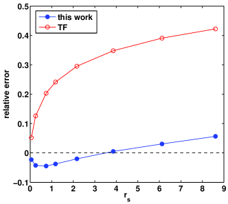
Figure 1: (color online) Relative error in the total energy calculated with our functional (filled circles) and with the Thomas-Fermi approximation (open circles) for a six-electron parabolic quantum dot as a function of the density parameter $r_{s}$.

shows the relative error of our functional (filled circles) and the TF approximation (open circles) in the total energy against the reference LDA result, i.e., $|E_{\rm LDA}-E|/E_{\rm LDA}$. We emphasize that for this system the relative error of the reference LDA is below $0.003$ with respect to quantum Monte Carlo calculations. lda The values used for $r_{s}$ correspond to a wide range of the interaction strength, covering well the typical values ($r_{s}\sim 1\ldots 5$) used when modeling QD’s within the effective-mass approximation at the interface of GaAs and AlGaAs. jacak ; reimann_rmp ; kouwenhoven

Overall, we find an excellent agreement in the total energies between the LDA and our functional. The relative error remains below $\sim 5\,\%$ through the full range of $r_{s}$. On the other hand, the TF approximation is accurate only close to the noninteracting limit ($r_{s}\rightarrow 0$), whereas in general the TF error is dozens of percent. The overestimation of the total energy in the TF approximation is plausible due to the lack of exchange and correlation energies which are both always negative.

Next we focus on the rectangular QS and vary both $r_{s}$ and $N$. The results are given in Fig. 2

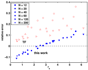
Figure 2: (color online) Relative error in the total energy calculated with our functional (filled symbols) and with the Thomas-Fermi approximation (open symbols) for rectangular quantum slabs with $N=12\ldots 200$ as a function of the density parameter $r_{s}$.

which, similarly to Fig. 1, shows the relative total-energy errors of our functional (filled symbols) and the TF (open symbols). The electron number varies in the range $N=12\ldots 200$. As in the case of a parabolic QD, the accuracy of our functionals is superior to that of the TF, except at small $r_{s}$.

A significant feature in Fig. 2 is the consistency of the accuracy of the present functional with $N$. Instead, the validity of the TF approximation strongly depends on the electron number, which is due to the fact that at fixed $r_{s}$, the relative amount of (classical) Hartree energy of the total energy increases with $N$. However, even at large electron numbers our functional is considerably more accurate than the TF approximation, on condition that the system is not too close to the noninteracting (small-$r_{s}$) regime. For example, at $N=120$ and $r_{s}\sim 3.3$, the relative errors of the present functional and the TF approximation are $2\,\%$ and $10\,\%$, respectively. Hence, our functional is expected to be a reliable tool for total-energy calculations in systems that are computationally not reachable by, e.g., the LDA (see, e.g., Ref. afif, ). In fact, the $N=200$ case in Fig. 2 was close to the numerical limit of our LDA calculations.

We observed numerically that in QD’s the difference between $T_{\rm TF}$ and $T_{\rm KS}$ is very small. As it is known, it actually goes to zero in the limit $r_{s}\rightarrow 0$ (Ref. Brack, ). In QS’s, on the other hand, $T_{\rm TF}$ may largely underestimate $T_{\rm KS}$. However, the relative contribution of this underestimation to the total energy strongly decreases as a function of $N$. It remains to be seen whether a fully self-consistent application of the presented functional may be carried out providing either accurate or at least better densities than the Thomas-Fermi ones.

V Conclusions

In summary, we have derived an explicit density functional for the total energy of electrons in two dimensions. The functional is numerically highly efficient due to the freedom from orbitals and from the calculation of the Hartree integral. When applied to models of semiconductor quantum dots and slabs up to hundreds of electrons, and up to strong electron-electron interactions, we have found a good overall agreement with respect to the local-density approximation, and a significant improvement over the Thomas-Fermi approximation. Natural future developments of the present work include the spin-dependent generalization and the capability to deal with dimensional crossovers (such as from two to three dimensions, or from two to one dimension).

- (1) For an overview, see e.g., L. Jacak, P. Hawrylak, and A. Wójs, Quantum dots (Springer, Berlin, 1998).
- (2) For a review, see, e.g., R. G. Parr and W. Yang, Density-functional Theory of Atoms and Molecules (Oxford University Press - New York, Clarendon Press, Oxford, 1989); R. M. Dreizler and E. K. U. Gross, Density functional theory (Springer, Berlin, 1990).
- (3) A. K. Rajagopal and J. C. Kimball, Phys. Rev. B 15, 2819 (1977).
- (4) B. Tanatar, D. M. Ceperley, Phys. Rev. B 39, 5005 (1989).
- (5) C. Attaccalite, S. Moroni, P. Gori-Giorgi, G.B. Bachelet, Phys. Rev. Lett. 88, 256601 (2002).
- (6) S. M. Reimann and M. Manninen, Rev. Mod. Phys. 74, 1283 (2002).
- (7) S. Pittalis, E. Räsänen, N. Helbig, and E. K. U. Gross, Phys. Rev. B 76, 235314 (2007); S. Pittalis, E. Räsänen, J. G. Vilhena, and M. A. L. Marques, Phys. Rev. A 79 012503 (2009); E. Räsänen, S. Pittalis, C. R. Proetto, and E. K. U. Gross, Phys. Rev. B 79, 121305(R) (2009); S. Pittalis, E. Räsänen, and E. K. U. Gross, Phys. Rev. A 80, 032515 (2009).
- (8) S. Pittalis, E. Räsänen, and M. A. L. Marques, Phys. Rev. B 78, 195322 (2008).
- (9) S. Pittalis, E. Räsänen, C. R. Proetto, and E. K. U. Gross, Phys. Rev. B 79, 085316 (2009).
- (10) Y. A. Wang and E. A. Carter, in Theoretical Methods in Condensed Phase Chemistry, edited by S. D. Schwartz, Progress in Theoretical Chemistry and Physics Series (Kluwer, Dordrecht, 2000), pp. 117-184.
- (11) V. L. Lignéres and E. A. Carter, An Introduction to Orbital- Free Density Functional Theory (Springer, Netherlands, 2005), and references therein.
- (12) S. C. Watson and E. A. Carter, Comput. Phys. Commun. 128, 67 (2000).
- (13) E. H. Lieb, Rev. Mod. Phys. 53, 603 (1981); ibid 54, 311 (1982).
- (14) E. H. Lieb, J. P. Solovej, and J. Yngvason, Phys. Rev. B 51, 10646 (1995).
- (15) See, e.g., A. Siddiki and R. R. Gerhardts, Phys. Rev. B 68, 125315 (2003); A. Siddiki and F. Marquardt, Phys. Rev. B 75, 045325 (2007), and references therein.
- (16) R. G. Parr, J. Phys. Chem. 92, 3060 (1988).
- (17) P. Gori-Giorgi, S. Moroni, and G. B. Bachelet, Phys. Rev. B 70, 115102 (2004).
- (18) In the 3D case, see, e.g., P. Gori-Giorgi and J. P. Perdew, Phys. Rev. B 64, 155102 (2001).
- (19) M. Brack and B. P. van Zyl, Phys. Rev. Lett. 86, 1574 (2001).
- (20) A. Holas, P. M. Kozlowski, and N. H. March, J. Phys. A: Math. Gen. 24, 4249 (1991).
- (21) L. Salasnich, J. Phys. A: Math. Theor. 40, 9987 (2007).
- (22) The situation differs for the case of fermions with spatially varying effective mass, see, K. Berkane and K. Bencheikh, Phys. Rev. A 72, 022508 (2005).
- (23) C. F. von Weizsäcker, Z. Phys. 96, 431 (1935).
- (24) M. Koskinen, M. Manninen, and S. M. Reimann, Phys. Rev. Lett. 79, 1389 (1997).
- (25) E. Räsänen, H. Saarikoski, V. N. Stavrou, A. Harju, M. J. Puska, and R. M. Nieminen, Phys. Rev. B 67, 235307 (2003).
- (26) E. Räsänen, A. Harju, M. J. Puska, and R. M. Nieminen, Phys. Rev. B 69, 165309 (2004).
- (27) H. Saarikoski, E. Räsänen, S. Siljamäki, A. Harju, M. J. Puska, and R. M. Nieminen, Phys. Rev. B 67, 205327 (2003).
- (28) N. Helbig, S. Kurth, S. Pittalis, E. Räsänen, and E. K. U. Gross, Phys. Rev. B 77, 245106 (2008).
- (29) A. Castro, H. Appel, M. Oliveira, C. A. Rozzi, X. Andrade, F. Lorenzen, M. A. L. Marques, E. K. U. Gross, and A. Rubio, Phys. Stat. Sol. (b) 243, 2465 (2006).
- (30) L. P. Kouwenhoven, D. G. Austing, and S. Tarucha, Rep. Prog. Phys. 64, 701 (2001).