Radon needlet thresholding

Abstract

We provide a new algorithm for the treatment of the noisy inversion of the Radon transform using an appropriate thresholding technique adapted to a well-chosen new localized basis. We establish minimax results and prove their optimality. In particular, we prove that the procedures provided here are able to attain minimax bounds for any $\mathbb{L}_{p}$ loss. It is important to notice that most of the minimax bounds obtained here are new to our knowledge. It is also important to emphasize the adaptation properties of our procedures with respect to the regularity (sparsity) of the object to recover and to inhomogeneous smoothness. We perform a numerical study that is of importance since we especially have to discuss the cubature problems and propose an averaging procedure that is mostly in the spirit of the cycle spinning performed for periodic signals.

, and

1 Introduction

We consider the problem of inverting noisy observations of the $d$-dimensional Radon transform. Obviously, the most immediate examples occur for $d=2$ or 3. However, no major differences arise from considering the general case.

There is considerable literature on the problem of reconstructing structures from their Radon transforms, which is a fundamental problem in medical imaging and, more generally, in tomography. In our approach, we focus on several important points. We produce a procedure that is efficient from an $\mathbb{L}_{2}$ point of view, since this loss function mimics quite well in many situations the preferences of the human eye. On the other hand, we have at the same time the requirement of clearly identifying the local bumps, of being able to estimate the different level sets well. We also want the procedure to enjoy good adaptation properties. In addition, we require the procedure to be simple to implement.

At the heart of such a problem, there is a notable conflict between the inversion part – which, in the presence of noise, creates an instability reasonably handled by a singular value decomposition (SVD) approach – and the fact that the SVD basis is very rarely localized and, as a consequence, capable of representing local features of images, which are especially important to recover.

Our strategy is to follow the approach started in [11], which utilizes a construction borrowed from [21] (see also [13]) of localized frames based on orthogonal polynomials on the ball, which are closely related to the Radon transform SVD basis.

To achieve the goals presented above, and especially adaptation to different regularities and local inhomogeneous smoothness, we add a fine-tuned subsequent thresholding process to the estimation performed in [11].

This improves considerably the performances of the algorithm, both from a theoretical point of view and a numerical point of view. In effect, the new algorithm provides a much better spatial adaptation, as well as adaptation to the classes of regularity. We prove here that the bounds obtained by the procedure are minimax over a large class of Besov spaces and any $\mathbb{L}_{p}$ loss: we provide upper bounds for the performance of our algorithm and lower bounds for the associated minimax rate.

It is important to notice that because we consider different $\mathbb{L}_{p}$ losses, we provide rates of convergence of new types attained by our procedure. Those rates are minimax since they are confirmed by lower-bound inequalities.

The problem of choosing appropriate spaces of regularity on the ball reflecting the standard objects analyzed in tomography is a highly non-trivial problem. We decided to consider the spaces that seem to stay closest to our natural intuition, that is, those that generalize to the ball the approximation properties by polynomials.

The procedure gives very promising results in the simulation study. We show that the estimates obtained by thresholding the needlets outperform those obtained either by thresholding the SVD or by the linear needlet estimate proposed in [11]. An important issue in the needlet scheme is the choice of the quadrature in the needlet construction. We discuss the possibilities proposed in the literature and consider a cubature formula based on the full tensorial grid on the sphere, introducing an averaging close to the cycle-spinning method.

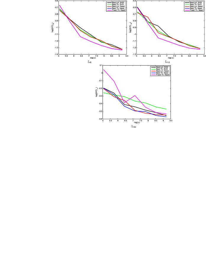
Figure 5: Estimation results in log $\mathbb{L}_{p}$ norm. Each figure shows the decay of the logarithm of the error against the logarithm of the noise parameter for the specified norm.

Among others, one amazing result is that, to attain minimax rates in the $\mathbb{L}_{\infty}$ norm, we need to modify the estimator. This result is also corroborated by the numerical results: see Theorem 2 and Figures 4 and 5.

In the first section, we introduce the Radon transform and the associated SVD basis. The following section summarizes the construction of the localized basis, the needlets. The procedure is introduced in Section 4, where the main theoretical results are stated for upper bounds and lower bounds. Section 5 details the simulation study. Section 6 details important properties of the needlet basis. The proof of the two main results stated in Section 4 is postponed in the two last sections.

2 Radon transform and white noise model

2.1 Radon transform

Here we recall the definitions and some basic facts about the Radon transform (cf. [10, 19, 14]). Denote by $B^{d}$ the unit ball in ${\mathbb{R}}^{d}$, that is, $B^{d}=\{x=(x_{1},\ldots,x_{d})\in{\mathbb{R}}^{d}\colon\ |x|\leq 1\}$ with $|x|=(\sum_{i=1}^{d}x_{i}^{2})^{1/2}$ and, by $\mathbb{S}^{d-1}$, the unit sphere in ${\mathbb{R}}^{d}$. The Lebesgue measure on $B^{d}$ will be denoted by $\mathrm{d}x$ and the usual surface measure on $\mathbb{S}^{d-1}$ by $\mathrm{d}\sigma(x)$ (sometimes we will also deal with the surface measure on $\mathbb{S}^{d}$, which will be denoted by $\mathrm{d}\sigma_{d}$). We let $|A|$ denote the measure $|A|=\int_{A}\mathrm{d}x$ if $A\subset B^{d}$ and $|A|=\int_{A}\mathrm{d}\sigma(x)$ if $A\subset\mathbb{S}^{d-1}$.

The Radon transform of a function $f$ is defined by

$$Rf(\theta,s)=\int_{\mathop{y\in\theta^{\perp}}\limits_{s\theta+y\in B^{d}}}f(s\theta+y)\,\mathrm{d}y,\qquad\theta\in\mathbb{S}^{d-1},s\in[-1,1],$$

where $\mathrm{d}y$ is the Lebesgue measure of dimension $d-1$ and $\theta^{\perp}=\{x\in{\mathbb{R}}^{d}\colon\ \langle x,\theta\rangle=0\}$. With a slight abuse of notation, we will rewrite this integral as

$$Rf(\theta,s)=\int_{\langle y,\theta\rangle=s}f(y)\,\mathrm{d}y.$$

By Fubini’s theorem, we have

$$\int_{-1}^{1}Rf(\theta,s)\,\mathrm{d}s=\int_{B^{d}}f(x)\,\mathrm{d}x.$$

It is easy to see (cf. [19]) that the Radon transform is a bounded linear operator mapping $\mathbb{L}_{2}(B^{d},\mathrm{d}x)$ into $\mathbb{L}_{2}(\mathbb{S}^{d-1}\times[-1,1],\mathrm{d}\mu(\theta,s))$, where

$$\mathrm{d}\mu(\theta,s)=\mathrm{d}\sigma(\theta)\frac{\mathrm{d}s}{(1-s^{2})^{(d-1)/2}}.$$

2.2 Noisy observation of the Radon transform

We consider observations of the form

$$\mathrm{d}Y(\theta,s)=Rf(\theta,s)\,\mathrm{d}\mu(\theta,s)+\varepsilon\,\mathrm{d}W(\theta,s),$$

where the unknown function $f$ belongs to $\mathbb{L}_{2}(B^{d},\mathrm{d}x)$. The meaning of this equation is that, for any $\varphi(\theta,s)$ in $\mathbb{L}_{2}(\mathbb{S}^{d-1}\times[-1,1],\mathrm{d}\mu(\theta,s)),$ one can observe

$$Y_{\varphi} = \int\varphi(\theta,s)\,\mathrm{d}Y(\theta,s)=\int_{\mathbb{S}^{d-1}\times[-1,1]}Rf(\theta,s)\varphi(\theta,s)\,\mathrm{d}\mu(\theta,s)+\varepsilon\int\varphi(\theta,s)\,\mathrm{d}W(\theta,s)$$

$$= \langle Rf,\varphi\rangle_{\mu}+\varepsilon W_{\varphi}.$$

Here $W_{\varphi}=\int\varphi(\theta,s)\,\mathrm{d}W(\theta,s)$ is a Gaussian field of zero mean and covariance

$$\mathbb{E}(W_{\varphi},W_{\psi})=\int_{\mathbb{S}^{d-1}\times[-1,1]}\varphi(\theta,s)\psi(\theta,s)\,\mathrm{d}\sigma(\theta)\frac{\mathrm{d}s}{(1-s^{2})^{(d-1)/2}}=\langle\varphi,\psi\rangle_{\mu}.$$

The goal is to recover the unknown function $f$ from the observation of $Y$. Our idea is to refine the algorithms proposed in [11] using thresholding methods. In [11], estimation schemes are derived that combine the stability and computability of SVD decompositions with the localization and multiscale structure of wavelets. To this end, a specific frame (essentially following the construction from [13]) is used. It comprises elements of nearly exponential localization and is, in addition, compatible with the SVD basis of the Radon transform.

2.3 Singular value decomposition of the Radon transform

The SVD of the Radon transform was first established in [5, 15]. In this regard, we also refer the reader to [19, 28].

2.3.1 Jacobi and Gegenbauer polynomials

The Radon SVD bases are defined in terms of Jacobi and Gegenbauer polynomials. The Jacobi polynomials $P_{n}^{(\alpha,\beta)}$, $n\geq 0$, constitute an orthogonal basis for the space $\mathbb{L}_{2}([-1,1],w_{\alpha,\beta}(t)\,\mathrm{d}t)$ with weight $w_{\alpha,\beta}(t)=(1-t)^{\alpha}(1+t)^{\beta}$, $\alpha,\beta>-1$. They are standardly normalized by $P_{n}^{(\alpha,\beta)}(1)={{n+\alpha\choose n}}$ and then [1, 7, 25]

$$\int_{-1}^{1}P_{n}^{(\alpha,\beta)}(t)P_{n^{\prime}}^{(\alpha,\beta)}(t)w_{\alpha,\beta}(t)\,\mathrm{d}t=\delta_{n,n^{\prime}}h_{n}^{(\alpha,\beta)},$$

where

$$h_{n}^{(\alpha,\beta)}=\frac{2^{\alpha+\beta+1}}{(2n+\alpha+\beta+1)}\frac{\Gamma(n+\alpha+1)\Gamma(n+\beta+1)}{\Gamma(n+1)\Gamma(n+\alpha+\beta+1)}.$$

The Gegenbauer polynomials $C_{n}^{\lambda}$ are a particular case of Jacobi polynomials and are traditionally defined by

$$C_{n}^{\lambda}(t)=\frac{(2\lambda)_{n}}{(\lambda+1/2)_{n}}P_{n}^{(\lambda-1/2,\lambda-1/2)}(t),\qquad\lambda>-1/2,$$

where, by definition, $(a)_{n}=a(a+1)\cdots(a+n-1)=\frac{\Gamma(a+n)}{\Gamma(a)}$ (note that in [25] the Gegenbauer polynomial $C_{n}^{\lambda}$ is denoted by $P_{n}^{\lambda}$). It is readily seen that $C_{n}^{\lambda}(1)={n+2\lambda-1\choose n}=\frac{\Gamma(n+2\lambda)}{n!\Gamma(2\lambda)}$ and

$$\int_{-1}^{1}C^{\lambda}_{n}(t)C^{\lambda}_{m}(t)(1-t^{2})^{\lambda-1/2}\,\mathrm{d}t=\delta_{n,m}h_{n}^{(\lambda)}\qquad\mbox{with }h_{n}^{(\lambda)}=\frac{2^{1-2\lambda}\pi}{\Gamma(\lambda)^{2}}\frac{\Gamma(n+2\lambda)}{(n+\lambda)\Gamma(n+1)}.$$

2.3.2 Polynomials on $B^{d}$ and $\mathbb{S}^{d-1}$

Let $\Pi_{n}({\mathbb{R}}^{d})$ be the space of all polynomials in $d$ variables of degree $\leq n$. We denote by ${\cal P}_{n}({\mathbb{R}}^{d})$ the space of all homogeneous polynomials of degree $n$ and by ${\cal V}_{n}({\mathbb{R}}^{d})$ the space of all polynomials of degree $n$ that are orthogonal to lower-degree polynomials with respect to the Lebesgue measure on $B^{d}$. Of course, ${\cal V}_{0}({\mathbb{R}}^{d})$ will be the set of all constants. We have the following orthogonal decomposition:

$$\Pi_{n}({\mathbb{R}}^{d})=\bigoplus_{k=0}^{n}{\cal V}_{k}({\mathbb{R}}^{d}).$$

Also, denote by ${\mathbb{H}}_{n}({\mathbb{R}}^{d})$ the subspace of all harmonic homogeneous polynomials of degree $n$ (i.e., $Q\in{\mathbb{H}}_{n}({\mathbb{R}}^{d})$ if $Q\in{\cal P}_{n}({\mathbb{R}}^{d})$ and $\Delta Q=0$) and, by ${\mathbb{H}}_{n}(\mathbb{S}^{d-1}),$ the (injective) restriction of the polynomials from ${\mathbb{H}}_{n}({\mathbb{R}}^{d})$ to $\mathbb{S}^{d-1}$. It is well known that

$$N_{d-1}(n)=\dim({\mathbb{H}}_{n}(\mathbb{S}^{d-1}))=\pmatrix{n+d-1\cr d-1}-\pmatrix{n+d-3\cr d-1}\sim n^{d-2}.$$

Let $\Pi_{n}(\mathbb{S}^{d-1})$ be the space of restrictions to $\mathbb{S}^{d-1}$ of polynomials of degree $\leq n$ on ${\mathbb{R}}^{d}$. It is also well known that

$$\Pi_{n}(\mathbb{S}^{d-1})=\bigoplus_{m=0}^{n}{\mathbb{H}}_{m}(\mathbb{S}^{d-1})$$

(the orthogonality is, with respect to the surface measure, $\mathrm{d}\sigma$ on $\mathbb{S}^{d-1}$). ${\mathbb{H}}_{l}(\mathbb{S}^{d-1})$ is called the space of spherical harmonics of degree $d$ on the sphere $\mathbb{S}^{d-1}$.

Let $Y_{l,m}$, $1\leq m\leq N_{d-1}(l)$, be an orthonormal basis of ${\mathbb{H}}_{l}(\mathbb{S}^{d-1})$, that is,

$$\int_{\mathbb{S}^{d-1}}Y_{l,m}(\xi)\overline{Y_{l,m^{\prime}}(\xi)}\,\mathrm{d}\sigma(\xi)=\delta_{m,m^{\prime}}.$$

Then the natural extensions of $Y_{l,m}$ on $B^{d}$ are defined by $Y_{l,m}(x)=|x|^{l}Y_{l,m}(\frac{x}{|x|})$ and satisfy

$$\int_{B^{d}}Y_{l,m}(x)\overline{Y_{l,m^{\prime}}(x)}\,\mathrm{d}x = \int_{0}^{1}r^{d-1}\int_{\mathbb{S}^{d-1}}Y_{l,m}(r\xi)\overline{Y_{l,m^{\prime}}(r\xi)}\,\mathrm{d}\sigma(\xi)\,\mathrm{d}r$$

$$= \int_{0}^{1}r^{d+2l-1}\int_{\mathbb{S}^{d-1}}Y_{l,m}(\xi)\overline{Y_{l,m^{\prime}}(\xi)}\,\mathrm{d}\sigma(\xi)\,\mathrm{d}r=\delta_{m,m^{\prime}}\frac{1}{2l+d}.$$

For more details, we refer the reader to [6].

The spherical harmonics on $\mathbb{S}^{d-1}$ and orthogonal polynomials on $B^{d}$ are naturally related to Gegenbauer polynomials. Thus, the kernel of the orthogonal projector onto ${\mathbb{H}}_{n}(\mathbb{S}^{d-1})$ can be written as (see [24]):

$$\sum_{m=1}^{N_{d-1}(n)}Y_{l,m}(\xi)\overline{Y_{l,m}(\theta)}=\frac{2n+d-2}{(d-2)|\mathbb{S}^{d-1}|}C^{{(d-2)/2}}_{n}(\langle\xi,\theta\rangle).$$ (1)

The “ridge” Gegenbauer polynomials $C_{n}^{d/2}(\langle x,\xi\rangle)$ are orthogonal to $\Pi_{n-1}(B^{d})$ in $\mathbb{L}_{2}(B^{d})$ and the kernel $L_{n}(x,y)$ of the orthogonal projector onto ${\cal V}_{n}(B^{d})$ can be written in the form (see [22, 28])

$$L_{n}(x,y) = \frac{2n+d}{|\mathbb{S}^{d-1}|^{2}}\int_{\mathbb{S}^{d-1}}C^{d/2}_{n}(\langle x,\xi\rangle)C^{d/2}_{n}(\langle y,\xi\rangle)\,\mathrm{d}\sigma(\xi)$$

$$= \frac{(n+1)_{d-1}}{2^{d}\uppi^{d-1}}\int_{\mathbb{S}^{d-1}}\frac{C^{d/2}_{n}(\langle x,\xi\rangle)C^{d/2}_{n}(\langle y,\xi\rangle)}{\|C^{d/2}_{n}\|^{2}}\,\mathrm{d}\sigma(\xi).$$

The following important identities are valid for “ridge” Gegenbauer polynomials:

$$\int_{B^{d}}C^{d/2}_{n}(\langle\xi,x\rangle)C^{d/2}_{n}(\langle\eta,x\rangle)\,\mathrm{d}x=\frac{h_{n}^{(d/2)}}{C_{n}^{d/2}(1)}C^{d/2}_{n}(\langle\xi,\eta\rangle),\qquad\xi,\eta\in\mathbb{S}^{d-1},$$ (3)

and, for $x\in B^{d}$, $\eta\in\mathbb{S}^{d-1}$,

$$\int_{\mathbb{S}^{d-1}}C^{d/2}_{n}(\langle\xi,x\rangle)C^{d/2}_{n}(\langle\xi,\eta\rangle)\,\mathrm{d}\sigma(\xi)=|\mathbb{S}^{d-1}|C^{d/2}_{n}(\langle\eta,x\rangle);$$ (4)

see [22]. By (2.3.2) and (4)

$$L_{n}(x,\xi)=\frac{(2n+d)}{|\mathbb{S}^{d-1}|}C^{d/2}_{n}(\langle x,\xi\rangle),\qquad\xi\in\mathbb{S}^{d-1},$$

and again by (2.3.2)

$$\int_{\mathbb{S}^{d-1}}L_{n}(x,\xi)L_{n}(y,\xi)\,\mathrm{d}\sigma(\xi)=(2n+d)L_{n}(x,y).$$

2.3.3 The SVD of the Radon transform

Assume that $\{Y_{l,m}\colon\ 1\leq m\leq N_{d-1}(l)\}$ is an orthonormal basis for ${\mathbb{H}}_{l}(\mathbb{S}^{d-1})$. Then it is standard and easy to see that the family of polynomials,

$$f_{k,l,m}(x)=(2k+d)^{1/2}P_{j}^{(0,l+d/2-1)}(2|x|^{2}-1)Y_{l,m}(x),$$

$$\quad 0\leq l\leq k,k-l=2j,1\leq i\leq N_{d-1}(l),$$

form an orthonormal basis of ${\cal V}_{k}(B^{d})$; see [6]. Here, as before, $Y_{l,m}(x)=|x|^{l}Y_{l,m}(x/|x|)$. On the other hand, the collection

$$g_{k,l,m}(\theta,s)=\bigl{[}h_{k}^{(d/2)}\bigr{]}^{-1/2}(1-s^{2})^{(d-1)/2}C^{d/2}_{k}(s)Y_{l,m}(\theta),\qquad k\geq 0,l\geq 0,1\leq m\leq N_{d-1}(l),$$

is an orthonormal basis of $\mathbb{L}_{2}(\mathbb{S}^{d-1}\times[-1,1],\mathrm{d}\mu(\theta,s))$. Most important, the Radon transform $R\mathchoice{\nobreak\,\colon}{\nobreak\,\colon}{\nobreak\,\colon\;}{\nobreak\,\colon\;}\mathbb{L}_{2}(B^{d})\mapsto\mathbb{L}_{2}(\mathbb{S}^{d-1}\times[-1,1],\mathrm{d}\mu(\theta,s))$ is a one-to-one mapping and

$$Rf_{k,l,m}=\lambda_{k}g_{k,l,m},\qquad R^{*}g_{k,l,m}=\lambda_{k}f_{k,l,m},$$

where

$$\lambda_{k}^{2}=\frac{2^{d}\pi^{d-1}}{(k+1)(k+2)\cdots(k+d-1)}=\frac{2^{d}\pi^{d-1}}{(k+1)_{d-1}}\sim k^{-d+1}.$$

More precisely, we have for any $f\in\mathbb{L}_{2}(B^{d})$

$$Rf=\sum_{k\geq 0}\lambda_{k}\sum_{0\leq l\leq k,k-l\equiv 0\ (\operatorname{mod}2)}\sum_{1\leq m\leq N_{d-1}(l)}\langle f,f_{k,l,m}\rangle g_{k,l,m}.$$

Furthermore, for $f\in\mathbb{L}_{2}(B^{d}),$

$$f=\sum_{k\geq 0}\lambda_{k}^{-1}\sum_{0\leq l\leq k,k-l\equiv 0\ (\operatorname{mod}2)}\sum_{1\leq m\leq N_{d-1}(l)}\langle Rf,g_{k,l,m}\rangle_{\mu}f_{k,l,m}.$$

In the above identities, the convergence is in $\mathbb{L}_{2}$.

For the Radon SVD, we refer the reader to [19, 28, 11].

3 Construction of needlets on the ball

In this section, we briefly recall the construction of the needlets on the ball. This construction is due to [21]. Its aim is to build a very well-localized tight frame constructed using the eigenvectors of the Radon transform. For more precision, we refer the reader to [21, 12, 11]

Let $\{f_{k,l,m}\}$ be the orthonormal basis of ${\cal V}_{k}(B^{d})$ defined in Section 2.3.3. Denote by $T_{k}$ the index set of this basis, that is, $T_{k}=\{(l,m)\colon\ 0\leq l\leq k,l\equiv k\ (\operatorname{mod}2),0\leq m\leq N_{d-1}(l)\}$. Then the orthogonal projector of $\mathbb{L}_{2}(B^{d})$ onto ${\cal V}_{k}(B^{d})$ can be written in the form

$$L_{k}f=\int_{B^{d}}f(y)L_{k}(x,y)\,\mathrm{d}y\qquad\mbox{with }L_{k}(x,y)=\sum_{l,m\in T_{k}}f_{k,l,m}(x)f_{k,l,m}(y).$$

Using (1), $L_{k}(x,y)$ can be written in the form

$$L_{k}(x,y)$$

$$\quad=(2k+d)\sum_{l\leq k,k-l\equiv 0\ (\operatorname{mod}2)}P_{j}^{(0,l+d/2-1)}(2|x|^{2}-1)|x|^{l}P_{j}^{(0,l+d/2-1)}(2|y|^{2}-1)|y|^{l}$$

$$\hphantom{=(2k+d)\sum_{l\leq k,k-l\equiv 0\ (\operatorname{mod}2)}}\quad{}\times\sum_{m}Y_{l,m}\biggl{(}\frac{x}{|x|}\biggr{)}Y_{l,m}\biggl{(}\frac{y}{|y|}\biggr{)}$$

$$\quad=\frac{(2k+d)}{|\mathbb{S}^{d-1}|}\sum_{l\leq k,k-l\equiv 0\ (\operatorname{mod}2)}P_{j}^{(0,l+d/2-1)}(2|x|^{2}-1)|x|^{l}P_{j}^{(0,l+d/2-1)}(2|y|^{2}-1)|y|^{l}$$

$$\hphantom{=\frac{(2k+d)}{|\mathbb{S}^{d-1}|}\sum_{l\leq k,k-l\equiv 0\ (\operatorname{mod}2)}}\quad{}\times\biggl{(}1+\frac{l}{d/2-1}\biggr{)}C^{d/2-1}_{l}\biggl{(}\biggl{\langle}\frac{x}{|x|},\frac{y}{|y|}\biggr{\rangle}\biggr{)}.$$

Another representation of $L_{k}(x,y)$ has already been given in (2.3.2). Clearly,

$$\int_{B^{d}}L_{k}(x,z)L_{k^{\prime}}(z,y)\,\mathrm{d}z=\delta_{k,k^{\prime}}L_{k}(x,y)$$ (5)

and, for $f\in\mathbb{L}_{2}(B^{d}),$

$$f=\sum_{k\geq 0}L_{k}f\quad\mbox{and}\quad\|f\|_{2}^{2}=\sum_{k}\|L_{k}f\|_{2}^{2}=\sum_{k}\langle L_{k}f,f\rangle.$$ (6)

The construction of the needlets is based on the classical Littlewood–Paley decomposition and a subsequent discretization.

Let $a\in C^{\infty}[0,\infty)$ be a cut-off function such that $0\leq a\leq 1$, $a(t)=1$ for $t\in[0,1/2]$ and $\operatorname{supp}a\subset[0,1]$. We next use this function to introduce a sequence of operators on $\mathbb{L}_{2}(B^{d})$. For $j\geq 0$, write

$$A_{j}f(x)=\sum_{k\geq 0}a\biggl{(}\frac{k}{2^{j}}\biggr{)}L_{k}f(x)=\int_{B^{d}}A_{j}(x,y)f(y)\,\mathrm{d}y$$

$$\quad\mbox{with }A_{j}(x,y)=\sum_{k}a\biggl{(}\frac{k}{2^{j}}\biggr{)}L_{k}(x,y).$$

Also, we define $B_{j}f=A_{j+1}f-A_{j}f$. Then, setting $b(t)=a(t/2)-a(t),$ we have

$$B_{j}f(x)=\sum_{k}b\biggl{(}\frac{k}{2^{j}}\biggr{)}L_{k}f(x)=\int_{B^{d}}B_{j}(x,y)f(y)\,\mathrm{d}y$$

$$\quad\mbox{with }B_{j}(x,y)=\sum_{k}b\biggl{(}\frac{k}{2^{j}}\biggr{)}L_{k}(x,y).$$

Obviously, for $f\in\mathbb{L}_{2}(B^{d})$,

$$\langle A_{j}f,f\rangle=\sum_{k}a\biggl{(}\frac{k}{2^{j}}\biggr{)}\langle L_{k}f,f\rangle\leq\|f\|_{2}^{2}.$$

An important result from [21] (cf. [13]) asserts that the kernels $A_{j}(x,y)$, $B_{j}(x,y)$ have nearly exponential localization. Namely, for any $M>0$ there exists a constant $C_{M}>0$ such that

$$|A_{j}(x,y)|,|B_{j}(x,y)|\leq C_{M}\frac{2^{jd}}{(1+2^{j}d(x,y))^{M}\sqrt{W_{j}(x)}\sqrt{W_{j}(y)}},\qquad x,y\in B^{d},$$ (7)

where

$$W_{j}(x)=2^{-j}+\sqrt{1-|x|^{2}},\qquad|x|^{2}=|x|^{2}_{d}=\sum_{i=1}^{d}x_{i}^{2}$$ (8)

and

$$d(x,y)=\operatorname{Arccos}\bigl{(}\langle x,y\rangle+\sqrt{1-|x|^{2}}\sqrt{1-|y|^{2}}\bigr{)},\qquad\langle x,y\rangle=\sum_{i=1}^{d}x_{i}y_{i}.$$

Let us define

$$C_{j}(x,y)=\sum_{k}\sqrt{a\biggl{(}\frac{k}{2^{j}}\biggr{)}}L_{k}(x,z)\quad\mbox{and}\quad D_{j}(x,y)=\sum_{k}\sqrt{b\biggl{(}\frac{k}{2^{j}}\biggr{)}}L_{k}(x,z).$$

Note that $C_{j}$ and $D_{j}$ have the same localization as the localization of $A_{j}$, $B_{j}$ in (7) (cf. [21]). Using (5), we get,

$$A_{j}(x,y)=\int_{B^{d}}C_{j}(x,z)C_{j}(z,y)\,\mathrm{d}z,\qquad B_{j}(x,y)=\int_{B^{d}}D_{j}(x,z)D_{j}(z,y)\,\mathrm{d}z.$$ (9)

And, obviously, $z\mapsto C_{j}(x,z)C_{j}(z,y)$ (resp., $D_{j}(x,z)D_{j}(z,y)$) are polynomial of degrees $<2^{j+1}$.

The following proposition follows from results in [21] and [27] and establishes a cubature formula.

Proposition 1

Let $\{B(\widetilde{\xi}_{i},\rho)\colon\ i\in I\}$ be a maximal family of disjoint spherical caps of radius $\rho=\tau 2^{-j}$ with centers on the hemisphere $\mathbb{S}_{+}^{d}$. Then for sufficiently small $0<\tau\leq 1$ the set of points $\chi_{j}=\{\xi_{i}\colon\ i\in I\}$ obtained by projecting the set $\{\widetilde{\xi}\colon\ i\in I\}$ on $B^{d}$ is a set of nodes of a cubature formula that is exact for $\Pi_{2^{j+2}}(B^{d})$: for any $P\in\Pi_{2^{j+2}}(B^{d})$,

$$\int_{B^{d}}P(u)\,\mathrm{d}u=\sum_{\xi\in\chi_{j}}\omega_{j,\xi}P(\xi),$$

where, moreover, the coefficients $\omega_{j,\xi}$ of this cubature are positive and satisfy $\omega_{j,\xi}\sim W_{j}(\xi)2^{-jd}$, and the cardinality of the set $\chi_{j}$ is of order $2^{jd}$.

3.1 Needlets

Going back to identities (9) and applying the cubature formula described in Proposition 1, we get

$$A_{j}(x,y) = \int_{B^{d}}C_{j}(x,z)C_{j}(z,y)\,\mathrm{d}z=\sum_{\xi\in\chi_{j}}\omega_{j,\xi}C_{j}(x,\xi)C_{j}(y,\xi)\quad\mbox{and}$$

$$B_{j}(x,y) = \int_{B^{d}}D_{j}(x,z)D_{j}(z,y)\,\mathrm{d}z=\sum_{\xi\in\chi_{j}}\omega_{j,\xi}D_{j}(x,\xi)D_{j}(y,\xi).$$

We define the father needlets, $\varphi_{j,\xi}$, and the mother needlets, $\psi_{j,\xi}$, by

$$\varphi_{j,\xi}(x)=\sqrt{\omega_{j,\xi}}C_{j}(x,\xi)\quad\mbox{and}\quad\psi_{j,\xi}(x)=\sqrt{\omega_{j,\xi}}D_{j}(x,\xi),\qquad\xi\in\chi_{j},j\geq 0.$$

We also set $\psi_{-1,0}=\frac{{1}_{B^{d}}}{|B^{d}|}$ and $\chi_{-1}=\{0\}$. From above, it follows that

$$A_{j}(x,y)=\sum_{\xi\in\chi_{j}}\varphi_{j,\xi}(x)\varphi_{j,\xi}(y),\qquad B_{j}(x,y)=\sum_{\xi\in\chi_{j}}\psi_{j,\xi}(x)\psi_{j,\xi}(y).$$

Therefore,

$$A_{j}f(x)=\int_{B^{d}}A_{j}(x,y)f(y)\,\mathrm{d}y=\sum_{\xi\in\chi_{j}}\langle f,\varphi_{j,\xi}\rangle\varphi_{j,\xi}=\sum_{\xi\in\chi_{j}}\alpha_{j,\xi}\varphi_{j,\xi},\qquad\alpha_{j,\xi}=\langle f,\varphi_{j,\xi}\rangle$$

and

$$B_{j}f(x)=\int_{B^{d}}B_{j}(x,y)f(y)\,\mathrm{d}y=\sum_{\xi\in\chi_{j}}\langle f,\psi_{j,\xi}\rangle\psi_{j,\xi}=\sum_{\xi\in\chi_{j}}\beta_{j,\xi}\psi_{j,\xi},\qquad\beta_{j,\xi}=\langle f,\psi_{j,\xi}\rangle.$$

It is easy to prove (see [21]) that

$$\|\varphi_{j,\xi}\|_{2}\leq 1.$$

From (6) and the fact that $\sum_{j\geq 0}b(t2^{-j})=1$ for $t\in[1,\infty)$, it readily follows that

$$f=\sum_{j\geq-1}\sum_{\xi\in\chi_{j}}\langle f,\psi_{j,\xi}\rangle\psi_{j,\xi},\qquad f\in\mathbb{L}_{2}(B^{d}),$$

and, taking the inner product with $f$, it leads to

$$\|f\|_{2}^{2}=\sum_{j}\sum_{\xi\in\chi_{j}}|\langle f,\psi_{j,\xi}\rangle|^{2}.$$

In turn, this shows that the family $\{\psi_{j,\xi}\}$ is a tight frame for $\mathbb{L}_{2}(B^{d})$.

4 Needlet inversion of a noisy Radon transform and minimax performances

Our estimator is based on an appropriate thresholding of a needlet expansion as follows. $f$ can be decomposed using the frame above:

$$f=\sum_{j\geq-1}\sum_{\xi\in\chi_{j}}\langle f,\psi_{j,\xi}\rangle\psi_{j,\xi}.$$

Our estimation procedure will be defined by the following steps

$$\widehat{\alpha}_{k,l,m} = \frac{1}{\lambda_{k}}\int g_{k,l,m}\,\mathrm{d}Y,$$ (10)

$$\widehat{\beta}_{j,\xi} = \sum_{k,l,m}\gamma^{j,\xi}_{k,l,m}\widehat{\alpha}_{k,l,m}$$ (11)

with

$$\gamma^{j,\xi}_{k,l,m}=\langle g_{k,l,m},\psi_{j,\xi}\rangle$$

and

$$\hat{f}=\sum_{j=-1}^{J_{\varepsilon}}\sum_{\xi\in\chi_{j}}\widehat{\beta}_{j,\xi}{1}_{\{|\widehat{\beta}_{j,\xi}|\geq\kappa 2^{j\nu}c_{\varepsilon}\}}\psi_{j,\xi}$$ (12)

with

$$\nu=(d-1)/2.$$ (13)

Hence, our procedure has three steps: the first one (10) corresponds to the inversion of the operator in the SVD basis, the second one (11) projects on the needlet basis and the third one (12) ends up the procedure with a final thresholding. The tuning parameters of this estimator are

• The range $J_{\varepsilon}$ of resolution levels will be taken such that

  $$2^{J_{\varepsilon}(d-{1/2})}\leq\bigl{(}\varepsilon\sqrt{\log 1/\varepsilon}\bigr{)}^{-1}<2^{(J_{\varepsilon}+1)(d-{1/2})}.$$

• The threshold constant $\kappa$ is an important tuning of our method. The theoretical point of view asserts that, for $\kappa$ above a constant (for which our evaluation is probably not optimal), the minimax properties hold. Evaluations of $\kappa$ from the simulation point of view are also given.

• $c_{\varepsilon}$ is a constant depending on the noise level. We shall see that the following choice is appropriate:

  $$c_{\varepsilon}=\varepsilon\sqrt{\log 1/\varepsilon}.$$

• Notice that the threshold function for each coefficient contains $2^{j\nu}$. This is due to the inversion of the Radon operator and the concentration relative to the $g_{k,l,m}$’s of the needlets.

• It is important to remark here that, unlike the (linear) procedures proposed in [11], this one does not require the knowledge of the regularity while, as will be seen in the sequel, it attains bounds that are as good as the linear ones and even better since they are handling much wider ranges for the parameters of the Besov spaces.

We will consider the minimax properties of this estimator on the Besov bodies constructed on the needlet basis. In [13], it is proved that these spaces can also be described as approximation spaces, so they have a genuine meaning and can be compared to standard Sobolev spaces.

We define here the Besov body, $B^{s}_{\pi,r}$, as the space of functions $f=\sum_{j\geq-1}\sum_{\xi\in\chi_{j}}\beta_{j,\xi}\psi_{j,\xi}$ such that

$$\sum_{j}2^{jsr}\biggl{(}\sum_{\xi\in\chi_{j}}(|\beta_{j,\xi}|\|\psi_{j,\xi}\|_{\pi})^{\pi}\biggr{)}^{r/\pi}<\infty$$

(with the obvious modifications for the cases $\pi$ or $r=\infty$) and $B^{s}_{\pi,r}(M),$ the ball of radius $M$ of this space.

Theorem 1

For $0<r\leq\infty$, $\pi\geq 1$, $1\leq p<\infty$, there exist some constant $c_{p}=c_{p}(s,\pi,r,M)$, $\kappa_{0}$ such that if $\kappa\geq\kappa_{0}$, $s>(d+1)(\frac{1}{\pi}-\frac{1}{p})_{+}$ and, in addition, if $\pi<p$, $s>\frac{d+1}{\pi}-\frac{1}{2}$:

(

• 3)]

• If $\frac{1}{p}<\frac{d}{d+1}$,

  $$\sup_{f\in B^{s}_{\pi,r}(M)}(\mathbb{E}\|\hat{f}-f\|_{p}^{p})^{{1/p}}$$

  $$\quad\leq c_{p}({\log 1/\varepsilon})^{{p/2}}$$

  $$\qquad{}\times\bigl{(}\varepsilon\sqrt{\log 1/\varepsilon}\bigr{)}^{{(s-(d+1)(1/\pi-1/p))/(s+d-(d+1)/\pi)}\wedge{s/(s+d-1/2)}\wedge{(s-2(1/\pi-1/p))/(s+d-2/\pi)}}.$$

• If $\frac{d}{d+1}\leq\frac{1}{p}$ and $d>2$ or $p>1$,

  $$\sup_{f\in B^{s}_{\pi,r}(M)}(\mathbb{E}\|\hat{f}-f\|_{p}^{p})^{{1/p}}\leq c_{p}({\log 1/\varepsilon})^{{p/2}}\bigl{(}\varepsilon\sqrt{\log 1/\varepsilon}\bigr{)}^{{s/(s+d-1/2)}\wedge{(s-2(1/\pi-1/p))/(s+d-2/\pi)}}.$$

• If $d=2$ and $p=1,$

  $$\sup_{f\in B^{s}_{\pi,r}(M)}(\mathbb{E}\|\hat{f}-f\|_{1})\leq c_{1}({\log 1/\varepsilon})^{{1/2}}\bigl{(}\varepsilon\sqrt{\log 1/\varepsilon}\bigr{)}^{{s/(s+2-1/2)}}.$$

Remark 0.

Up to logarithmic terms, the rates observed here are minimax, as will appear in the following theorem. It is known that in this kind of estimation, full adaptation yields unavoidable extra logarithmic terms. The rates of the logarithmic terms obtained in these theorems are, most of the time, suboptimal (for instance, for obvious reasons, the case $p=2$ yields fewer logarithmic terms). A more detailed study could lead to optimized rates, which we decided not to include here for the sake of simplicity.

The cumbersome comparisons of the different rates of convergence are summarized in Figures 1 and 2 for the case $0<\frac{1}{p}<\frac{d}{d+1}$. These figures illustrate and highlight the differences between the cases $p>4$ and $p<4$. We put $\frac{1}{p}$ as the horizontal axis and the regularity $s$ as the vertical axis. As explained later, after the lower-bound results, zones I and II correspond to two different types of the so called “dense” case, whereas zone III corresponds to the “sparse” case.

Figure 1: The three different minimax rate type zones are shown with respect to the Besov space parameters $s$ and $\pi$ for a fixed loss norm $L^{p}$ with $0<\frac{1}{p}<\frac{1}{4}$.

Figure 2: The three different minimax rate type zones are shown with respect to the Besov space parameters $s$ and $\pi$ for a fixed loss norm $p$ with $\frac{1}{4}<\frac{1}{p}<\frac{{d}}{d+1}$.

For the case of an $\mathbb{L}_{\infty}$ loss function, we have a slightly different result since the thresholding depends on the $\mathbb{L}_{\infty}$ norm of the local needlet. Let us consider the following estimate:

$$\hat{f}_{\infty} = \sum_{j=-1}^{J_{\varepsilon}}\sum_{\xi\in\chi_{j}}\widehat{\beta}_{j,\xi}{1}_{\{|\widehat{\beta}_{j,\xi}|\|\psi_{j,\xi}\|_{\infty}\geq\kappa 2^{jd}c_{\varepsilon}\}}\psi_{j,\xi},$$

$$2^{J_{\varepsilon}d} = \bigl{(}\varepsilon\sqrt{\log 1/\varepsilon}\bigr{)}^{-1}.$$

Then, for this estimate, we have the following results:

Theorem 2

For $0<r\leq\infty$, $\pi\geq 1$, $s>\frac{d+1}{\pi}$, there exist some constants $c_{\infty}=c_{\infty}(s,\pi,r,M)$ such that if $\kappa^{2}\geq 4\tau_{\infty}$, where $\tau_{\infty}:=\sup_{j,\xi}2^{-j{(d+1)/2}}\|\psi_{j,\xi}\|_{\infty}$,

$$\sup_{f\in B^{s}_{\pi,r}(M)}\mathbb{E}\|\hat{f}_{\infty}-f\|_{\infty}\leq c_{\infty}\bigl{(}\varepsilon\sqrt{\log 1/\varepsilon}\bigr{)}^{{(s-(d+1)/\pi)/(s+d-(d+1)/\pi)}}.$$

The following theorem states lower bounds for the minimax rates over Besov spaces in this model.

Theorem 3

Let $\mathcal{E}$ be the set of all estimators, for $0<r\leq\infty$, $\pi\geq 1$, $s>\frac{d+1}{\pi}$.

1. [(b)]

2. There exists some constant $C_{\infty}=C_{\infty}(s,\pi,r,M)$ such that,

   $$\inf_{f^{\star}\in\mathcal{E}}\sup_{f\in B^{s}_{\pi,r}(M)}\mathbb{E}\|f^{\star}-f\|_{\infty}\geq C_{\infty}\bigl{(}\varepsilon\sqrt{\log 1/\varepsilon}\bigr{)}^{{(s-(d+1)/\pi)/(s+d-(d+1)/\pi)}}.$$

3. For $1\leq p<\infty,$ there exists some constant $C_{p}=C_{p}(s,\pi,r,M)$ such that if $s>(\frac{d+1}{\pi}-\frac{d+1}{p})_{+}$,

   1. [(3)]

   2. If $\frac{1}{p}<\frac{d}{d+1}$

      $$\inf_{f^{\star}\in\mathcal{E}}\sup_{f\in B^{s}_{\pi,r}(M)}(\mathbb{E}\|f^{\star}-f\|_{p}^{p})^{{1/p}}$$

      $$\quad\geq C_{p}\varepsilon^{{(s-(d+1)(1/\pi-1/p))/(s+d-(d+1)/\pi)}\wedge{s/(s+d-1/2)}\wedge{(s-2(1/\pi-1/p))/(s+d-2/\pi)}}.$$

   3. If $\frac{d}{d+1}\leq\frac{1}{p}$ and $d>2$ or $p>1$

      $$\inf_{f^{\star}\in\mathcal{E}}\sup_{f\in B^{s}_{\pi,r}(M)}(\mathbb{E}\|f^{\star}-f\|_{p}^{p})^{{1/p}}\geq C_{p}\varepsilon^{{s/(s+d-1/2)}\wedge{(s-2(1/\pi-1/p))/(s+d-2/\pi)}}.$$

   4. If $d=2$ and $p=1$

      $$\inf_{f^{\star}\in\mathcal{E}}\sup_{f\in B^{s}_{\pi,r}(M)}(\mathbb{E}\|f^{\star}-f\|_{1})\geq C_{p}\varepsilon^{{s/(s+2-1/2)}}.$$

Remark 0.

A careful look at the proof shows that the different rates observed in the two preceding theorems can be “explained” by geometrical considerations. In fact, depending on the cubature points around which they are centered, the needlets do not behave the same way. In particular, their $\mathbb{L}_{p}$ norms differ. This leads us to consider two different regions on the sphere, one near the pole and one closer to the equator. In these two regions, we considered dense and sparse cases in the usual way. This yielded four rates. Then it appeared that one of them (sparse) is always dominated by the others.

5 Applications to the fan beam tomography

5.1 The 2D case: Fan beam tomography

When $d=2$, the Radon transform studied in this paper is the fan beam Radon transform used in a computed axial tomography (CAT) scan. The geometry of such a device is illustrated in Figure 3. An object is placed in the middle of the scanner and X-rays are sent from a pointwise source, $S(\theta_{1})$, making an angle $\theta_{1}$ with a reference direction. Rays go through the object and the energy decay between the source and an array of receptors is measured. As the log decay along the ray is proportional to the integral of the density $f$ of the object along the same ray, the measurements are

$$\widetilde{R}f(\theta_{1},\theta_{2})=\int_{e_{\theta_{1}}+\lambda e_{(\theta_{1}-\theta_{2})}\in B^{2}}f(x)\,\mathrm{d}\lambda$$

with $e_{\theta}=(\cos\theta,\sin\theta)$. This is equivalent to the classical Radon transform

$$Rf(\theta,s)=\int_{\mathop{y\in\theta^{\perp},}\limits_{s\theta+y\in B^{2}}}f(s\theta+y)\,\mathrm{d}y,\qquad\theta\in\mathbf{S}^{1},s\in[-1,1],$$

for $\theta=\theta_{1}-\theta_{2}$ and $s=\sin\theta_{2}$. The ray source is then rotated to a different angle and the measurement process is repeated. In our Gaussian white noise model, we measure the continuous function $Rf(\theta,s)$ through the process $\mathrm{d}Y=Rf(\theta,s)\,\mathrm{d}\theta\frac{\mathrm{d}s}{(1-s^{2})}+\varepsilon\,\mathrm{d}W(\theta,s)$. The measure $\mathrm{d}\theta\frac{\mathrm{d}s}{(1-s^{2})}$ corresponds to the uniform measure $\mathrm{d}\theta_{1}\,\mathrm{d}\theta_{2}$ by the change of the variable that maps $(\theta_{1},\theta_{2})$ into $(\theta,s)$. Our goal is to recover the unknown function, $f,$ from the observation of $Y$ using the needlet thresholding mechanism described in the previous sections.

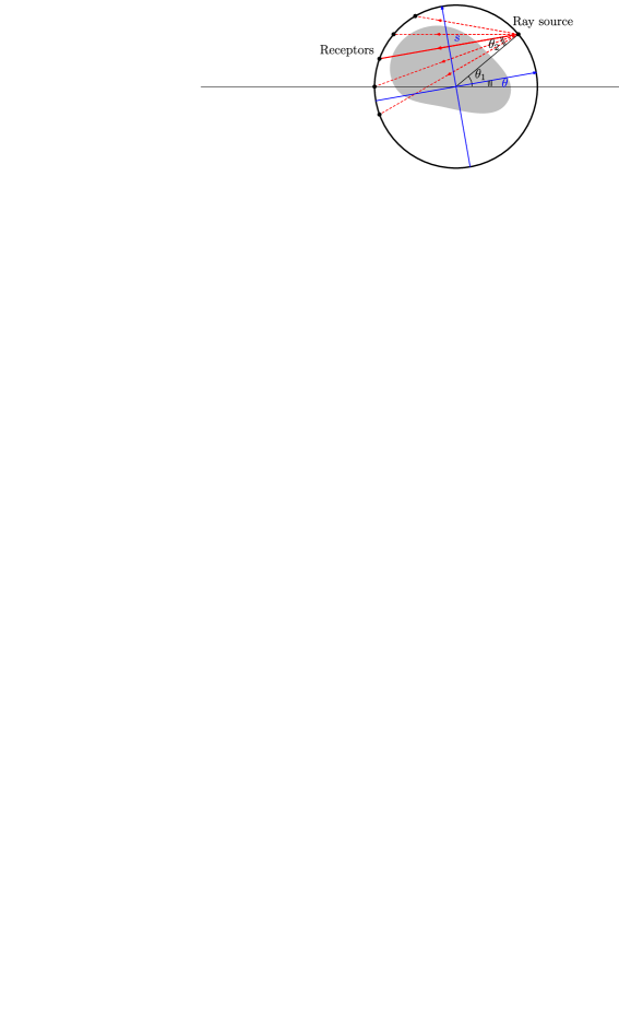
Figure 3: Simplified CAT device.

In our implementation, we exploit the tensorial structure of the SVD basis of the disk in polar coordinates:

$$f_{k,l,m}(r,\theta)=(2k+2)^{1/2}P_{j}^{(0,l)}(2|r|^{2}-1)|r|^{l}Y_{l,m}(\theta),\qquad 0\leq l\leq k,k-l=2j,1\leq m\leq 2,$$

where $P_{j}^{0,l}$ is the corresponding Jacobi polynomial, and $Y_{l,1}(\theta)=c_{l}\cos(l\theta)$ and $Y_{l,2}(\theta)=c_{l}\sin(l\theta)$ with $c_{0}=\frac{1}{\sqrt{2\uppi}}$ and $c_{l}=\frac{1}{\sqrt{\uppi}}$, otherwise. The basis of $S^{2}\times[-1,1]$ has a similar tensorial structure as it is given by

$$g_{k,l,m}(\theta,s)=[h_{k}]^{-1/2}(1-s^{2})^{1/2}C^{1}_{k}(s)Y_{l,m}(\theta),\qquad k\geq 0,l\geq 0,1\leq m\leq 2,$$

where $C^{1}_{k}$ is the Gegenbauer of parameter $1$ and degree $k$. We recall that the corresponding eigenvalues are

$$\lambda_{k}=\frac{2\sqrt{\uppi}}{\sqrt{k+1}}.$$

5.2 SVD, needlet and cubature

In our numerical studies, we compare four different type of estimators: linear SVD estimators, thresholded SVD estimators, linear needlet estimators and thresholded needlet estimators. They are defined from the measurement of the values of the Gaussian field on the SVD basis function $Y_{g_{k,l,m}}$ and the following linear estimates of, respectively, the SVD basis coefficients $\langle f,f_{k,l,m}\rangle$ and the needlet coefficients $\langle f,\psi_{j,\xi}\rangle$,

$$\widehat{\alpha}_{k,l,m}=\frac{1}{\lambda_{k}}Y_{g_{k,l,m}}=\frac{1}{\lambda_{k}}\int g_{k,l,m}\,\mathrm{d}Y$$

and

$$\widehat{\beta}_{j,\xi}=\sqrt{\omega_{j,\xi}}\sum_{k}\sqrt{b(k/2^{j})}\sum_{l,m}g_{k,l,m}(\xi)\widehat{\alpha}_{k,l,m}.$$

The estimators we consider are respectively defined as:

$$\mbox{linear SVD estimates}\hskip 55.0pt\hat{f}^{\mathrm{LS}}_{J}=\sum_{k<2^{J}}\sum_{l,m}\widehat{\alpha}_{k,l,m}f_{k,l,m},$$

$$\mbox{linear needlet estimates}\hskip 44.0pt\hat{f}^{\mathrm{LN}}_{J}=\sum_{j<J}\sum_{\xi}\widehat{\beta}_{j,\xi}\psi_{j,\xi},$$

$$\mbox{thresholded SVD estimates}\hskip 31.0pt\hat{f}^{\mathrm{TS}}_{T}=\sum_{k<2^{J}}\sum_{l,m}\rho_{T_{k}}(\widehat{\alpha}_{k,l,m})f_{k,l,m},$$

$$\mbox{thresholded needlet estimates}\qquad\hat{f}^{\mathrm{TN}}_{T}=\sum_{j<J}\sum_{\xi}\rho_{T_{j,\xi}}(\widehat{\beta}_{j,\xi})\psi_{j,\xi},$$

where $\rho_{T}(\cdot)$ is the hard threshold function with threshold $T$:

$$\rho_{T}(x)=\cases{\displaystyle x,&\quad if $|x|\geq T$,\cr\displaystyle 0,&\quad otherwise.}$$

A more precise description is given in Table 1. In our experiments, the values of $Y_{g_{k,l,m}}$ have been obtained from an initial approximation of $\langle f,f_{k,l,m}\rangle$ computed with a very fine cubature to which a Gaussian i.i.d. sequence is added.

Table 1: Algorithmic description of the considered estimators

	Linear SVD	Thresh. SVD	Linear needlet	Thresh. needlet
	$\hat{f}^{\mathrm{LS}}$	$\hat{f}^{\mathrm{TS}}$	$\hat{f}^{\mathrm{LN}}$	$\hat{f}^{\mathrm{TN}}$
Observation	$\mathrm{d}Y=Rf\,\mathrm{d}\theta\frac{\mathrm{d}s}{\sqrt{1-s^{2}}}+\varepsilon\,\mathrm{d}W$
SVD Dec	$Y_{h_{k,l,}}=\langle Y,g_{k,l,m}\rangle=\langle Rf,g_{k,l,m}\rangle+\varepsilon_{k,l,m}=\mu_{k}\langle f,f_{k,l,m}\rangle+\varepsilon_{k,l,m}$
Inv. Radon	$\widehat{\alpha}_{k,l,m}=\frac{1}{\mu_{k}}\langle Y,g_{k,l,m}\rangle=\langle f,f_{k,l,m}\rangle+\frac{1}{\mu_{k}}\varepsilon_{k,l,m}$
Needlet  transf.			$\widehat{\beta}_{j,\xi}=\sqrt{\omega_{j,\xi}}\sum_{k}\sqrt{b(\frac{k}{2^{j}})}$
			${}\times\sum_{l,m}f_{k,l,m}(\xi)\widehat{\alpha}_{k,l,m}$
Coeff. mod.	$\widehat{\alpha}_{k,l,m}^{SL}=\mathbf{1}_{k\leq k_{\max}}\widehat{\alpha}_{k,l,m}$	$\widehat{\alpha}_{k,l,m}^{ST}=\rho_{T_{k}}(\widehat{\alpha}_{k,l,m})$	$\widehat{\beta}_{j,\xi}^{NL}=\mathbf{1}_{j<j_{\max}}\widehat{\beta}_{j,\xi}$	$\widehat{\beta}_{j,\xi}^{NT}=\rho_{T_{j,\xi}}(\widehat{\beta}_{j,\xi})$
Needlet inv.			$\widehat{\alpha}_{k,l,m}^{\star}=\sum_{j}\sqrt{b(\frac{k}{2^{j}})}$
			${}\times\sum_{\xi\in\chi_{j}}\sqrt{\omega_{j,\xi}}f_{k,l,m}(\xi)\widehat{\beta}_{j,\xi}^{\star}$
SVD rec.	$\hat{f}^{\star}=\sum_{k,l,m}\widehat{\alpha}_{k,l,m}^{\star}f_{k,l,m}$

We have used, in our numerical experiments, thresholds of the form

$$T_{k}=\frac{\kappa}{\lambda_{k}}\varepsilon\sqrt{\log 1/\varepsilon}\quad\mbox{and}\quad T_{j,\xi}=\kappa\sigma_{j,\xi}\varepsilon\sqrt{\log 1/\varepsilon},$$

where $\sigma_{j,\xi}$ is the standard deviation of the noisy needlet coefficients when $f=0$ and $\varepsilon=1$:

$$\sigma_{j,\xi}^{2}=\omega_{j,\xi}\sum_{k}b(k/2^{j})\sum_{l,m}g_{k,l,m}(\xi)^{2}.$$

Note that, while the needlet threshold is different than in Theorem 1, as $\sigma_{j,\xi}$ is of order $2^{j\nu}$, its conclusions remain valid.

An important issue in the needlet scheme is the choice of the cubature in the needlet construction. Proposition 1 ensures the existence of a suitable cubature $\xi_{j}$ for every level $j$ based on a cubature $\widetilde{\xi}_{j}$ on the sphere but gives neither an explicit construction of the points on the sphere nor an explicit formula for the weights $\omega_{j,\xi}$. Those ingredients are, nevertheless, central in the numerical scheme and should be specified.

Three possibilities have been considered: a numerical cubature deduced from an almost uniform cubature of the half sphere available, an approximate cubature deduced from the Healpix cubature on the sphere and a cubature obtained by subsampling a tensorial cubature associated to the latitude and longitude coordinates on the sphere. The first strategy has been considered by Baldi et al. [2] in a slightly different context; there is, however, a strong limitation on the maximum degree of the cubature available and, thus, this solution has been abandoned. The Healpix strategy, also considered by Baldi et al. in another paper [3], is easily implementable but, as it is based on an approximate cubature, fails to be precise enough in our numerical experiments. The last strategy relies on the subsampling on a tensorial grid on the sphere. While such a strategy provides a simple way to construct an admissible cubature, the computation of the cubature weights is becoming an issue as no closed form is available.

To overcome those issues, we have considered a cubature formula based on the full tensorial grid appearing as proposed by [16]. This cubature does not satisfy the condition of Proposition 1, but its weights can be computed explicitly. Furthermore, we argue that, using our modified threshold, we can still control the risk of the estimator. Indeed, note first that the modified threshold is such that the thresholding of a needlet depends only on its scale parameter $j$ and on its center $\xi$ and not on the corresponding cubature weight $\omega_{j,\xi}$. Assume now that we have a collection of $K$ cubature, each satisfying conditions of Proposition 1 and thus defining a suitable estimate, $\hat{f}_{k}$. We can use the “average” cubature obtained by adding all the cubature points and averaging the cubature weights. This new cubature defines a new estimate, $\hat{f}$, satisfying

$$\hat{f}=\frac{1}{K}\sum_{k=1}^{K}\hat{f}_{k}.$$

By convexity, for any $p\geq 1$,

$$\|f-\hat{f}\|_{p}^{p}=\Biggl{\|}f-\frac{1}{K}\sum_{k=1}^{K}\hat{f}_{k}\Biggr{\|}_{p}^{p}\leq\frac{1}{K}\sum_{k=1}^{K}\|f-\hat{f}_{k}\|_{p}^{p}$$

and, thus, this average estimator is as efficient as the worst estimator in the family $\hat{f}_{k}$. The full tensorial cubature is an average of suitable cubatures. The corresponding estimator satisfies the error bounds of Theorems 1 and 2. Note that this principle is quite close to the cycle-spinning method introduced by Donoho et al. Indeed, the same kind of numerical gain is obtained with this method. The numerical comparison of the Healpix cubature and our tensorial cubature is largely in favor of our scheme. Furthermore, as already noticed by [16], the tensorial structure of the cubature leads to some simplification in the numerical implementation of the needlet estimator. The resulting scheme is almost as fast as the Healpix-based one.

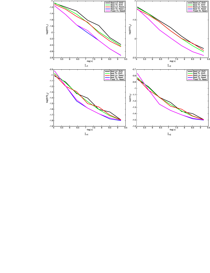
Figure 4: Estimation results in log $\mathbb{L}_{p}$ norm. Each figure shows the decay of the logarithm of the error against the logarithm of the noise parameter for the specified norm.

5.3 Numerical results

In this section, we compare five “estimators” (linear SVD with best scale, linear needlet with best scale, thresholded SVD with best $\kappa$, thresholded needlet with best $\kappa$ and thresholded needlet with $\kappa=3$) for seven different norms ($\mathbb{L}_{1}$, $\mathbb{L}_{2}$, $\mathbb{L}_{4}$, $\mathbb{L}_{6}$, $\mathbb{L}_{7}$, $\mathbb{L}_{8}$, $\mathbb{L}_{10}$ and $\mathbb{L}_{\infty}$) and seven noise levels $\varepsilon$ ($2^{k}/1\,000$ for $k$ in $0,1,\ldots,6$). Each subfigure of Figures 4 and 5 plots the logarithm of the estimation error for a specific norm against the opposite of the logarithm of the noise level. Note that the subfigure overall aspect is explained by the error decay when the noise level diminishes. The good theoretical behavior of the thresholded needlet estimator is confirmed numerically: the thresholded needlet estimator with an optimized $\kappa$ appears as the best estimator for every norm while a fixed $\kappa$ yields a very good estimator, except for the $\mathbb{L}_{\infty}$ case, as expected by our theoretical results. These results are confirmed visually by the reconstructions of Figure 6. In the needlet ones, errors are smaller and much more localized than in their SVD counterparts. Observe also how the fine structures are much more preserved with the thresholded needlet estimate than with any other methods.

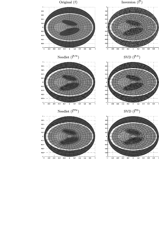
Figure 6: Visual comparison for the original Logan–Shepp phantom with $\varepsilon=8/1\,000$. Errors are much more localized in the needlet-based estimates compared to the fully delocalized errors of the SVD based estimates. Fine structures are much more restored in the thresholded needlet estimate than in the other estimates.

We conclude this paper with some sections devoted to the proofs of our results.

6 Needlet properties

6.1 Key inequalities

The following inequalities are true (and proved in [17, 18, 20, 13]) and will be fundamental in the sequel. In the following lines, $g_{j,\xi}$ will stand either for $\varphi_{j,\xi}$ or $\psi_{j,\xi}$:

$$\displaystyle\forall j\in\mathbb{N},\ \forall\xi\in\chi_{j}\qquad 0<c\leq\|g_{j,\xi}\|_{2}^{2}\leq 1,$$ (14)

$$\displaystyle\forall j\in\mathbb{N},\xi\in\chi_{j},\ \forall x\in{\mathcal{X}}\qquad\sum_{\xi\in\chi_{j}}\|g_{j,\xi}\|_{1}|g_{j,\xi}(x)|\leq C<\infty,$$ (15)

$$\displaystyle|g_{j,\xi}(x)|\leq C_{M}\frac{2^{jd/2}}{\sqrt{W_{j}(x)}(1+2^{j}d(x,\xi))^{M}}$$ (16)

(recall that $W_{j}(x)$ has been defined in (8)). From these inequalities, one can deduce the following ones (see [12]): for all $1\leq p\leq\infty$,

$$\biggl{(}\sum_{\xi\in\chi_{j}}|\langle f,g_{j,\xi}\rangle|^{p}\|g_{j,\xi}\|^{p}_{p}\biggr{)}^{1/p} \leq C\|f\|_{p},$$ (17)

$$\biggl{\|}\sum_{\xi\in\chi_{j}}\lambda_{\xi}g_{j,\xi}(x)\biggr{\|}_{p} \leq \biggl{(}\frac{C}{c}\biggr{)}^{2}\biggl{(}\sum_{\xi\in\chi_{j}}\|\lambda_{\xi}g_{j,\xi}\|^{p}_{p}\biggr{)}^{1/p}.$$ (18)

6.2 Besov embeddings

It is a key point to clarify how the Besov spaces defined above may be included in each of the others. As will be seen, the embeddings will parallel the standard embeddings of usual Besov spaces, but with important differences, which, in particular, yield new minimax rates of convergence as detailed above.

We begin with an evaluation of the different $\mathbb{L}_{p}$ norms of the needlets. More precisely, in [13] it is shown that, for $0<p\leq\infty,$

$$\|\psi_{j,\xi}\|_{p}\sim\|\varphi_{j,\xi}\|_{p}\sim\biggl{(}\frac{2^{jd}}{W_{j}(\xi)}\biggr{)}^{1/2-1/p},\qquad\xi\in\chi_{j}.$$ (19)

The following inequalities are proved in [11]:

$$\sum_{\xi\in\chi_{j}}\|g_{j,\xi}\|^{p}_{p} \leq c2^{j(dp/2+(p/2-2)_{+})}\qquad\mbox{if }p\neq 4,$$ (20)

$$\sum_{\xi\in\chi_{j}}\|g_{j,\xi}\|^{p}_{p} \leq cj2^{jdp/2}\qquad\mbox{if }p=4.$$ (21)

We are now able to state the embedding results (see [12]).

Theorem 4

(1) ${1\leq p\leq\pi\leq\infty\Rightarrow B^{s}_{\pi,r}\subseteq B^{s}_{p,r}}.$

(2) $\infty\geq p\geq\pi>0$, $s>(d+1)(1/\pi-1/p)$, $\Rightarrow B^{s}_{\pi,r}\subseteq B^{s-(d+1)(1/\pi-1/p)}_{p,r}.$

7 Proof of the upper bounds

A important tool for the proof of the upper bounds that clarifies the thresholding procedure is the following lemma.

Lemma 1

For all $j\geq-1$, $\xi\in\chi_{j}$, $\widehat{\beta}_{j,\xi}$ has a Gaussian distribution with mean $\beta_{j,\xi}$ and variance $\sigma^{2}_{j,\xi}$, with

$$\sigma^{2}_{j,\xi}\leq c2^{j(d-1)}\varepsilon^{2}.$$

Proof.

As we can write

$$\widehat{\beta}_{j,\xi} = \sum_{k,l,m}\gamma^{j,\xi}_{k,l,m}\int_{B^{d}}ff_{k,l,m}\,\mathrm{d}x+\sum_{k,l,m}\gamma^{j,\xi}_{k,l,m}\frac{\varepsilon}{\lambda_{k}}Z_{k,l,m}$$

$$= \beta_{j,\xi}+Z_{j,\xi}.$$

Here the summation is over $\{(k,l,m)\colon\ 0\leq k<2^{j},0\leq l\leq k,l\equiv k\ (\operatorname{mod}2),1\leq m\leq N_{d-1}(l)\}$. Since the $Z_{k,l,m}$’s are independent $N(0,1)$ random variables, $Z_{j,\xi}\sim N(0,\sigma^{2}_{j,\xi}),$ we have

$$\sigma^{2}_{j,\xi}=\varepsilon^{2}\sum_{k,l,m}|\gamma^{j,\xi}_{k,l,m}|^{2}\frac{(k)_{d}}{\uppi^{d-1}2^{d}k}\leq\frac{(2^{j})_{d-1}}{\uppi^{d-1}2^{d}}\leq c2^{j(d-1)}\varepsilon^{2}$$ (22)

with $c=(d/2\uppi)^{d-1}$. Here, we used that $\{f_{k,l,m}\}$ is an orthonormal basis for $\mathbb{L}_{2}$ and hence $\sum_{k,l,m}|\gamma^{j,\xi}_{k,l,m}|^{2}=\|\psi_{j,\xi}\|_{2}^{2}\leq 1$. ∎

Let us now begin with the second theorem, the proof of which is slightly simpler.

7.1 Proof of Theorem 2

In this proof, as well as in the other one, $C$ will denote any constant in the sense of Theorems 1–3; we assume that $f$ belongs to the Besov ball $B^{s}_{\pi,r}(M)$ and measure the loss in $\mathbb{L}_{p}$ norm (here, $p=\infty$). Then $C$ denotes a generic quantity that depends only on $s$, $r$, $p$ and $M$. Note that the exact value denoted by $C$ may vary from one line to another.

We have, if we denote

$$A_{J}(f) := \sum_{j>J}\sum_{\xi\in\chi_{j}}{\beta}_{j,\xi}\psi_{j,\xi},$$

$$\|\hat{f}_{\infty}-f\|_{\infty} \leq \|\hat{f}_{\infty}-A_{J}(f)\|_{\infty}+\|A_{J}(f)-f\|_{\infty}$$

$$\leq \|\hat{f}_{\infty}-A_{J}(f)\|_{\infty}+C\|f\|_{B^{s}_{\pi,r}}2^{-J(s-(d+1)/\pi)}.$$

We have used, as $B^{s}_{\pi,r}\subset B^{s-(d+1){1/\pi}}_{\infty,r}$,

$$\|A_{J}f-f\|_{\infty}\leq C\|f\|_{B^{s}_{\pi,r}}2^{-J(s-(d+1){1/\pi})}.$$

Moreover,

$$2^{-J(s-(d+1)/\pi)}\leq\bigl{(}\varepsilon\sqrt{\log 1/\varepsilon}\bigr{)}^{-{(s-(d+1)/\pi)/d}}\leq\bigl{(}\varepsilon\sqrt{\log 1/\varepsilon}\bigr{)}^{-{(s-(d+1)/\pi)/(s-(d+1)/\pi+d)}}$$

as $s>\frac{d+1}{\pi}$.

We have, using (18),

$$\|\hat{f}_{\infty}-A_{J}(f)\|_{\infty} \leq \sum_{j<J}\biggl{\|}\sum_{\xi\in\chi_{j}}\bigl{(}\widehat{\beta}_{j,\xi}1_{\{|\widehat{\beta}_{j,\xi}|\|\psi_{j,\xi}\|_{\infty}\geq\kappa 2^{jd}\varepsilon\sqrt{\log 1/\varepsilon}\}}-{\beta}_{j,\xi}\bigr{)}\psi_{j,\xi}\biggr{\|}_{\infty}$$

$$\leq \sum_{j<J}\biggl{(}\biggl{\|}\sum_{\xi\in\chi_{j}}\bigl{(}(\widehat{\beta}_{j,\xi}-\beta_{j,\xi})\psi_{j,\xi}1_{\{|\widehat{\beta}_{j,\xi}|\|\psi_{j,\xi}\|_{\infty}\geq\kappa 2^{jd}\varepsilon\sqrt{\log 1/\varepsilon}\}}\bigr{)}\biggr{\|}_{\infty}$$

$$\hphantom{\sum_{j<J}\biggl{(}}{}+\biggl{\|}\sum_{\xi\in\chi_{j}}\bigl{(}\beta_{j,\xi}\psi_{j,\xi}1_{\{|\widehat{\beta}_{j,\xi}|\|\psi_{j,\xi}\|_{\infty}<\kappa 2^{jd}\varepsilon\sqrt{\log 1/\varepsilon}\}}\bigr{)}\biggr{\|}_{\infty}\biggr{)}$$

$$\leq \frac{C}{c}\sum_{j<J}\biggl{(}\sup_{\xi\in\chi_{j}}\bigl{(}|\widehat{\beta}_{j,\xi}-\beta_{j,\xi}|\|\psi_{j,\xi}\|_{\infty}1_{\{|\widehat{\beta}_{j,\xi}|\|\psi_{j,\xi}\|_{\infty}\geq\kappa 2^{jd}\varepsilon\sqrt{\log 1/\varepsilon}\}}\bigr{)}$$

$$\hphantom{\frac{C}{c}\sum_{j<J}\biggl{(}}{}+\sup_{\xi\in\chi_{j}}\bigl{(}|\beta_{j,\xi}|\|\psi_{j,\xi}\|_{\infty}1_{\{|\widehat{\beta}_{j,\xi}|\|\psi_{j,\xi}\|_{\infty}<\kappa 2^{jd}\varepsilon\sqrt{\log 1/\varepsilon}\}}\bigr{)}\biggr{)}.$$

We decompose the first term of the last inequality

$$\sup_{\xi\in\chi_{j}}\bigl{(}|\widehat{\beta}_{j,\xi}-\beta_{j,\xi}|\|\psi_{j,\xi}\|_{\infty}1_{\{|\widehat{\beta}_{j,\xi}|\|\psi_{j,\xi}\|_{\infty}\geq\kappa 2^{jd}\varepsilon\sqrt{\log 1/\varepsilon}\}}\bigr{)}$$

$$\quad=\sup_{\xi\in\chi_{j}}\bigl{(}|\widehat{\beta}_{j,\xi}-\beta_{j,\xi}|\|\psi_{j,\xi}\|_{\infty}1_{\{|\widehat{\beta}_{j,\xi}|\|\psi_{j,\xi}\|_{\infty}\geq\kappa 2^{jd}\varepsilon\sqrt{\log 1/\varepsilon}\}}$$

$$\hphantom{\sup_{\xi\in\chi_{j}}\bigl{(}}\qquad{}\times\bigl{(}1_{\{|\beta_{j,\xi}|\|\psi_{j,\xi}\|_{\infty}\geq{(\kappa/2)}2^{jd}\varepsilon\sqrt{\log 1/\varepsilon}\}}+1_{\{|\beta_{j,\xi}|\|\psi_{j,\xi}\|_{\infty}<{(\kappa/2)}2^{jd}\varepsilon\sqrt{\log 1/\varepsilon}\}}\bigr{)}\bigr{)}$$

$$\quad\leq\sup_{\xi\in\chi_{j}}\bigl{(}|\widehat{\beta}_{j,\xi}-\beta_{j,\xi}|\|\psi_{j,\xi}\|_{\infty}1_{\{|\widehat{\beta}_{j,\xi}-\beta_{j,\xi}|\|\psi_{j,\xi}\|_{\infty}\geq{(\kappa/2)}2^{jd}\varepsilon\sqrt{\log 1/\varepsilon}\}}\bigr{)}$$

$$\qquad{}+\sup_{\xi\in\chi_{j}}\bigl{(}|\widehat{\beta}_{j,\xi}-\beta_{j,\xi}|\|\psi_{j,\xi}\|_{\infty}1_{\{|\beta_{j,\xi}|\|\psi_{j,\xi}\|_{\infty}>{(\kappa/2)}2^{jd}\varepsilon\sqrt{\log 1/\varepsilon}\}}\bigr{)}$$

and the second one

$$\sup_{\xi\in\chi_{j}}\bigl{(}|\beta_{j,\xi}|\|\psi_{j,\xi}\|_{\infty}1_{\{|\widehat{\beta}_{j,\xi}|\|\psi_{j,\xi}\|_{\infty}<\kappa 2^{jd}\varepsilon\sqrt{\log 1/\varepsilon}\}}\bigr{)}$$

$$\quad=\sup_{\xi\in\chi_{j}}\bigl{(}|\beta_{j,\xi}|\|\psi_{j,\xi}\|_{\infty}1_{\{|\widehat{\beta}_{j,\xi}|\|\psi_{j,\xi}\|_{\infty}<\kappa 2^{jd}\varepsilon\sqrt{\log 1/\varepsilon}\}}$$

$$\hphantom{\sup_{\xi\in\chi_{j}}\bigl{(}}\qquad{}\times\bigl{(}1_{\{|\beta_{j,\xi}|\|\psi_{j,\xi}\|_{\infty}\geq 2\kappa 2^{jd}\varepsilon\sqrt{\log 1/\varepsilon}\}}+1_{\{|\beta_{j,\xi}|\|\psi_{j,\xi}\|_{\infty}<\kappa 2^{jd}\varepsilon\sqrt{\log 1/\varepsilon}\}}\bigr{)}\bigr{)}$$

$$\quad\leq\sup_{\xi\in\chi_{j}}\bigl{(}|\beta_{j,\xi}|\|\psi_{j,\xi}\|_{\infty}1_{\{|\widehat{\beta}_{j,\xi}-\beta_{j,\xi}|\|\psi_{j,\xi}\|_{\infty}>\kappa 2^{jd}\varepsilon\sqrt{\log 1/\varepsilon}\}}\bigr{)}$$

$$\qquad{}+\sup_{\xi\in\chi_{j}}\bigl{(}|\beta_{j,\xi}|\|\psi_{j,\xi}\|_{\infty}1_{\{|\beta_{j,\xi}|\|\psi_{j,\xi}\|_{\infty}<\kappa 2^{jd}\varepsilon\sqrt{\log 1/\varepsilon}\}}\bigr{)}.$$

Now we will bound each of the four terms coming from the last two inequalities. Since for $X\sim N(0,\sigma^{2}),$ we have

$$\mathbb{E}\bigl{(}|Y|1_{\{|Y|>\lambda\sigma\}}\bigr{)}=\sigma\frac{2}{\sqrt{2\uppi}}\int_{\lambda}^{\infty}y\mathrm{e}^{-y^{2}/2}\,\mathrm{d}y=\mathrm{e}^{-\lambda^{2}/2}\frac{2}{\sqrt{2\uppi}}\leq\mathrm{e}^{-\lambda^{2}/2}.$$

Noticing that the standard deviation of $(\widehat{\beta}_{j,\xi}-\beta_{j,\xi})\|\psi_{j,\xi}\|_{\infty}$ is smaller than $\tau_{\infty}2^{jd}\varepsilon$ (using Lemma 1 and (16)), we have

$$\sum_{j\leq J}\mathbb{E}\biggl{(}\sup_{\xi\in\chi_{j}}\bigl{(}|\widehat{\beta}_{j,\xi}-\beta_{j,\xi}|\|\psi_{j,\xi}\|_{\infty}1_{\{|\widehat{\beta}_{j,\xi}-\beta_{j,\xi}|\|\psi_{j,\xi}\|_{\infty}\geq{(\kappa/2)}2^{jd}\varepsilon\sqrt{\log 1/\varepsilon}\}}\bigr{)}\biggr{)}$$

$$\quad\leq\sum_{j\leq J}\sum_{\xi\in\chi_{j}}\mathbb{E}\bigl{(}|\widehat{\beta}_{j,\xi}-\beta_{j,\xi}|\|\psi_{j,\xi}\|_{\infty}1_{\{|\widehat{\beta}_{j,\xi}-\beta_{j,\xi}|\|\psi_{j,\xi}\|_{\infty}\geq{(\kappa/2)}2^{jd}\varepsilon\sqrt{\log 1/\varepsilon}\}}\bigr{)}\leq c2^{Jd}\varepsilon^{\kappa^{2}/2\tau_{\infty}^{2}}$$

$$\quad\leq C\varepsilon^{\kappa^{2}/2\tau_{\infty}^{2}-1}\sqrt{\log 1/\varepsilon}^{-1}\leq C\varepsilon\sqrt{\log 1/\varepsilon}$$

if $\kappa^{2}\geq 4\tau_{\infty}^{2},$ where we have used $\operatorname{Card}{\chi_{j}}\leq c2^{jd}$. This proves that this term will be of the right order.

For the second term, let us observe that we have, using Theorem 4,

$$|\beta_{j,\xi}|\|\psi_{j,\xi}\|_{\infty}\leq C\|f\|_{B^{s}_{\pi,r}}2^{-j(s-(d+1)/\pi)},$$

so only the $j$’s index such that $j\leq j_{1}$ will verify this inequality:

$$2^{j_{1}}\sim\biggl{(}\frac{2C\|f\|_{B^{s}_{\pi,r}}}{\kappa}\bigl{(}\varepsilon\sqrt{\log 1/\varepsilon}\bigr{)}\biggr{)}^{-{1/(s+d-(d+1)\pi)}}.$$

On the other side, using the Pisier lemma [23],

$$\mathbb{E}\biggl{(}\sup_{\xi\in\chi_{j}}(|\widehat{\beta}_{j,\xi}-\beta_{j,\xi}|\|\psi_{j,\xi}\|_{\infty})\biggr{)}\leq\tau_{\infty}2^{jd}\varepsilon\sqrt{2\log{2c2^{jd}}}.$$

So

$$\sum_{j\leq j_{1}}\mathbb{E}\Bigl{(}\sup_{\xi\in\chi_{j}}\bigl{(}|\widehat{\beta}_{j,\xi}-\beta_{j,\xi}|\|\psi_{j,\xi}\|_{\infty}1_{\{|\beta_{j,\xi}|\|\psi_{j,\xi}\|_{\infty}>{(\kappa/2)}2^{jd}\varepsilon\sqrt{\log 1/\varepsilon}\}}\bigr{)}\Bigr{)}$$

$$\quad\leq\tau_{\infty}\sum_{j\leq j_{1}}2^{jd}\varepsilon\sqrt{2\log{2c2^{jd}}}\leq C\varepsilon j_{1}^{{1/2}}2^{j_{1}d}$$

$$\quad\lesssim C(\|f\|_{B^{s}_{\pi,r}})^{{(s-(d+1)\pi)/(s+d-(d+1)/\pi)}}\bigl{(}\varepsilon\sqrt{\log 1/\varepsilon}\bigr{)}^{{(s-(d+1)/\pi)/(s+d-(d+1)/\pi)}}.$$

This proves that this term will be of the right order. Concerning the first term of the second inequality,

$$\mathbb{E}\Bigl{(}\sup_{\xi\in\chi_{j}}\bigl{(}|\beta_{j,\xi}|\|\psi_{j,\xi}\|_{\infty}1_{\{|\widehat{\beta}_{j,\xi}-\beta_{j,\xi}|\|\psi_{j,\xi}\|_{\infty}>\kappa 2^{jd}\varepsilon\sqrt{\log 1/\varepsilon}\}}\bigr{)}\Bigr{)}$$

$$\quad\leq C\|f\|_{B^{s}_{\pi,r}}\sum_{\xi\in\chi_{j}}P\bigl{(}|\widehat{\beta}_{j,\xi}-\beta_{j,\xi}|\|\psi_{j,\xi}\|_{\infty}>\kappa 2^{jd}\varepsilon\sqrt{\log 1/\varepsilon}\bigr{)}$$

but

$$P\bigl{(}|\widehat{\beta}_{j,\xi}-\beta_{j,\xi}|\|\psi_{j,\xi}\|_{\infty}>\kappa 2^{jd}\varepsilon\log 1/\varepsilon\bigr{)}\leq\mathrm{e}^{-{(\kappa 2^{jd}\varepsilon\sqrt{\log 1/\varepsilon})^{2}/(2(\varepsilon 2^{j(d-1)/2}\|\psi_{j,\xi}\|_{\infty})^{2})}}\leq\varepsilon^{\kappa^{2}/2\tau_{\infty}^{2}}.$$

So

$$\sum_{j\leq J}\mathbb{E}\biggl{(}\sup_{\xi\in\chi_{j}}\bigl{(}|\beta_{j,\xi}|\|\psi_{j,\xi}\|_{\infty}1_{\{|\widehat{\beta}_{j,\xi}-\beta_{j,\xi}|\|\psi_{j,\xi}\|_{\infty}>\kappa 2^{jd}\varepsilon\sqrt{\log 1/\varepsilon}\}}\bigr{)}\biggr{)}$$

$$\quad\leq C\|f\|_{B^{s}_{\pi,r}}J\varepsilon^{\kappa^{2}/2\tau_{\infty}^{2}}\leq C\|f\|_{B^{s}_{\pi,r}}\bigl{(}\varepsilon\sqrt{\log 1/\varepsilon}\bigr{)}^{{(s-(d+1)/\pi)/(s+d-(d+1)/\pi)}}$$

if $\kappa^{2}/2\geq\tau_{\infty}^{2}.$ This proves that this term will be of the right order. Concerning the second term of the second inequality,

$$\sup_{\xi\in\chi_{j}}\bigl{(}|\beta_{j,\xi}|\|\psi_{j,\xi}\|_{\infty}1_{\{|\beta_{j,\xi}|\|\psi_{j,\xi}\|_{\infty}<2\kappa 2^{jd}\varepsilon\sqrt{\log 1/\varepsilon}\}}\bigr{)}$$

$$\quad\leq 2\kappa 2^{jd}\varepsilon\sqrt{\log 1/\varepsilon}\wedge C\|f\|_{B^{s}_{\pi,r}}2^{-j(s-(d+1)/\pi)},$$

let us again take

$$2^{j_{1}}\sim\bigl{(}\varepsilon\sqrt{\log 1/\varepsilon}\bigr{)}^{-{1/(s+d-(d+1)\pi)}}$$

$$\sum_{j\leq J}\sup_{\xi\in\chi_{j}}\bigl{(}|\beta_{j,\xi}|\|\psi_{j,\xi}\|_{\infty}1_{\{|\beta_{j,\xi}|\|\psi_{j,\xi}\|_{\infty}<2\kappa 2^{jd}\varepsilon\log 1/\varepsilon\}}\bigr{)}$$

$$\quad\leq C\|f\|_{B^{s}_{\pi,r}}\biggl{(}\varepsilon\log 1/\varepsilon\sum_{j\leq j_{1}}2^{jd}+\sum_{j_{1}<j\leq J}2^{-j(s-(d+1)/\pi)}\biggr{)}$$

$$\quad\lesssim C\|f\|_{B^{s}_{\pi,r}}\bigl{(}\varepsilon\sqrt{\log 1/\varepsilon}\bigr{)}^{{(s-(d+1)/\pi)/(s+d-(d+1)/\pi)}}.$$

This ends the proof of Theorem 2.

7.2 Proof of Theorem 1

As in the previous proof, we begin with the decomposition,

$$\|\hat{f_{\varepsilon}}-f\|^{p}_{p}\leq 2^{p-1}\bigl{(}\|\hat{f_{\varepsilon}}-A_{J}(f)\|^{p}_{p}+\|A_{J}(f)-f\|^{p}_{p}\bigr{)}.$$

Using the fact that, for $\pi\geq p$, $B^{s}_{\pi,r}\subset B^{s}_{p,\infty},$ and for $\pi\leq p,B^{s}_{\pi,r}\subset B^{s-(d+1)(1/\pi-1/p)}_{p,\infty}$, we obtain

$$\|A_{J}(f)-f\|_{p}^{p}\leq C\|f\|^{p}_{B^{s}_{\pi,r}}2^{-Jsp}\qquad\mbox{if }\pi\geq p$$

and

$$\|A_{J}(f)-f\|_{p}^{p}\leq C\|f\|^{p}_{B^{s}_{\pi,r}}2^{-J(s-(d+1)(1/\pi-1/p))p}\qquad\mbox{if }\pi\leq p.$$

We have $2^{-Jsp}\leq(\varepsilon\sqrt{\log 1/\varepsilon})^{{sp/(d-{1/2})}}\leq(\varepsilon\sqrt{\log 1/\varepsilon})^{{sp/(s+d-{1/2})}}$. Obviously, this term has the right rate for $\pi\geq p$. For $\pi<p$,

$$2^{-J(s-(d+1)(1/\pi-1/p))} \leq (\varepsilon\log 1/\varepsilon)^{{(s-(d+1)(1/\pi-1/p))/(d-{1/2})}}$$

$$\leq (\varepsilon\log 1/\varepsilon)^{{(s-(d+1)(1/\pi-1/p))/(s+d-(d+1)/\pi)}},$$

thanks to $s\geq(d+1)/\pi-1/2$. This gives the right rate for $dp>d+1.$ For $dp\leq d+1$, we have (again as $s\geq(d+1)/\pi-1/2$ ), $s-(d+1)(\frac{1}{\pi}-\frac{1}{p})\geq d-\frac{1}{2}$, so $2^{-J(s-(d+1)(1/\pi-1/p))}\leq(\varepsilon\log 1/\varepsilon)^{{(s-(d+1)(1/\pi-1/p))/(d-{1/2})}}\leq(\varepsilon\log 1/\varepsilon)^{{s/(s+d-{1/2})}}$. Finally, this proves that the bias term above always has the right rate.

Let us now investigate the stochastic term

$$\mathbb{E}\|\hat{f}-A_{J}(f)\|^{p}_{p}\leq CJ^{p-1}\sum_{j<J}\mathbb{E}\biggl{\|}\sum_{\xi\in\chi_{j}}\bigl{(}\widehat{\beta}_{j,\xi}1_{\{|\widehat{\beta}_{j,\xi}|\geq\kappa 2^{j\nu}\varepsilon\sqrt{\log 1/\varepsilon}\}}-\beta_{j,\xi}\bigr{)}\psi_{j,\xi}\biggr{\|}^{p}_{p}.$$

But

$$\biggl{\|}\sum_{\xi\in\chi_{j}}\bigl{(}\widehat{\beta}_{j,\xi}1_{\{|\widehat{\beta}_{j,\xi}|\geq\kappa 2^{j\nu}\varepsilon\sqrt{\log 1/\varepsilon}\}}-\beta_{j,\xi}\bigr{)}\psi_{j,\xi}\biggr{\|}^{p}_{p}$$

$$\quad\leq C2^{p-1}\biggl{(}\biggl{\|}\sum_{\xi\in\chi_{j}}\bigl{(}(\widehat{\beta}_{j,\xi}-\beta_{j,\xi})\psi_{j,\xi}1_{\{|\widehat{\beta}_{j,\xi}|\geq\kappa 2^{j\nu}\varepsilon\sqrt{\log 1/\varepsilon}\}}\bigr{)}\biggr{\|}^{p}_{p}$$

$$\hphantom{C2^{p-1}\biggl{(}}\qquad{}+\biggl{\|}\sum_{\xi\in\chi_{j}}\bigl{(}\beta_{j,\xi}\psi_{j,\xi}1_{\{|\widehat{\beta}_{j,\xi}|<\kappa 2^{j\nu}\varepsilon\sqrt{\log 1/\varepsilon}\}}\bigr{)}\biggr{\|}^{p}_{p}\biggr{)}$$

$$\quad\leq C\biggl{(}\sum_{\xi\in\chi_{j}}|\widehat{\beta}_{j,\xi}-\beta_{j,\xi}|^{p}\|\psi_{j,\xi}\|^{p}_{p}1_{\{|\widehat{\beta}_{j,\xi}|\geq\kappa 2^{j\nu}\varepsilon\sqrt{\log 1/\varepsilon}\}}$$

$$\hphantom{C\biggl{(}}\qquad{}+\sum_{\xi\in\chi_{j}}|\beta_{j,\xi}|^{p}\|\psi_{j,\xi}\|^{p}_{p}1_{\{|\widehat{\beta}_{j,\xi}<\kappa 2^{j\nu}\varepsilon\sqrt{\log 1/\varepsilon}\}}\biggr{)}.$$

In turn,

$$|\widehat{\beta}_{j,\xi}-\beta_{j,\xi}|^{p}1_{\{|\widehat{\beta}_{j,\xi}|\geq\kappa 2^{j\nu}\varepsilon\sqrt{\log 1/\varepsilon}\}}$$

$$\quad=|\widehat{\beta}_{j,\xi}-\beta_{j,\xi}|^{p}1_{\{|\widehat{\beta}_{j,\xi}|\geq\kappa 2^{j\nu}\varepsilon\sqrt{\log 1/\varepsilon}\}}\bigl{(}1_{\{|\beta_{j,\xi}|\geq{(\kappa/2)}2^{j\nu}\varepsilon\sqrt{\log 1/\varepsilon}\}}+1_{\{\beta_{j,\xi}|<{(\kappa/2)}2^{j\nu}\varepsilon\sqrt{\log 1/\varepsilon}\}}\bigr{)}$$

$$\quad\leq|\widehat{\beta}_{j,\xi}-\beta_{j,\xi}|^{p}1_{\{|\widehat{\beta}_{j,\xi}-\beta_{j,\xi}|\geq{(\kappa/2)}2^{j\nu}\varepsilon\sqrt{\log 1/\varepsilon}\}}+|\widehat{\beta}_{j,\xi}-\beta_{j,\xi}|^{p}1_{\{|\beta_{j,\xi}|>{(\kappa/2)}2^{jd}\varepsilon\sqrt{\log 1/\varepsilon}\}}$$

and

$$|\beta_{j,\xi}|^{p}1_{\{|\widehat{\beta}_{j,\xi}<\kappa 2^{jd}\varepsilon\sqrt{\log 1/\varepsilon}\}} = |\beta_{j,\xi}|^{p}1_{\{|\widehat{\beta}_{j,\xi}<\kappa 2^{jd}\varepsilon\sqrt{\log 1/\varepsilon}\}}$$

$${}\times\bigl{(}1_{\{|\beta_{j,\xi}|\geq 2\kappa 2^{jd}\varepsilon\sqrt{\log 1/\varepsilon}\}}+1_{\{|\beta_{j,\xi}|<\kappa 2^{jd}\varepsilon\sqrt{\log 1/\varepsilon}\}}\bigr{)}$$

$$\leq |\beta_{j,\xi}|^{p}1_{\{|\widehat{\beta}_{j,\xi}-\beta_{j,\xi}|>\kappa 2^{jd}\varepsilon\sqrt{\log 1/\varepsilon}\}}+|\beta_{j,\xi}|^{p}1_{\{|\beta_{j,\xi}|<\kappa 2^{jd}\varepsilon\sqrt{\log 1/\varepsilon}\}}.$$

We now have the following bound using direct computation:

$$\mathbb{E}\bigl{(}|\widehat{\beta}_{j,\xi}-\beta_{j,\xi}|^{p}1_{\{|\widehat{\beta}_{j,\xi}-\beta_{j,\xi}|\geq{(\kappa/2)}2^{j\nu}\varepsilon\sqrt{\log 1/\varepsilon}\}}\bigr{)}\leq C2^{jp\nu}\varepsilon^{p}\bigl{(}\kappa\sqrt{\log 1/\varepsilon}\bigr{)}^{p-1}\varepsilon^{\kappa^{2}/2}.$$

Hence,

$$J^{p-1}\sum_{j\leq J}\sum_{\xi\in\chi_{j}}\mathbb{E}\bigl{(}|\widehat{\beta}_{j,\xi}-\beta_{j,\xi}|^{p}\|\psi_{j,\xi}\|_{p}^{p}1_{\{|\widehat{\beta}_{j,\xi}-\beta_{j,\xi}|\geq{(\kappa/2)}2^{j\nu}\varepsilon\sqrt{\log 1/\varepsilon}\}}\bigr{)}$$

$$\quad\leq CJ^{p-1}\sum_{j\leq J}\varepsilon^{p}\bigl{(}\kappa\sqrt{\log 1/\varepsilon}\bigr{)}^{p-1}\varepsilon^{\kappa^{2}/2}\sum_{\xi\in\chi_{j}}\|\psi_{j,\xi}\|_{p}^{p}$$

$$\quad\leq C\sqrt{\log 1/\varepsilon}^{p-1}\varepsilon^{p}\bigl{(}\kappa\sqrt{\log 1/\varepsilon}\bigr{)}^{p-1}\varepsilon^{\kappa^{2}/2}\sum_{j\leq J}2^{jp\nu}2^{j(dp/2+(p/2-2)_{+})}$$

$$\quad\leq C\varepsilon^{p}$$

if $\kappa\geq\sqrt{2p}$ is large enough (we have used (19)).

Using the forthcoming inequality (24),

$$\sum_{\xi\in\chi_{j}}\mathbb{E}\bigl{(}|\widehat{\beta}_{j,\xi}-\beta_{j,\xi}|^{p}\|\psi_{j,\xi}\|_{p}^{p}1_{\{|\beta_{j,\xi}|>{(\kappa/2)}2^{j\nu}\varepsilon\sqrt{\log 1/\varepsilon}\}}\bigr{)}$$

$$\quad\leq C\varepsilon^{p}\sum_{\xi\in\chi_{j}}2^{j\nu p}\|\psi_{j,\xi}\|_{p}^{p}1_{\{|\beta_{j,\xi}|>{(\kappa/2)}2^{j\nu}\varepsilon\sqrt{\log 1/\varepsilon}\}}$$

$$\quad\leq C\varepsilon^{p}\biggl{(}\frac{\kappa}{2}\varepsilon\sqrt{\log 1/\varepsilon}\biggr{)}^{-q}.$$

Hence,

$$J^{p-1}\sum_{j\leq J}\sum_{\xi\in\chi_{j}}\mathbb{E}\bigl{(}|\widehat{\beta}_{j,\xi}-\beta_{j,\xi}|^{p}\|\psi_{j,\xi}\|_{p}^{p}1_{\{|\beta_{j,\xi}|>{(\kappa/2)}2^{j\nu}\varepsilon\sqrt{\log 1/\varepsilon}\}}\bigr{)}$$

$$\quad\leq CJ^{p}\sqrt{\log 1/\varepsilon}^{-p}\biggl{(}\frac{\kappa}{2}\biggr{)}^{-q}\bigl{(}\varepsilon\sqrt{\log 1/\varepsilon}\bigr{)}^{p-q}$$

and, as $J\leq\frac{1}{d-1/2}\log 1/\varepsilon+1$,

$$\leq C\bigl{(}\varepsilon\sqrt{\log 1/\varepsilon}\bigr{)}^{p-q}(\log 1/\varepsilon)^{p/2}.$$

This term is thus of the right rate. Let us now turn to

$$\sum_{\xi\in\chi_{j}}\mathbb{E}\bigl{(}|\beta_{j,\xi}|^{p}\|\psi_{j,\xi}\|_{p}^{p}1_{\{|\widehat{\beta}_{j,\xi}-\beta_{j,\xi}|>\kappa 2^{j\nu}\varepsilon\sqrt{\log 1/\varepsilon}\}}\bigr{)}$$

$$\quad=\sum_{\xi\in\chi_{j}}|\beta_{j,\xi}|^{p}\|\psi_{j,\xi}\|_{p}^{p}P\bigl{(}|\widehat{\beta}_{j,\xi}-\beta_{j,\xi}|>\kappa 2^{j\nu}\varepsilon\sqrt{\log 1/\varepsilon}\bigr{)}.$$

As the standard deviation of $\widehat{\beta}_{j,\xi}-\beta_{j,\xi}$ is smaller than $\varepsilon 2^{j(d-1)/2}$,

$$P\bigl{(}|\widehat{\beta}_{j,\xi}-\beta_{j,\xi}|>\kappa 2^{j\nu}\varepsilon\sqrt{\log 1/\varepsilon}\bigr{)}\leq\varepsilon^{\kappa^{2}/2}.$$

So

$$J^{p-1}\sum_{j\leq J}\mathbb{E}\biggl{(}\sum_{\xi\in\chi_{j}}|\beta_{j,\xi}|^{p}\|\psi_{j,\xi}\|_{p}^{p}1_{\{|\widehat{\beta}_{j,\xi}-\beta_{j,\xi}|>\kappa 2^{j\nu}\varepsilon\sqrt{\log 1/\varepsilon}\}}\biggr{)}$$

$$\quad\leq C\|f\|_{B^{s}_{\pi,r}}^{p}J^{p-1}\varepsilon^{\kappa^{2}/2}\leq C\bigl{(}\varepsilon\sqrt{\log 1/\varepsilon}\bigr{)}^{p}$$

if $\kappa^{2}$ is large enough (where we have used that $B^{s}_{\pi,r}\subset B^{s^{\prime}}_{p,r}\subset\mathbb{L}_{p}$ with $s^{\prime}=s-(d+1)(1/\pi-1/p)$). Hence this term also is of the right order.

Let us turn now to the last one, using (24)

$$\sum_{\xi\in\chi_{j}}|\beta_{j,\xi}|^{p}\|\psi_{j,\xi}\|_{p}^{p}1_{\{|\beta_{j,\xi}|<2\kappa 2^{j\nu}\varepsilon\sqrt{\log 1/\varepsilon}\}}\leq\bigl{(}2\kappa\varepsilon\sqrt{\log 1/\varepsilon}\bigr{)}^{p-q}.$$

Hence,

$$J^{p-1}\sum_{j\leq J}\sup_{\xi\in\chi_{j}}\bigl{(}|\beta_{j,\xi}|\|^{p}\psi_{j,\xi}\|_{p}^{p}1_{\{|\beta_{j,\xi}|<2\kappa 2^{j\nu}\varepsilon\sqrt{\log 1/\varepsilon}\}}\bigr{)}$$

$$\quad\leq C\|f\|_{B^{s}_{\pi,r}}J^{p}\bigl{(}\varepsilon\sqrt{\log 1/\varepsilon}\bigr{)}^{p-q}\leq C\|f\|_{B^{s}_{\pi,r}}\sqrt{\log 1/\varepsilon}^{p}\bigl{(}\varepsilon\sqrt{\log 1/\varepsilon}\bigr{)}^{p-q}.$$

This proves that all the terms have the proper rate. It remains now to state and prove the following lemma.

Lemma 2

Let $A=\{(s,\pi),s>(d+1)(\frac{1}{\pi}-\frac{1}{p})\cap(s>0)\},$ and $f\in B^{s}_{\pi,r},1\leq\pi\leq\infty,1\leq p<\infty.$ If $\sum_{\xi\in\chi_{j}}(|\beta_{j,\xi}|\|\psi_{j,\xi}\|_{\pi})^{\pi}=\rho_{j}^{\pi}2^{-js\pi}$ with $\rho\in l_{r}(\mathbb{N})$, then, with $\nu=\frac{d-1}{2}$,

$$\sum_{\xi\in\chi_{j}}\biggl{(}\frac{|\beta_{j,\xi}|}{2^{j\nu}}\biggr{)}^{q}(2^{j\nu}\|\psi_{j,\xi}\|_{p})^{p}\leq C\rho_{j}^{q},$$

where $q<p$ is as follows: (

• 3)]

• $p-q=\frac{sp}{s+d-1/2}(q=\frac{(d-1/2)p}{s+d-1/2})$ in the following domain I:

  $$\bigl{\{}(s,\pi),\bigl{(}s(1/p-1/4)\geq(d-1/2)(1/\pi-1/p)\bigr{)}\cap A\bigr{\}}.$$

  Moreover, we have the following slight modification at the frontier: the domain becomes

  $$\bigl{\{}(s,\pi),\bigl{(}s(1/p-1/4)=(d-1/2)(1/\pi-1/p)\bigr{)}\cap A\bigr{\}}$$

  and the inequality

  $$\sum_{\xi\in\chi_{j}}\biggl{(}\frac{|\beta_{j,\xi}|}{2^{j\nu}}\biggr{)}^{q}(2^{j\nu}\|\psi_{j,\xi}\|_{p})^{p}\leq C\rho_{j}^{q}j^{1-q/\pi}.$$

• $p-q=\frac{(s-2(1/\pi-1/p))p}{s+d-2/\pi}$ $(q=\frac{dp+2}{s+d-2/\pi})$ in the following domain II:

  $$\bigl{\{}(s,\pi)\bigl{(}s>dp(1/\pi-1/p)\bigr{)}\cap\bigl{(}s(1/p-1/4)<(d-1/2)(1/\pi-1/p)\bigr{)}\cap A\bigr{\}}.$$

• $p-q=\frac{(s-(d+1)(1/\pi-1/p))p}{s+d-(d+1)/\pi}$ $(q=\frac{dp-(d+1)}{s+d-(d+1)/\pi})$ in the following domain III:

  $$\biggl{\{}(s,\pi),\biggl{(}dp\biggl{(}\frac{1}{\pi}-\frac{1}{p}\biggr{)}\geq s\biggr{)}\cap A,\mbox{ for }\frac{1}{p}<\frac{d}{d+1}\biggr{\}}.$$

This lemma is to be used essentially through the following corollary.

Corollary 1

Respectively, in the domains I, II, III, we have, for $q$ described in the lemma and $f\in B^{s}_{\pi,r}$,

$$\sum_{\xi\in\chi_{j}}1_{\{{|\beta_{j,\xi}|/2^{j\nu}}\geq\lambda\}}(2^{j\nu}\|\psi_{j,\xi}\|_{p})^{p}\leq C\rho_{j}^{q}\lambda^{-q},$$ (23)

$$\sum_{\xi\in\chi_{j}}1_{\{{|\beta_{j,\xi}|/2^{j\nu}}\leq 2^{j\nu}\lambda\}}|\beta_{j,\xi}|^{p}\|\psi_{j,\xi}\|_{p}^{p}\leq C\rho_{j}^{q}\lambda^{p-q}$$ (24)

with an obvious modification for

$$\bigl{\{}(s,\pi),\bigl{(}s(1/p-1/4)=(d-1/2)(1/\pi-1/p)\bigr{)}\cap A\bigr{\}}.$$

Proof.

Let us recall that on a measure space $(X,\mu)$ we have, if $h\in\mathbb{L}_{q}(\mu)$ then $\mu(|h|\geq\lambda)\leq\frac{\|h\|_{q}^{q}}{\lambda^{q}}$ and, as $q<p,$

$$\int_{|h|\leq\lambda}|h|^{p}\,\mathrm{d}\mu \leq \int(|h|\wedge\lambda)^{p}\,\mathrm{d}\mu=\int_{0}^{\lambda}px^{p-1}\mu(|h|\geq x)\,\mathrm{d}x$$

$$\leq \int_{0}^{\lambda}px^{p-1}\frac{\|h\|_{q}^{q}}{x^{q}}\,\mathrm{d}x=\frac{p\|h\|_{q}^{q}}{p-q}\lambda^{p-q}.$$

For the corollary, we take $X=\chi_{j}$, $\mu(\xi)=(2^{j\nu}\|\psi_{j,\xi}\|_{p})^{p}$ and $h(\xi)=\frac{|\beta_{j,\xi}|}{2^{j\nu}}.$ ∎

Proof of Lemma 2 Let us fix $q$ (chosen later) and investigate separately the two cases $q\geq\pi$ and $q<\pi.$

For $q\geq\pi$, we have, using (19),

$$I_{j}(f,q,p) = \sum_{\xi\in\chi_{j}}\biggl{|}\frac{\beta_{j,\xi}}{2^{j\nu}}\biggr{|}^{q}\|2^{j\nu}\psi_{j,\xi}\|_{p}^{p}\sim 2^{j\nu(p-q)}\sum_{\xi\in\chi_{j}}|\beta_{j,\xi}|^{q}\biggl{(}\frac{2^{jd}}{W_{j}(\xi)}\biggr{)}^{p/2-1}$$

$$\leq 2^{j\nu(p-q)}\biggl{(}\sum_{\xi\in\chi_{j}}\biggl{(}|\beta_{j,\xi}|^{q}\biggl{(}\frac{2^{jd}}{W_{j}(\xi)}\biggr{)}^{p/2-1}\biggr{)}^{\pi/q}\biggr{)}^{q/\pi}$$

$$= 2^{j\nu(p-q)}\biggl{(}\sum_{\xi\in\chi_{j}}|\beta_{j,\xi}|^{\pi}\biggl{(}\frac{2^{jd}}{W_{j}(\xi)}\biggr{)}^{(p/2-1)\pi/q}\biggr{)}^{q/\pi}$$

$$= 2^{j\nu(p-q)}\biggl{(}\sum_{\xi\in\chi_{j}}|\beta_{j,\xi}|^{\pi}\biggl{(}\frac{2^{jd}}{W_{j}(\xi)}\biggr{)}^{\pi/2-1}\biggl{(}\frac{2^{jd}}{W_{j}(\xi)}\biggr{)}^{{(\pi/q)}(p/2-1)-(\pi/2-1)}\biggr{)}^{q/\pi}$$

$$\leq 2^{j\nu(p-q)}\biggl{(}\sum_{\xi\in\chi_{j}}|\beta_{j,\xi}|^{\pi}\biggl{(}\frac{2^{jd}}{W_{j}(\xi)}\biggr{)}^{\pi/2-1}\biggr{)}^{q/\pi}2^{j(d+1)({(p-q)/2}+q({1/\pi}-{1/q})}$$

if we choose $q$ such that $(sq+d(p-q)+(d+1)q(\frac{1}{\pi}-\frac{1}{q}))=0$ gives $q=\frac{pd-(d+1)}{s+d-(d+1)\pi}$. Hence, $p-q=\frac{s-(d+1)(1/\pi-1/p)}{s+d-(d+1)\pi}p$; $q-\pi=-\pi\frac{s-pd(1/\pi-1/p)}{s+d-(d+1)\pi}.$ Thus, in domain III,

$$\biggl{\{}\biggl{(}\frac{1}{p}<\frac{d}{d+1}\biggr{)}\cap\bigl{(}s-(d+1)(1/\pi-1/p)>0\bigr{)}\cap\bigl{(}s-pd(1/\pi-1/p)\leq 0\bigr{)}\biggr{\}},$$

we have $0<q<p$, $\pi\leq q$, $\sum_{\xi\in\chi_{j}}|\frac{\beta_{j,\xi}}{2^{j\nu}}|^{q}\|2^{j\nu}\psi_{j,\xi}\|_{p}^{p}\leq\rho_{j}^{q}$.

For $q<\pi$, we have, using (19),

$$I_{j}(f,q,p)=\sum_{\xi\in\chi_{j}}\biggl{|}\frac{\beta_{j,\xi}}{2^{j\nu}}\biggr{|}^{q}\|2^{j\nu}\psi_{j,\xi}\|_{p}^{p}\sim 2^{j\nu(p-q)}\sum_{\xi\in\chi_{j}}|\beta_{j,\xi}|^{q}\biggl{(}\frac{2^{jd}}{W_{j}(\xi)}\biggr{)}^{p/2-1},$$

$$2^{j\nu(p-q)}\sum_{\xi\in\chi_{j}}|\beta_{j,\xi}|^{q}\biggl{(}\frac{2^{jd}}{W_{j}(\xi)}\biggr{)}^{(\pi/2-1)q/\pi}\biggl{(}\frac{2^{jd}}{W_{j}(\xi)}\biggr{)}^{(p/2-1)-(\pi/2-1)q/\pi}$$

$$\quad\leq 2^{j\nu(p-q)}\biggl{(}\sum_{\xi\in\chi_{j}}|\beta_{j,\xi}|^{\pi}\biggl{(}\frac{2^{jd}}{W_{j}(\xi)}\biggr{)}^{\pi/2-1}\biggr{)}^{q/\pi}$$

$$\qquad{}\times\biggl{(}\sum_{\xi\in\chi_{j}}\biggl{(}\frac{2^{jd}}{W_{j}(\xi)}\biggr{)}^{{\pi/(\pi-q)}((p/2-1)-(\pi/2-1)q/\pi)}\biggr{)}^{1-q/\pi}$$

$$\quad\sim 2^{j\nu(p-q)}\biggl{(}\sum_{\xi\in\chi_{j}}|\beta_{j,\xi}|^{\pi}\|\psi_{j,\xi}\|_{\pi}^{\pi}\biggr{)}^{q/\pi}\biggl{(}\sum_{\xi\in\chi_{j}}\biggl{(}\frac{2^{jd}}{W_{j}(\xi)}\biggr{)}^{{(\pi(p-q)/(2(\pi-q)))}-1}\biggr{)}^{1-q/\pi}$$

$$\quad\sim 2^{j\nu(p-q)}\biggl{(}\sum_{\xi\in\chi_{j}}|\beta_{j,\xi}|^{\pi}\|\psi_{j,\xi}\|_{\pi}^{\pi}\biggr{)}^{q/\pi}\biggl{(}\sum_{\xi\in\chi_{j}}\|\psi_{j,\xi}\|_{{\pi(p-q)/(\pi-q)}}^{{\pi(p-q)/(\pi-q)}}\biggr{)}^{1-q/\pi}.$$

Now let us investigate separately the cases $\frac{\pi(p-q)}{(\pi-q)}$ smaller, greater or equal to $4$.

Case $\frac{\pi(p-q)}{(\pi-q)}<4$. Using (19)–(21), we have

$$I_{j}(f,q,p)\leq C2^{j\nu(p-q)}\rho_{j}^{q}2^{-jsq}2^{jd(p-q)/2}\leq C\rho_{j}^{q}.$$

If we define $q$ such that $-sq+(p-q)(d-1/2)=0$, that is, $q=\frac{p(d-1/2)}{s+d-1/2}$, then $p-q=\frac{sp}{s+d-1/2}>0$. So $\pi-q=\pi\frac{s-(d-1/2)p(1/\pi-1/p)}{s+d-1/2}>0\Leftrightarrow\frac{s}{p}>(d-1/2)(1/\pi-1/p)$ and $\frac{\pi(p-q)}{(\pi-q)}=\frac{sp}{s-(d-1/2)p(1/\pi-1/p)}<4\Leftrightarrow s(1/p-1/4)>(d-1/2)(1/\pi-1/p)$. Hence we only need to impose $s(1/p-1/4)>(d-1/2)(1/\pi-1/p)$ and domain I is given by

$$\bigl{\{}\bigl{(}s-(d+1)(1/\pi-1/p)>0\bigr{)}\cap(s>0)\bigr{\}}\cap\{s(1/p-1/4)>(d-1/2)(1/\pi-1/p)\}$$

on which $I_{j}(f,q,p)\leq C\rho_{j}^{{p(d-1/2)/(s+d-1/2)}}$.

Case $\frac{\pi(p-q)}{(\pi-q)}>4$. Using (19)–(21), we have

$$I_{j}(f,q,p)\leq C2^{j\nu(p-q)}\rho_{j}^{q}2^{-jsq}2^{jd(p-q)/2}2^{j({(p-q)/2}-2{(\pi-q)/\pi})}.$$

If we put $(p-q)d-sq-2\frac{\pi-q}{\pi}=0\Leftrightarrow q=\frac{pd-2}{s+d-2/\pi}$, we have $p-q=\frac{s-2(1/\pi-1/p)}{s+d-2/\pi}p>0\Leftrightarrow s-2(1/\pi-1/p)>0$ and $\pi-q=\frac{s-dp(1/\pi-1/p)}{s+d-2/\pi}\pi>0\Leftrightarrow s-dp(1/\pi-1/p)>0$.

Moreover, $\frac{\pi(p-q)}{(\pi-q)}=\frac{s-2(1/\pi-1/p)}{s-dp(1/\pi-1/p)}p>4\Leftrightarrow s(1/p-1/4)<(d-1/2)(1/\pi-1/p)$. Hence, on the domain

$$\bigl{\{}(0<s)\cap\bigl{(}s>(d+1)(1/\pi-1/p)\bigr{)}$$

$$\hphantom{\bigl{\{}}\cap\bigl{(}s>dp(1/\pi-1/p)\bigr{)}\cap\bigl{(}s(1/p-1/4)<(d-1/2)(1/\pi-1/p)\bigr{)}\bigr{\}},$$

we have $I_{j}(f,q,q)\leq C\rho_{j}^{{(pd-2)/(s+d-2/\pi)}}$.

Case $\frac{\pi(p-q)}{(\pi-q)}=4$. Using (19)–(21), we have

$$I_{j}(f,q,p)\leq C2^{j\nu(p-q)}\rho_{j}^{q}2^{-jsq}j^{1-q/\pi}2^{jd(p-q)/2}\leq C\rho_{j}^{q}j^{1-q/\pi}$$

if $(p-q)(d-1/2)-sq=0\Leftrightarrow q=p\frac{d-1/2}{s+d-1/2}$. This is realized either if $p=4=\pi$ and for $s>0$ or if $p\neq 4,\pi\neq 4$ and $0<q=\pi\frac{p-4}{\pi-4}=p\frac{d-1/2}{s+d-1/2}.$ Moreover, $q<\pi$ and $q<p$ $\Leftrightarrow 4<p<\pi;\mbox{ or }4<\pi<p$ and $\frac{\pi(p-q)}{(\pi-q)}=4\Leftrightarrow s(1/p-1/4)=(d-1/2)(1/\pi-1/p)\}$. Hence, on the domain

$$\bigl{\{}(s,\pi),\bigl{(}s(1/p-1/4)=(d-1/2)(1/\pi-1/p)\bigr{)}\cap(s>0)\cap\bigl{(}s>(d+1)(1/\pi-1/p)\bigr{)}\bigr{\}},$$

we have $I_{j}(f,q,p)\leq C\rho_{j}^{{(p(d-1/2))/(s+d-1/2)}}j^{{s/(s+d-1/2)}}$.

8 Proof of the lower bounds

In this section, we prove the lower bounds: for $0<s<\infty,1\leq\pi\leq\infty,0<r\leq\infty,0<M<\infty$, denoting by $B^{s}_{\pi,r}(M)$ the ball of radius $M$ of the space $B^{s}_{\pi,r}$ and, by $\mathcal{E}$, the set of all estimators, we consider

$$\omega_{p}(s,\pi,r,M,\varepsilon) = \inf_{f^{\star}\in\mathcal{E}}\sup_{f\in B^{s}_{\pi,r}(M)}\mathbb{E}\|f^{\star}-f\|_{p}^{p},$$

$$\omega_{\infty}(s,\pi,r,M,\varepsilon) = \inf_{f^{\star}\in\mathcal{E}}\sup_{f\in B^{s}_{\pi,r}(M)}\mathbb{E}\|f^{\star}-f\|_{\infty}.$$

The main tool will be the classical lemma introduced by Fano in 1952 [8]. We will use the version of Fano’s lemma introduced in [4]. For details on general lower bound results, see also [26]. Let us recall that $K(P,Q)$ denotes the Kullback information “distance” between $P$ and $Q$.

Lemma 3

Let ${\cal A}$ be a sigma algebra on the space $\Omega,$ and $A_{i}\in{\cal A}$, $i\in\{0,1,\ldots,m\}$, such that $\forall i\neq j$, $A_{i}\cap A_{j}=\varnothing,$ $P_{i},i\in\{0,1,\ldots,m\}$ are $m+1$ probability measures on $(\Omega,{\cal A}).$ Define

$$p:=\sup_{i=0}^{m}P_{i}(A^{c}_{i})\quad\mbox{and}\quad\kappa:=\inf_{j\in\{0,1,\ldots,m\}}\frac{1}{m}\sum_{i\neq j}K(P_{i},P_{j}),$$

then

$$p\geq\frac{1}{2}\wedge\bigl{(}C\sqrt{m}\exp(-\kappa)\bigr{)}\qquad\mbox{with }C=\exp\biggl{(}-\frac{3}{e}\biggr{)}.$$ (25)

This inequality will be used in the following way: Let $H_{\varepsilon}$ be the Hilbert space of measurable functions on $Z=\mathbb{S}^{d-1}\times[-1,1]$ with the scalar product

$$\langle\varphi,\psi\rangle_{\varepsilon}=\varepsilon^{2}\int_{\mathbb{S}^{d-1}}\int_{-1}^{1}\varphi(\theta,s)\psi(\theta,s)\,\mathrm{d}\sigma(\theta)\frac{\mathrm{d}s}{(1-s^{2})^{(d-1)/2}}.$$

It is well known that there exists a (unique) probability measure on $(\Omega,{\cal A})\colon\ Q_{f}$ the density of which, with respect to $P,$ is

$$\frac{\mathrm{d}Q_{f}}{\mathrm{d}P}=\exp\biggl{(}W^{\varepsilon}(f)-\frac{1}{2}\|f\|^{2}_{H_{\varepsilon}}\biggr{)}.$$

Let us now choose $f_{0},f_{1},\ldots,f_{m}$ in $B^{s}_{\pi,r}(M)$ such that $i\neq j\Longrightarrow\|f_{i}-f_{j}\|_{p}\geq\delta$ and denote $P_{i}=Q_{R({f_{i}/\varepsilon^{2}})}$. Let $f^{\star}$ be an arbitrary estimator of $f$. Obviously, the sets $A_{i}=(\|f^{\star}-f\|_{p}<\frac{\delta}{2})$ are disjoint sets and we have, for $i\neq j$,

$$K(P_{i},P_{j})=\frac{1}{2\varepsilon^{2}}\int_{Z}|R(f_{i}-f_{j})|^{2}\,\mathrm{d}\mu.$$

Now

$$\omega_{p}(s,\pi,q,M,\varepsilon) \geq \inf_{f^{\star}\in\mathcal{E}}\sup_{f_{i},i=0,1,\ldots,m}\mathbb{E}\|f^{\star}-f_{i}\|_{p}^{p}$$

$$\geq \biggl{(}\frac{\delta}{2}\biggr{)}^{p}\inf_{f^{\star}\in\mathcal{E}}\sup_{f_{i},i=0,1,\ldots,m}P\biggl{(}\|f^{\star}-f_{i}\|_{p}\geq\frac{\delta}{2}\biggr{)}.$$

Likewise,

$$\omega_{\infty}(s,\pi,q,M,\varepsilon)\geq\biggl{(}\frac{\delta}{2}\biggr{)}\inf_{f^{\star}\in\mathcal{E}}\sup_{f_{i},i=0,1,\ldots,m}P\biggl{(}\|f^{\star}-f_{i}\|_{\infty}\geq\frac{\delta}{2}\biggr{)}.$$

Using Fano’s lemma,

$$\sup_{f_{i},i=0,1,\ldots,m}P\biggl{(}\|f^{\star}-f_{i}\|_{p}\geq\frac{\delta}{2}\biggr{)}\geq\frac{1}{2}\wedge\bigl{(}C\sqrt{m}\exp(-\kappa)\bigr{)}$$

with

$$\kappa=\inf_{j=0,\ldots,M}\frac{1}{m}\sum_{i\neq j}\frac{1}{2\varepsilon^{2}}\int_{Z}|R(f_{i}-f_{j})|^{2}\,\mathrm{d}\mu.\vspace*{-3pt}$$

So if, for a given $\varepsilon$, we can find $f_{0},f_{1},\ldots,f_{m}$ in $B^{s,0}_{\pi,r}(M)$ such that $i\neq j\Longrightarrow\|f_{i}-f_{j}\|_{p}\geq\delta(\varepsilon)$ and $C\sqrt{m}\exp(-\kappa)\geq 1/2,$ then we have

$$\mbox{for }p<\infty,\qquad\omega_{p}(s,\pi,q,M,\varepsilon)\geq{\textstyle\frac{1}{2}}\delta(\varepsilon)^{p}\quad\mbox{and}\quad\omega_{\infty}(s,\pi,q,M,\varepsilon)\geq{\textstyle\frac{1}{2}}\delta(\varepsilon).\vspace*{-3pt}$$

In the sequel, we will choose, as usual, sets of functions containing either two items (sparse case) or a number of order $2^{jd}$ or $2^{j(d-1)}$ (dense cases). We will consider sets of functions that are basically linear combinations of needlets at a fixed level $f=\sum_{\xi\in\chi_{j}}\beta_{j,\xi}\psi_{j,\xi}$. Because the needlets have different orders of norms, depending on whether they are around the north pole or closer to the equator, we will have to investigate different cases. These differences will precisely yield the different minimax rates.

8.1 Reverse inequality

Because the needlets are not forming an orthonormal system, we cannot pretend that inequality (18) is an equivalence. Since, precisely in the lower-bound evaluations, we need to bound both sides of the $\mathbb{L}_{p}$ norm for terms of the form $\sum_{\xi\in A_{j}}\lambda_{\xi}\psi_{j,\xi}$ with $A_{j}\subset\chi_{j}$. The following section is devoted to this problem.

Proposition 2

For $A_{j}\subset\chi_{j}$,

$$\frac{1}{C}\biggl{(}\sum_{\xi^{\prime}\in A_{j}}\biggl{|}\biggl{\langle}\sum_{\xi\in A_{j}}\lambda_{\xi}\psi_{j,\xi},\psi_{j,\xi^{\prime}}\biggr{\rangle}\biggr{|}^{p}\|\psi_{j,\xi^{\prime}}\|^{p}_{p}\biggr{)}^{1/p}\leq\biggl{\|}\sum_{\xi\in A_{j}}\lambda_{\xi}\psi_{j,\xi}\biggr{\|}_{p}\leq C\biggl{(}\sum_{\xi\in A_{j}}|\lambda_{\xi}|^{p}\|\psi_{j,\xi}\|^{p}_{p}\biggr{)}^{1/p}.\vspace*{-3pt}$$

Proof.

Let $f=\sum_{\xi\in A_{j}}\lambda_{\xi}\psi_{j,\xi}.$ Clearly, by (18),

$$\biggl{\|}\sum_{\xi\in A_{j}}\lambda_{\xi}\psi_{j,\xi}\biggr{\|}_{p}\leq C\biggl{(}\sum_{\xi\in A_{j}}|\lambda_{\xi}|^{p}\|\psi_{j,\xi}\|^{p}_{p}\biggr{)}^{1/p},\vspace*{-3pt}$$

and by (17),

$$\biggl{(}\sum_{\xi^{\prime}\in\chi_{j}}\biggl{|}\biggl{\langle}\sum_{\xi\in A_{j}}\lambda_{\xi}\psi_{j,\xi},\psi_{j,\xi^{\prime}}\biggr{\rangle}\biggr{|}^{p}\|\psi_{j,\xi^{\prime}}\|^{p}_{p}\biggr{)}^{1/p}\leq C\biggl{\|}\sum_{\xi\in A_{j}}\lambda_{\xi}\psi_{j,\xi}\biggr{\|}_{p},\vspace*{-3pt}$$

so obviously,

$$\frac{1}{C}\biggl{(}\sum_{\xi^{\prime}\in A_{j}}\biggl{|}\biggl{\langle}\sum_{\xi\in A_{j}}\lambda_{\xi}\psi_{j,\xi},\psi_{j,\xi^{\prime}}\biggr{\rangle}\biggr{|}^{p}\|\psi_{j,\xi^{\prime}}\|^{p}_{p}\biggr{)}^{1/p}$$

$$\quad\leq\biggl{\|}\sum_{\xi\in A_{j}}\lambda_{\xi}\psi_{j,\xi}\biggr{\|}_{p}\leq C\biggl{(}\sum_{\xi\in A_{j}}|\lambda_{\xi}|^{p}\|\psi_{j,\xi}\|^{p}_{p}\biggr{)}^{1/p}.$$

∎

In the sequel, we will look for subset $A_{j}$ with equilibrated $\mathbb{L}_{p}$ norms, that is, such that there exists

$$0<D_{j},\qquad\mbox{such that }\forall\xi\in A_{j},\|\psi_{j,\xi}\|_{p}\sim D_{j}.$$

(Here and in the rest of this section, $a_{j,\xi}\sim b_{j}$ will mean that there exist two absolute constants $c_{1}$ and $c_{2}$ – which will not be precised for the sake of simplicity – such that $c_{1}b_{j}\leq a_{j,\xi}\leq c_{2}b_{j},$ for all considered $\xi$.) As specified above, $D_{j}$ may have different forms depending on the regions. Using (19), we have

$$\|\psi_{j,\xi}\|_{p}\sim\biggl{(}\frac{2^{jd}}{2^{-j}+\sqrt{1-|\xi|^{2}}}\biggr{)}^{1/2-1/p}.$$

For our purpose, let us precise Proposition 1 by choosing the cubature points in the following way: We choose in the hemisphere $\mathbb{S}_{+}^{d}$ strips $S_{k}=B(A,(2k+1)\eta)\setminus B(A,2k\eta)$ with $\eta\sim\frac{\pi}{22^{j+1}}$, $k\in\{0,\ldots,2^{j}-1\}$ ($A$ is the north pole). In each of these strips, we choose a maximal $\eta$-net of points $\widetilde{\xi}$, whose cardinality is of order $k^{d-1}$. Projecting these points on the ball, we obtain cubature points $\xi$ on the ball with coefficients $\omega_{j,\xi}\sim 2^{-jd}W_{j}(\xi)$. As a consequence, we have in the set $\{x\in{\mathbb{R}}^{d},|x|\leq\frac{1}{\sqrt{2}}\}$, about $2^{jd}$ points of cubature for which

$$D_{j}\sim\|\psi_{j,\xi}\|_{p}\sim 2^{jd(1/2-1/p)}.$$

And in the corona $\{(1-2^{-2j}\leq|x|\leq 1\}$, we have about $2^{j(d-1)}$ points of cubature for which

$$D_{j}\sim\|\psi_{j,\xi}\|_{p}\sim 2^{j(d+1)(1/2-1/p)}.$$

Now let us consider a set $A_{j}$ of cubature points included in one of the two sets considered just above (either $\{x\in{\mathbb{R}}^{d},|x|\leq\frac{1}{\sqrt{2}}\}$ or $\{(1-2^{-2j}\leq|x|\leq 1\}$). Consider also the matrix (parametrized by $A_{j}$)

$${\mathbb{M}}(A_{j})=(\langle\psi_{j,\xi},\psi_{j,\xi^{\prime}}\rangle)_{\xi,\xi^{\prime}\in A_{j}\times A_{j}}.$$

We have, for any $\lambda\in l_{p}(A_{j})$, using Proposition 2,

$$\|{\mathbb{M}}(A_{j})(\lambda)\|_{l_{p}(A_{j})}\leq C^{\prime}\|\lambda\|_{l_{p}(Aj)}.$$

On the other hand, let us observe that, using (14),

$$0<c\leq\|\psi_{j,\xi}\|_{2}^{2}=\langle\psi_{j,\xi},\psi_{j,\xi}\rangle\leq 1.$$

Thus,

$${\mathbb{M}}(A_{j})=\operatorname{Diag}({\mathbb{M}}(A_{j}))+{\mathbb{M}}^{\prime}(A_{j})=\operatorname{Diag}({\mathbb{M}}(A_{j}))\bigl{(}\mathrm{Id}+[\operatorname{Diag}({\mathbb{M}}(A_{j}))]^{-1}{\mathbb{M}}^{\prime}(A_{j})\bigr{)},$$

where $\operatorname{Diag}({\mathbb{M}}(A_{j}))$ is the diagonal matrix parametrized by $A_{j}$ extracted from ${\mathbb{M}}(A_{j})$. Clearly, each of the terms of $[\operatorname{Diag}({\mathbb{M}}(A_{j})]^{-1}$ is bounded by $c^{-1}$.

So if $\|[\operatorname{Diag}({\mathbb{M}}(A_{j})]^{-1}{\mathbb{M}}^{\prime}(A_{j})\|_{{\cal L}(l_{p}(A_{j}))}\leq\alpha<1$, we have

$$\|{\mathbb{M}}(A_{j})^{-1}\|_{{\cal L}(l_{p}(A_{j}))}\leq c^{-1}\frac{1}{1-\alpha}.$$

Let us prove that we can choose $A_{j}$ large enough and such that such an $\alpha$ exists. Using the Schur lemma (see [9], Appendix 29),

$$\|[\operatorname{Diag}({\mathbb{M}}(A_{j})]^{-1}{\mathbb{M}}^{\prime}(A_{j})\|_{{\cal L}(l_{p}(A_{j}))}\leq c^{-1}\sup_{\xi\in A_{j}}\sum_{\xi^{\prime}\neq\xi,\xi^{\prime}\in A_{j}}|\langle\psi_{j,\xi},\psi_{j,\xi^{\prime}}\rangle|.$$

Now, using (16),

$$|\langle\psi_{j,\xi},\psi_{j,\xi^{\prime}}\rangle|\leq C_{M}^{2}\int_{B^{d}}\frac{1}{\sqrt{W_{j}(x)}}\frac{1}{(1+2^{j}d(x,\xi))^{M}}\frac{1}{\sqrt{W_{j}(x)}}\frac{1}{(1+2^{j}d(x,\xi^{\prime}))^{M}}\,\mathrm{d}x$$

and thus, by triangular inequality,

$$|\langle\psi_{j,\xi},\psi_{j,\xi^{\prime}}\rangle| \leq \frac{C_{M}^{2}}{(1+2^{j}d(\xi,\xi^{\prime}))^{M}}\int_{B^{d}}\frac{1}{2^{-j}+\sqrt{1-|x|^{2}}}\,\mathrm{d}x$$

$$\leq C_{M}^{2}\frac{1}{(1+2^{j}d(\xi,\xi^{\prime}))^{M}}|\mathbb{S}^{d-1}|\int_{0}^{1}r^{d-2}\,\mathrm{d}r.$$

So

$$\forall M\qquad|\langle\psi_{j,\xi},\psi_{j,\xi^{\prime}}\rangle|\leq C^{\prime}_{M}\frac{1}{(1+2^{j}d(\xi,\xi^{\prime}))^{M}}.$$ (26)

Now, let us choose $A_{j}$ as a maximal $K\eta$ net in the set $\chi_{j}\cap\{x\in{\mathbb{R}}^{d},|x|\leq\frac{1}{\sqrt{2}}\}$ (case 1) or as a maximal $K\eta$ net in the set $\chi_{j}\cap\{(1-2^{-2j}\leq|x|\leq 1\}$ (case 2). Recall that $\eta\sim\frac{\pi}{22^{j+1}}$ and $K$ will be chosen later.

As, in case 1,

$$\operatorname{Card}\{\xi^{\prime},d(\xi^{\prime},\xi)\sim Kl2^{-j}\}\lesssim(Kl)^{d},\vspace*{-6pt}$$

$$\sum_{\xi^{\prime}\neq\xi,\xi^{\prime}\in A_{j}}|\langle\psi_{j,\xi},\psi_{j,\xi^{\prime}}\rangle|\leq\sum_{l=1}^{{2^{j}/K}}(Kl)^{d}C_{M}\frac{1}{(1+Kl)^{M}}\leq C_{M}\sum_{l=1}^{{2^{j}/K}}(Kl)^{d}\frac{1}{(Kl)^{M}}\leq\frac{2C_{M}}{K^{M-d}}\leq\alpha$$

if $M-d\geq 2$ and $K$ is large enough. In case 2, again

$$\operatorname{Card}\{\xi^{\prime},d(\xi^{\prime},\xi)\sim Kl2^{-j}\}\lesssim(Kl)^{d-1}$$

so

$$\sum_{\xi^{\prime}\neq\xi,\xi^{\prime}\in A_{j}}|\langle\psi_{j,\xi},\psi_{j,\xi^{\prime}}\rangle| \leq \sum_{l=1}^{{2^{j}/K}}(Kl)^{d-1}C_{M}\frac{1}{(1+Kl)^{M}}$$

$$\leq C_{M}\sum_{l=1}^{{2^{j}/K}}(Kl)^{d-1}\frac{1}{(Kl)^{M}}\leq\frac{2C_{M}}{K^{M-d+1}}\leq\alpha$$

if $M-d\geq 1$ and $K$ is large enough.

Hence, ${\mathbb{M}}(A_{j})$ is invertible in both cases and we have

$$c^{-1}\frac{1}{1-\alpha}\biggl{(}\sum_{\xi\in A_{j}}|\lambda_{\xi}|^{p}\biggr{)}^{1/p}\leq\biggl{(}\sum_{\xi^{\prime}\in A_{j}}\biggl{|}\biggl{\langle}\sum_{\xi\in A_{j}}\lambda_{\xi}\langle\psi_{j,\xi},\psi_{j,\xi^{\prime}}\biggr{\rangle}\biggr{|}^{p}\biggr{)}^{1/p}$$

and

$$\biggl{(}\sum_{\xi\in A_{j}}|\lambda_{\xi}|^{p}\|\psi_{j,\xi}\|^{p}_{p}\biggr{)}^{1/p}\lesssim\biggl{\|}\sum_{\xi\in A_{j}}\lambda_{\xi}\psi_{j,\xi}\biggr{\|}_{p}\lesssim\biggl{(}\sum_{\xi\in A_{j}}|\lambda_{\xi}|^{p}\|\psi_{j,\xi}\|^{p}_{p}\biggr{)}^{1/p}.$$

8.2 Lower bounds associated sparse/dense cases and different choices of $A_{j}$

Let $j$ be fixed and choose

$$f=\sum_{\xi\in A_{j}}\beta_{j,\xi}\psi_{j,\xi}.$$

We have

$$f=\sum_{2^{j-1}<k<2^{j+1}}P_{k}(f),$$

where $P_{k}$ is the orthogonal projector on ${\cal V}_{k}(B^{d})$. So

$$\|R(f)\|^{2} = \langle R^{*}R(f),f\rangle=\sum_{2^{j-1}<k<2^{j+1}}\langle\lambda^{2}_{k}P_{k}(f),f\rangle$$

$$\leq \biggl{(}\sup_{2^{j-1}<k<2^{j+1}}\lambda_{k}^{2}\biggr{)}\sum_{k}\|P_{k}(f)\|^{2}\leq C2^{-j(d-1)}\sum_{\xi\in A_{j}}|\beta_{j,\xi}|^{2}.$$

8.2.1 Sparse choice, case 1

Let $f_{i}=\gamma\varepsilon_{i}\psi_{j,\xi_{i}}$, $i\in\{1,2\}$, $\varepsilon_{i}$ is $+1$ or $-1$, in such a way that

$$\|f_{1}-f_{2}\|_{p}=\|\gamma\psi_{j,\xi_{1}}-\gamma\psi_{j,\xi_{2}}\|_{p}=\gamma\|\psi_{j,\xi_{1}}-\psi_{j,\xi_{2}}\|_{p}\sim\gamma(\|\psi_{j,\xi_{1}}\|+\|\psi_{j,\xi_{2}}\|_{p}).$$

In case 1, $\|\psi_{j,\xi}\|_{r}\sim 2^{jd(1/2-1/r)}$. So

$$f_{i} \in B^{s}_{\pi,r}(1)\quad\Longleftrightarrow\quad\gamma 2^{jd(1/2-1/\pi)}\sim 2^{-js}\quad\Longleftrightarrow\quad\gamma\sim 2^{-j(s+d(1/2-1/\pi))},$$

$$\delta = \|f_{1}-f_{2}\|_{p}\sim\gamma 2^{jd(1/2-1/p)}\sim 2^{-j(s+d(1/2-1/\pi)-d(1/2-1/p)}=2^{-j(s-d(1/\pi-1/p))}.$$

On the other hand,

$$K(P_{1},P_{2})=\frac{1}{2}\frac{1}{\varepsilon^{2}}2^{-j(d-1)}\gamma^{2}\sim\frac{1}{2}\frac{1}{\varepsilon^{2}}2^{-j(d-1)}2^{-2j(s+d(1/2-1/\pi))}=\frac{1}{2}\frac{1}{\varepsilon^{2}}2^{-2j(s+d-1/2-d/\pi)}.$$

Now, by the Fano inequality, if $j$ is chosen so that $\varepsilon\sim 2^{-j(s+d-1/2-d/\pi)}$ (under the constraint $s>d(1/\pi-(1-1/2d))$),

$$\biggl{(}\frac{2}{\delta}\biggr{)}^{p}\mathbb{E}\|f^{\star}-f_{i}\|_{p}^{p}\geq P(\|f^{\star}-f_{i}\|_{p}>\delta/2)\geq c.$$

So, necessarily,

$$\mathbb{E}\|f^{\star}-f_{i}\|_{p}^{p}\geq c\delta^{p}\sim\varepsilon^{{(s-d(1/\pi-1/p))/(s+d-1/2-d/\pi)}}.$$

Remark 0.

If

$$d\biggl{(}1/\pi-\biggl{(}1-\frac{1}{2d}\biggr{)}\biggr{)}<s\leq d(1/\pi-1/p)$$

(so, necessarily, $\frac{1}{p}\leq 1-\frac{1}{2d}),$ then

$$\lim_{\varepsilon\rightarrow 0}\omega_{p}(s,\pi,q,M,\varepsilon)\geq C>0.$$

8.2.2 Sparse choice, case 2

In case 2, $\|\psi_{j,\xi}\|_{r}\sim 2^{j(d+1)(1/2-1/r)}$, so

$$f_{i} \in B^{s}_{\pi,r}(1)\quad\Longleftrightarrow\quad\gamma 2^{j(d+1)(1/2-1/\pi)}\sim 2^{-js}\quad\Longleftrightarrow\quad\gamma\sim 2^{-j(s+(d+1)(1/2-1/\pi))},$$

$$\delta = \|f_{1}-f_{2}\|_{p}\sim\gamma 2^{j(d+1)(1/2-1/p)}\sim 2^{-j(s+(d+1)(1/2-1/\pi)-(d+1)(1/2-1/p)}$$

$$= 2^{-j(s-(d+1)(1/\pi-1/p))}.$$

On the other hand,

$$K(P_{1},P_{2}) = \frac{1}{2}\frac{1}{\varepsilon^{2}}2^{-j(d-1)}\gamma^{2}=\frac{1}{2}\frac{1}{\varepsilon^{2}}2^{-j(d-1)}2^{-2j(s+(d+1)(1/2-1/\pi))}$$

$$\sim \frac{1}{2}\frac{1}{\varepsilon^{2}}2^{-2j(s+d-(d+1)/\pi)}.$$

Now, by the Fano inequality, if $\varepsilon\sim 2^{-j(s+d-(d+1)/\pi)}$ (under the constraint $s>(d+1)(\frac{1}{\pi}-\frac{d}{d+1})$),

$$\biggl{(}\frac{2}{\delta}\biggr{)}^{p}\mathbb{E}\|f^{\star}-f_{i}\|_{p}^{p}\geq P(\|f^{\star}-f_{i}\|_{p}>\delta/2)\geq c.$$

So, necessarily,

$$\mathbb{E}\|f^{\star}-f_{i}\|_{p}^{p}\geq c\delta^{p}\sim\varepsilon^{{(s-(d+1)(1/\pi-1/p))p/(s+d-(d+1)/\pi)}}.$$

Remark 0.

If

$$(d+1)\biggl{(}1/\pi-\frac{d}{d+1}\biggr{)}<s\leq(d+1)(1/\pi-1/p)$$

(so, necessarily, $\frac{1}{p}<\frac{d}{d+1}$),

$$\lim_{\varepsilon\rightarrow 0}\omega_{p}(s,\pi,q,M,\varepsilon)\geq C>0.$$

8.2.3 Dense choice, case 1

In this case, we take

$$f_{\rho}=\gamma\sum_{\xi\in A_{j}}\varepsilon_{\xi}\psi_{j,\xi},\qquad\varepsilon_{\xi}=\pm 1,\rho=(\varepsilon_{\xi})_{\xi\in A_{j}}.$$

As we are in case 1, we have

$$\gamma^{r}\biggl{\|}\sum_{\xi\in A_{j}}\varepsilon_{\xi}\psi_{j,\xi}\biggr{\|}_{r}^{r}\sim\gamma^{r}2^{jd(r/2-1)}\sum_{\xi\in A_{j}}|\varepsilon_{\xi}|^{r}\sim\gamma^{r}2^{jd(r/2-1)}\operatorname{Card}(A_{j})\sim\gamma^{r}2^{jdr/2}.$$

Using the Varshamov–Gilbert theorem (see [26], Chapter 2), we consider a subset ${\cal A}$ of $\{-1,+1\}^{A_{j}}$ such that $\operatorname{Card}({\cal A})\sim 2^{{(1/8)}\operatorname{Card}(A_{j})}$ and for $\rho\neq\rho^{\prime}$, $\rho,\rho^{\prime}\in{\cal A}$, $\|\rho-\rho^{\prime}\|_{1}\geq\frac{1}{2}\operatorname{Card}(A_{j})$. Let us now restrict our set to

$$f_{\rho} = \gamma\sum_{\xi\in A_{j}}\varepsilon_{\xi}\psi_{j,\xi},\qquad\varepsilon_{\xi}=\pm 1,\rho=(\varepsilon_{\xi})_{\xi\in A_{j}},\rho\in{\cal A},$$

$$f_{\rho} \in B^{s}_{\pi,r}(1)\quad\Longleftrightarrow\quad\gamma\biggl{(}\sum_{\xi\in A_{j}}\|\psi_{j,\xi}\|_{\pi}^{\pi}\biggr{)}^{1/\pi}\sim\gamma 2^{jd/2}\sim 2^{-js}.$$

So we choose

$$\gamma\sim 2^{-j(s+d/2)}.$$

Moreover,

$$\delta = \|f_{\rho}-f_{\rho^{\prime}}\|_{p}=\gamma\biggl{\|}\sum_{\xi\in A_{j}}(\varepsilon_{\xi}-\varepsilon^{\prime}_{\xi})\psi_{j,\xi}\biggr{\|}_{p}\sim\gamma\biggl{(}\sum_{\xi\in A_{j}}|\varepsilon_{\xi}-\varepsilon^{\prime}_{\xi}|^{p}\|\psi_{j,\xi}\|_{p}^{p}\biggr{)}^{1/p}$$

$$\sim \gamma 2^{jd(1/2-1/p)}\|\rho-\rho^{\prime}\|_{1}^{1/p}\sim 2^{-j(s+d/2)}2^{jd/2}=2^{-js}.$$

Let us compute the Kullback distance,

$$K(P_{\rho},P_{\rho^{\prime}})=\frac{1}{2\varepsilon^{2}}2^{-j(d-1)}\|f_{\rho}-f_{\rho^{\prime}}\|_{2}^{2}\sim\frac{1}{2\varepsilon^{2}}2^{-j(d-1)}2^{-2j(s+d/2)}2^{jd}=\frac{1}{2\varepsilon^{2}}2^{-2j(s+d/2-1/2)},$$

so, by the Fano inequality,

$$\frac{\mathbb{E}\|\hat{f}-f\|_{p}^{p}}{\delta^{p}}\geq 1/2\wedge c2^{{(1/8)}2^{jd}}\mathrm{e}^{-({1/(2\varepsilon^{2})})2^{-2j(s+d/2-1/2)}}\geq 1/2$$

if

$$\varepsilon\sim 2^{-j(s+d-1/2)}.$$

This implies

$$\inf_{f\in B^{s}_{\pi,r}}\mathbb{E}\|\hat{f}-f\|_{p}^{p}\geq c\varepsilon^{{sp/(s+d-1/2)}}.\vspace*{-2pt}$$

8.2.4 Dense choice, case 2

Similar to the previous case, we take now (with a slight abuse of notation, since the subset $A$ obtained using the Varshamov–Gilbert theorem is not the same $A$, as $A_{j}$ has also changed)

$$f_{\rho}=\gamma\sum_{\xi\in A_{j}}\varepsilon_{\xi}\psi_{j,\xi},\varepsilon_{\xi}=\pm 1,\qquad\rho=(\varepsilon_{\xi})_{\xi\in A_{j}},\rho\in{\cal A}.$$

As we are in case 2, we have

$$\gamma^{r}\biggl{\|}\sum_{\xi\in A_{j}}\varepsilon_{\xi}\psi_{j,\xi}\biggr{\|}_{r}^{r} \sim \gamma^{r}2^{j(d+1)(r/2-1)}\sum_{\xi\in A_{j}}|\varepsilon_{\xi}|^{r}$$

$$\sim \gamma^{r}2^{j(d+1)(r/2-1)}\operatorname{Card}(A_{j})\sim\gamma^{r}2^{j[(d+1)r/2-2]},$$

$$f_{\rho}\in B^{s}_{\pi,r}(1)\quad\Longleftrightarrow\quad\gamma\biggl{(}\sum_{\xi\in A_{j}}\|\psi_{j,\xi}\|_{\pi}^{\pi}\biggr{)}^{1/\pi} \sim \gamma\bigl{(}2^{j(d-1)}2^{j(d+1)(\pi/2-1)}\bigr{)}^{1/\pi}$$

$$\sim \gamma 2^{-j({(d+1)/2}-{2/\pi})}\sim 2^{-js}.$$

So we choose

$$\gamma\sim 2^{-j(s+{(d+1)/2}-{2/\pi})}.$$

Moreover,

$$\delta = \|f_{\rho}-f_{\rho^{\prime}}\|_{p}=\gamma\biggl{\|}\sum_{\xi\in A_{j}}(\varepsilon_{\xi}-\varepsilon^{\prime}_{\xi})\psi_{j,\xi}\biggr{\|}_{p}\sim\gamma\biggl{(}\sum_{\xi\in A_{j}}|\varepsilon_{\xi}-\varepsilon^{\prime}_{\xi}|^{p}\|\psi_{j,\xi}\|_{p}^{p}\biggr{)}^{1/p}$$

$$\sim \gamma 2^{j(d+1)(1/2-1/p)}\|\rho-\rho^{\prime}\|_{1}^{1/p}\sim\gamma 2^{j(d+1)(1/2-1/p)}2^{j(d-1){1/p}}$$

$$\sim 2^{-j(s+{(d+1)/2}-{2/\pi})}2^{j({(d+1)/2}-{2/p})}=2^{-j(s-2(1/\pi-1/p))}.$$

Let us compute the Kullback distance:

$$K(P_{\rho},P_{\rho^{\prime}}) = \frac{1}{2\varepsilon^{2}}2^{-j(d-1)}\|f_{\rho}-f_{\rho^{\prime}}\|_{2}^{2}$$

$$\sim \frac{1}{2\varepsilon^{2}}2^{-j(d-1)}2^{-2j(s+{(d+1)/2}-{2/\pi})}2^{j(d-1)}=\frac{1}{2\varepsilon^{2}}2^{-2j(s+{(d+1)/2}-{2/\pi}),}$$

so, by the Fano inequality,

$$\frac{\mathbb{E}\|\hat{f}-f\|_{p}^{p}}{\delta^{p}}\geq 1/2\wedge c2^{{(1/8)}2^{j(d-1)}}\mathrm{e}^{-{1/(2\varepsilon^{2})}2^{-2j(s+{(d+1)/2}-{2/\pi})}}\geq 1/2$$

if

$$\varepsilon\sim 2^{-j(s+d-2/\pi)}.$$

This implies

$$\inf_{f\in B^{s}_{\pi,r}(1)}\mathbb{E}\|\hat{f}-f\|_{p}^{p}\geq c\varepsilon^{{p(s-2(1/\pi-1/p))/(s+d-2/\pi)}}.$$

Remark 0.

The case $p=\infty$ can be handled using the same arguments without difficulties.

References

- [1] {bbook}[mr] \bauthor\bsnmAndrews, \bfnmGeorge E.\binitsG.E., \bauthor\bsnmAskey, \bfnmRichard\binitsR. &\bauthor\bsnmRoy, \bfnmRanjan\binitsR. (\byear1999). \btitleSpecial Functions. \bseriesEncyclopedia of Mathematics and Its Applications \bvolume71. \baddressCambridge: \bpublisherCambridge Univ. Press. \bidmr=1688958 \bptnotecheck year \endbibitem
- [2] {barticle}[mr] \bauthor\bsnmBaldi, \bfnmP.\binitsP., \bauthor\bsnmKerkyacharian, \bfnmG.\binitsG., \bauthor\bsnmMarinucci, \bfnmD.\binitsD. &\bauthor\bsnmPicard, \bfnmD.\binitsD. (\byear2009). \btitleAdaptive density estimation for directional data using needlets. \bjournalAnn. Statist. \bvolume37 \bpages3362–3395. \biddoi=10.1214/09-AOS682, issn=0090-5364, mr=2549563 \endbibitem
- [3] {barticle}[mr] \bauthor\bsnmBaldi, \bfnmP.\binitsP., \bauthor\bsnmKerkyacharian, \bfnmG.\binitsG., \bauthor\bsnmMarinucci, \bfnmD.\binitsD. &\bauthor\bsnmPicard, \bfnmD.\binitsD. (\byear2009). \btitleAsymptotics for spherical needlets. \bjournalAnn. Statist. \bvolume37 \bpages1150–1171. \biddoi=10.1214/08-AOS601, issn=0090-5364, mr=2509070 \endbibitem
- [4] {bmisc}[auto:STB—2011-03-03—12:04:44] \bauthor\bsnmBirge, \bfnmL.\binitsL. (\byear2001). \bhowpublishedA new look at an old result: Fano’s lemma. Prepublication 632, LPMA. \endbibitem
- [5] {barticle}[mr] \bauthor\bsnmDavison, \bfnmM. E.\binitsM.E. (\byear1981). \btitleA singular value decomposition for the Radon transform in -dimensional Euclidean space. \bjournalNumer. Funct. Anal. Optim. \bvolume3 \bpages321–340. \biddoi=10.1080/01630568108816093, issn=0163-0563, mr=0629949 \endbibitem
- [6] {bbook}[mr] \bauthor\bsnmDunkl, \bfnmCharles F.\binitsC.F. &\bauthor\bsnmXu, \bfnmYuan\binitsY. (\byear2001). \btitleOrthogonal Polynomials of Several Variables. \bseriesEncyclopedia of Mathematics and Its Applications \bvolume81. \baddressCambridge: \bpublisherCambridge Univ. Press. \biddoi=10.1017/CBO9780511565717, mr=1827871 \endbibitem
- [7] {bbook}[mr] \bauthor\bsnmErdélyi, \bfnmArthur\binitsA., \bauthor\bsnmMagnus, \bfnmWilhelm\binitsW., \bauthor\bsnmOberhettinger, \bfnmFritz\binitsF. &\bauthor\bsnmTricomi, \bfnmFrancesco G.\binitsF.G. (\byear1981). \btitleHigher Transcendental Functions. Vol. II. \baddressMelbourne, FL: \bpublisherRobert E. Krieger Publishing Co. Inc. \bidmr=0698780 \endbibitem
- [8] {bmisc}[auto:STB—2011-03-03—12:04:44] \bauthor\bsnmFano, \bfnmR.\binitsR. (\byear1952). \bhowpublishedClass notes for transmission of information, course. 6.574. MIT, Cambridge, MA. \endbibitem
- [9] {bbook}[mr] \bauthor\bsnmGrafakos, \bfnmLoukas\binitsL. (\byear2004). \btitleClassical and Modern Fourier Analysis. \baddressUpper Saddle River, NJ: \bpublisherPearson Education, Inc. \bidmr=2449250 \endbibitem
- [10] {bbook}[mr] \bauthor\bsnmHelgason, \bfnmSigurdur\binitsS. (\byear1999). \btitleThe Radon Transform, \bedition2nd ed. \bseriesProgress in Mathematics \bvolume5. \baddressBoston, MA: \bpublisherBirkhäuser. \bidmr=1723736 \endbibitem
- [11] {barticle}[mr] \bauthor\bsnmKerkyacharian, \bfnmGérard\binitsG., \bauthor\bsnmKyriazis, \bfnmGeorge\binitsG., \bauthor\bsnmLe Pennec, \bfnmErwan\binitsE., \bauthor\bsnmPetrushev, \bfnmPencho\binitsP. &\bauthor\bsnmPicard, \bfnmDominique\binitsD. (\byear2010). \btitleInversion of noisy Radon transform by SVD based needlets. \bjournalAppl. Comput. Harmon. Anal. \bvolume28 \bpages24–45. \biddoi=10.1016/j.acha.2009.06.001, issn=1063-5203, mr=2563258 \endbibitem
- [12] {bincollection}[auto:STB—2011-03-03—12:04:44] \bauthor\bsnmKerkyacharian, \bfnmG.\binitsG. &\bauthor\bsnmPicard, \bfnmD.\binitsD. (\byear2009). \btitleNew generation wavelets associated with statistical problems. In \bbooktitleThe 8th Workshop on Stochastic Numerics \bpages119–146. \baddressKyoto Univ.: \bpublisherResearch Institute for Mathematical Sciences. \endbibitem
- [13] {barticle}[mr] \bauthor\bsnmKyriazis, \bfnmG.\binitsG., \bauthor\bsnmPetrushev, \bfnmP.\binitsP. &\bauthor\bsnmXu, \bfnmYuan\binitsY. (\byear2008). \btitleDecomposition of weighted Triebel–Lizorkin and Besov spaces on the ball. \bjournalProc. Lond. Math. Soc. (3) \bvolume97 \bpages477–513. \biddoi=10.1112/plms/pdn010, issn=0024-6115, mr=2439670 \endbibitem
- [14] {barticle}[mr] \bauthor\bsnmLogan, \bfnmB. F.\binitsB.F. &\bauthor\bsnmShepp, \bfnmL. A.\binitsL.A. (\byear1975). \btitleOptimal reconstruction of a function from its projections. \bjournalDuke Math. J. \bvolume42 \bpages645–659. \bidissn=0012-7094, mr=0397240 \endbibitem
- [15] {barticle}[mr] \bauthor\bsnmLouis, \bfnmAlfred K.\binitsA.K. (\byear1984). \btitleOrthogonal function series expansions and the null space of the Radon transform. \bjournalSIAM J. Math. Anal. \bvolume15 \bpages621–633. \biddoi=10.1137/0515047, issn=0036-1410, mr=0740700 \endbibitem
- [16] {barticle}[auto:STB—2011-03-03—12:04:44] \bauthor\bsnmMuciaccia, \bfnmP. F.\binitsP.F., \bauthor\bsnmNatoli, \bfnmP.\binitsP. &\bauthor\bsnmVittorio, \bfnmN.\binitsN. (\byear1997). \btitleFast spherical harmonic analysis: A quick algorithm for generating and/or inverting full-sky high-resolution cosmic microwave background anisotropy maps. \bjournalThe Astrophysical J. Lett. \bvolume488 \bpages63–66. \endbibitem
- [17] {barticle}[mr] \bauthor\bsnmNarcowich, \bfnmF.\binitsF., \bauthor\bsnmPetrushev, \bfnmP.\binitsP. &\bauthor\bsnmWard, \bfnmJ.\binitsJ. (\byear2006). \btitleDecomposition of Besov and Triebel–Lizorkin spaces on the sphere. \bjournalJ. Funct. Anal. \bvolume238 \bpages530–564. \bidissn=0022-1236, mr=2253732 \endbibitem
- [18] {barticle}[mr] \bauthor\bsnmNarcowich, \bfnmF. J.\binitsF.J., \bauthor\bsnmPetrushev, \bfnmP.\binitsP. &\bauthor\bsnmWard, \bfnmJ. D.\binitsJ.D. (\byear2006). \btitleLocalized tight frames on spheres. \bjournalSIAM J. Math. Anal. \bvolume38 \bpages574–594 (electronic). \biddoi=10.1137/040614359, issn=0036-1410, mr=2237162 \endbibitem
- [19] {bbook}[mr] \bauthor\bsnmNatterer, \bfnmF.\binitsF. (\byear2001). \btitleThe Mathematics of Computerized Tomography. \bseriesClassics in Applied Mathematics \bvolume32. \baddressPhiladelphia, PA: \bpublisherSIAM. \bnoteReprint of the 1986 original. \bidmr=1847845 \endbibitem
- [20] {barticle}[mr] \bauthor\bsnmPetrushev, \bfnmPencho\binitsP. &\bauthor\bsnmXu, \bfnmYuan\binitsY. (\byear2005). \btitleLocalized polynomial frames on the interval with Jacobi weights. \bjournalJ. Fourier Anal. Appl. \bvolume11 \bpages557–575. \biddoi=10.1007/s00041-005-4072-3, issn=1069-5869, mr=2182635 \endbibitem
- [21] {barticle}[mr] \bauthor\bsnmPetrushev, \bfnmPencho\binitsP. &\bauthor\bsnmXu, \bfnmYuan\binitsY. (\byear2008). \btitleLocalized polynomial frames on the ball. \bjournalConstr. Approx. \bvolume27 \bpages121–148. \biddoi=10.1007/s00365-007-0678-9, issn=0176-4276, mr=2336420 \endbibitem
- [22] {barticle}[mr] \bauthor\bsnmPetrushev, \bfnmPencho P.\binitsP.P. (\byear1999). \btitleApproximation by ridge functions and neural networks. \bjournalSIAM J. Math. Anal. \bvolume30 \bpages155–189 (electronic). \biddoi=10.1137/S0036141097322959, issn=0036-1410, mr=1646689 \endbibitem
- [23] {bincollection}[mr] \bauthor\bsnmPisier, \bfnmGilles\binitsG. (\byear1983). \btitleSome applications of the metric entropy condition to harmonic analysis. In \bbooktitleBanach Spaces, Harmonic Analysis, and Probability Theory (Storrs, Conn., 1980/1981). \bseriesLecture Notes in Math. \bvolume995 \bpages123–154. \baddressBerlin: \bpublisherSpringer. \bidmr=0717231 \endbibitem
- [24] {bbook}[mr] \bauthor\bsnmStein, \bfnmElias M.\binitsE.M. &\bauthor\bsnmWeiss, \bfnmGuido\binitsG. (\byear1971). \btitleIntroduction to Fourier Analysis on Euclidean Spaces. \bseriesPrinceton Mathematical Series \bvolume32. \baddressPrinceton, NJ: \bpublisherPrinceton Univ. Press. \bidmr=0304972 \endbibitem
- [25] {bbook}[mr] \bauthor\bsnmSzegő, \bfnmGábor\binitsG. (\byear1975). \btitleOrthogonal Polynomials, \bedition4th ed. \bseriesAmerican Mathematical Society, Colloquium Publications \bvolumeXXIII. \baddressProvidence, RI: \bpublisherAmer. Math. Soc. \bidmr=0372517 \endbibitem
- [26] {bbook}[auto:STB—2011-03-03—12:04:44] \bauthor\bsnmTsybakov, \bfnmAlexandre B.\binitsA.B. (\byear2008). \btitleIntroduction to Nonparametric Estimation. \baddressBerlin: \bpublisherSpringer. \endbibitem
- [27] {barticle}[mr] \bauthor\bsnmXu, \bfnmYuan\binitsY. (\byear1998). \btitleOrthogonal polynomials and cubature formulae on spheres and on balls. \bjournalSIAM J. Math. Anal. \bvolume29 \bpages779–793 (electronic). \biddoi=10.1137/S0036141096307357, issn=0036-1410, mr=1617720 \endbibitem
- [28] {barticle}[mr] \bauthor\bsnmXu, \bfnmYuan\binitsY. (\byear2007). \btitleReconstruction from Radon projections and orthogonal expansion on a ball. \bjournalJ. Phys. A \bvolume40 \bpages7239–7253. \biddoi=10.1088/1751-8113/40/26/010, issn=1751-8113, mr=2344454 \endbibitem