Blood-flow modelling along and trough a braided multi-layer metallic stent

Abstract

In this work we study the hemodynamics in a stented artery connected either to a collateral artery or to an aneurysmal sac. The blood flow is driven by the pressure drop. Our aim is to characterize the flow-rate and the pressure in the contiguous zone to the main artery: using boundary layer theory we construct a homogenized first order approximation with respect to $\epsilon$, the size of the stent’s wires. This provides an explicit expression of the velocity profile through and along the stent. The profile depends only on the input/output pressure data of the problem and some homogenized constant quantities: it is explicit. In the collateral artery this gives the flow-rate. In the case of the aneurysm, it shows that : (i) the zero order pressure inside the sac is equal to the averaged pressure along the stent in the main artery, (ii) the presence of the stent inverses the rotation of the vortex. Extending the tools set up in [5, 27] we prove rigorously that our asymptotic approximation of velocities and pressures is first order accurate with respect to $\epsilon$. We derive then new implicit interface conditions that our approximation formally satisfies, generalizing our analysis to other possible geometrical configurations. In the last part we provide numerical results that illustrate and validate the theoretical approach.

1 Introduction

Atherosclerosis and rupture of aneurysm are lethal pathologies of the cardio-vascular system. A possible therapy consists in introducing a metallic multi-layered stent (see fig. 1 right). This device slows down the vortices in the aneurysm and doing so favors coagulation of the blood inside the sac. This, in turn, avoids possible rupture of the sac.

In this study we aim to investigate the fluid-dynamics of blood in the presence of a stent. We focus on two precise configurations in this context: (i) a stented artery is connected to the collateral artery but the aperture of the latter is partially occluded by the presence of the stent (see fig. 1 left), (ii) a sacular aneurysm is present behind a stented artery (fig. 1 middle).

\begin{picture}(4357.0,1530.0)(500.0,-1378.0)\end{picture}

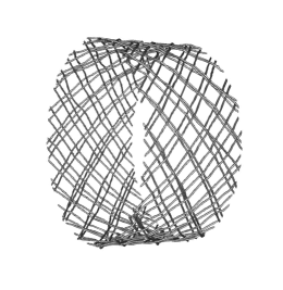
Figure 1: A sketch of stented arteries: with a collateral artery (left), an aneurysmal sac (middle) and a 3D example of a real metallic multi-wired stent (right)

From the applicative point of view these two situations are of interest since they represent a dual constraint that a stent should optimize somehow: the grid generated by the wires should be coarse enough to provide blood to the collateral arteries (for instance iliac arteries in the aorta), at the same time the wires should be close enough to have a real effect in terms of velocity reduction in the aneurysm.

Multi-layer metallic wired stents seem to satisfy both the constraints at the same time. Although experimentally exhibited [4, 26], these facts needed a better mathematical understanding. We give here results in this sense, setting a common framework for both phenomena in the case of the Stokes flow.

Inspired by homogenization techniques applied to the case of rough boundaries [1, 22, 29] we construct a first-order multi-scale approximation of the velocity and the pressure. By averaging, we get a first order accurate macroscopic description of the fluid flow. Indeed, we compute an explicit expression of the velocity through the fictitious interface supporting the stent and separating the main artery from the contiguous zone. This formula only depends on the input data of the problem and some homogenized constants obtained solving microscopic cell problems. In the case of the aneurysmal sac we show rigorously that the zero order pressure in the sac is constant and averaged with respect to the pressure in the main artery, which was not known. Then we show that formally this leads also to redefine the problem in a new and implicit way in the domain decomposition flavor. Actually we obtain a new set of interface conditions along the fictitious interface: while for the normal velocity they look similar to those presented in [10, 2, 9], the tangential conditions are new to our knowledge. They express a slip velocity in the main artery (as in [20]), but a discontinuous homotetic relationship between horizontal velocities across the interface of the stent (see system (5)). Our results concern the steady Stokes equations, as in [2], the same interface conditions are valid in the case unsteady Navier-Stokes case.

From the mathematical point of view this paper introduces several novelties. The case of a sieve has been widely studied in a different setting in [11, 12, 2, 9, 6]. In these works, the authors considered no-slip obstacles set on a surface with various dimensionalities but with a common point: the velocity was completely imposed at the inlet/outlet boundaries of the fluid domain. Although this could seem a technicality, it influences drastically the limiting regime of the flow. Indeed a complete velocity profile is imposed as a Dirichlet condition at the inlet/outlet of the domain, so that the total flow-rate through the sieve remains constant whatever $\epsilon$, the size of the obstacles: a resistive term appears as a zeroth order limit in the fluid equations. In the context of blood flow such a regime seems hard to reach: experiences show that when the wires are to dense no transverse flow crosses the stent. This suggests that through the porous interface, blood flow should be driven by a pressure drop more that a fixed flow-rate.

In this direction, Jäger and Mikelić considered a pressure driven fluid in [19]. But they studied an interface whose thickness was independent on $\epsilon$, which seemed useless for our purpose : the diameter of the wires of the stent are dependent on the radius of the artery where the stent should be implanted. It appears natural to consider roughness size that varies wrt $\epsilon$ in any direction. Moreover in this paper we introduce both a tangential and a transverse flow along and trough the stent. Indeed, in the limiting regime considered by Jäger and Mikelić [19], the velocity is zero. Here when the collateral artery or a sac are completely closed by the stent, we still expect a Poiseuille profile in the main artery.

At a more technical level, this work improves the approach developed in [5, 27] in order to correct edge oscillations introduced by periodic boundary layers. At the same time, we give an appropriate framework to deal with this problem in the case of Stokes equations. Indeed, due to the presence of the obstacles, the divergence operator is singular wrt $\epsilon$, this implies degradation of convergence results when lifting the non-free divergence terms and estimating the pressure. In this frame, we decompose the corrections of the superfluous boundary layer oscillations in two parts :

• on the microscopic side we use weighted Sobolev spaces to describe the behaviour at infinity of the vertical corner correctors, defined on a half plane. This provides accurate decay rates with respect to $\epsilon$ at the macroscopic level near the corner. Indeed, using onto mappings between weighted Sobolev spaces we improve decay estimates already derived in the scalar case in [5, 27]. Then in the spirit of [2] we construct a microscopic lifting operator that allows the vertical correctors to fullfil the Dirichlet condition on the obstacles,

• a complementary macroscopic corrector is added in a second step, that handles exponentially decreasing errors far from the corners.

An attempt to break the periodicity at the inlet/outlet of the domain was done in [20] by using a vertical corrector localized in a tiny strip near the vertical interface. But, decay estimates claimed in formula (77) p. 1123 [20] seem to work, to our knowledge, only for a priori estimates of the error and are not accurate enough to be used in the very weak estimates.

We underline as well that in the literature [20, 21, 22, 23] error estimates between the direct rough solution and the approximations constructed thanks to boundary layer arguments concerned the ${\bf L}^{2}$ norm of the velocity. In this paper we provide error estimates of the same order for the pressure as well in the negative Sobolev $H^{-1}$ norm. This is obtained using the microscopic nature of the pressure correctors and in particular thanks to the very precise control of lateral correctors. We stress that these vertical correctors play a crucial part in our error analysis at several steps of this work.

The paper is organized as follows: in the two next sections, after some basic notations and definitions, we give a detailed review of the results obtained either in the case of a collateral artery or a sacular aneurysm. We give in section 4 the abstract results that are used in section 5 in order to prove the claims. We provide numerical results showing a first order accuracy also in the discrete case in section 6. In Appendix A, we give proofs of existence, uniqueness and a priori estimates for vertical correctors in the weighted Sobolev spaces, while in Appendix B we detail the results claimed for the periodic boundary layers throughout the paper.

2 Geometry and problem settings

2.1 Geometry

In this study we consider two space dimensions. Let us define by ${\cal J}_{s}$ one or more solid obstacles included in ${\cal J}:=]0,1[^{2}$ of Lipschitz boundaries denoted $P$ in the sense of the definition p. 13-14 of Chap. 1 in [28]. We denote by ${\cal J}_{f}:=]0,1[^{2}\setminus{\cal J}_{s}$ the complementary fluid part of ${\cal J}_{s}$ in $]0,1[^{2}$. Also, we consider a smooth surface $\gamma_{M}$ strictly contained in ${\cal J}_{s}$ and enclosing $P$ and we denote ${\cal J}_{M}$ the domain contained between $\gamma_{M}$ and $P$. Then we define:

1. Macroscopic domains:

   The $\epsilon$-periodic repetition of ${\cal J}_{f}$ is denoted by ${\cal L}_{\epsilon}$ and reads:

   $${\cal L}_{\epsilon}:=\cup_{i=0}^{m}\epsilon((i,0)+{\cal J}_{f}),\text{ where }m:=\frac{1}{\epsilon},$$

   the real $\epsilon$ is always chosen such that $m$ is an integer. Then we set:

   $$\Omega_{1}:=]0,1[^{2}, {\Gamma_{\rm in}}:=\{0\}\times]0,1[,$$

   $$\Omega_{1}^{\prime}:=]0,1[\times]\epsilon,1[, \Gamma_{\rm out,1}:=\{1\}\times]0,1[,$$

   $$\Omega_{1,\epsilon}:=\Omega_{1}^{\prime}\cup(]0,1[\times\{\epsilon\})\cup{\cal L}_{\epsilon}, \Gamma_{\rm out,2}:=]0,1[\times\{-1\},$$

   $$\Omega_{2}:=]0,1[\times]-1,0[, \Gamma_{1}:=]0,1[\times\{1\},$$

   $${\Gamma_{0}}:=]0,1[\times\{0\}, \Gamma_{2}:=\{0\}\times]-1,0[\cup\{1\}\times]-1,0[,$$

   $$\Omega:=\Omega_{1}\cup{\Gamma_{0}}\cup\Omega_{2}, \Gamma_{D}:=\Gamma_{1}\cup\Gamma_{2}\cup{\Gamma_{\epsilon}},$$

   $$\Omega_{\epsilon}:=\Omega_{1,\epsilon}\cup{\Gamma_{0}}\cup\Omega_{2}, \Gamma_{N}:={\Gamma_{\rm in}}\cup\Gamma_{\rm out,1}\cup\Gamma_{\rm out,2},$$

   $$\Omega^{\prime}:=\Omega_{1}^{\prime}\cup\Omega_{2}, {\cal E}_{\epsilon}:=]0,1[\times]0,\epsilon[.$$

   The spatial variable giving the position of a point in domains above is a vector called $x$.

2. The microscopic cell domain:

   As the problem contains a solid interface surrounded by a fluid, the microscopic cell problems are set on an infinite strip $Z$ defined as follows

   $$Z^{-}:=]0,1[\times]-\infty,0[,$$

   $$\Sigma:=]0,1[\times\{0\},$$

   $$Z^{+}:=]0,1[\times\mathbb{R}_{+}\setminus{\cal J}_{s},$$

   $$Z:=Z^{+}\cup\Sigma\cup Z^{-},$$

   $$Z_{\gamma,\nu}:=Z\cap]0,1[\times]\gamma,\nu[, (\gamma,\nu)\in\mathbb{R}^{2}\text{ s.t. }\gamma<\nu.$$

   The microscopic position variable is denoted by $y:=x/\epsilon$.

3. The “corner” microscopic domain:

   In order to handle periodic perturbations on the lateral boundaries ${\Gamma_{\rm in}}\cup\Gamma_{2}\cup\Gamma_{\rm out,1}$ one needs to define a microscopic zoom near the corners $O:=(0,0)$ and $\overline{x}:=(1,0)$ of $\Omega_{\epsilon}$. This leads to set the half-plane $\Pi$ and the corresponding boundaries as

   $$\Pi:=\mathbb{R}_{+}\times\mathbb{R}$$

   $$N:=\{0\}\times]0,+\infty[,$$

   $$D:=\{0\}\times]-\infty,0[,$$

If we choose the obstacle ${\cal J}_{s}$ to be a single disk, then a graphical illustration depicts the definitions above in fig. 2 for $\epsilon=1/11$.

Figure 2: The macroscopic domains $\Omega_{\epsilon}$ (left) and $\Omega$ (middle) and the microscopic infinite strip $Z$ (right)

The exterior normal vector to any domain is denoted by ${\bf n}$, if not stated explicitly ${\bf n}$ is orientated from $\Omega_{1}$ towards $\Omega_{2}$ on the fictitious interface ${\Gamma_{0}}$. The tangent vector is defined as ${{\bf\tau}}$.

2.2 Notations and definitions

1. Any two-dimensional vector is denoted by a bold symbol: ${\mathbf{u}}:=(u_{1},u_{2})$, and single components are scalar and are not bold. The same holds for the function spaces these vectors belong to: bold letters denote vector spaces, for instance ${\bf{L}}^{2}(\Omega):=(L^{2}(\Omega))^{2}$.

2. If $\eta\in H^{1}_{{{\rm loc}}}(Z)$ then we set

   $${\overline{\eta}}(y_{2}):=\int_{0}^{1}\eta(y_{1},y_{2})dy_{1},\quad y_{2}\in\mathbb{R},$$

   to be the horizontal average of a function defined on the infinite periodic strip $Z$. Moreover by the double bar we denote a piecewise constant function defined on $Z$ as

   $$\overline{{\overline{\eta}}}(y):={\overline{\eta}}(+\infty)\mathbbm{1}_{Z^{+}}(y)+{\overline{\eta}}(-\infty)\mathbbm{1}_{Z^{-}}(y),\quad y\in Z,$$

   whenever the function ${\overline{\eta}}(\cdot)$ admits finite limits when $|y_{2}|\to\infty$. We need the values of the above function near the origin, thus we set also:

   $$\overline{{\overline{\eta}}}^{\pm}:=\overline{{\overline{\eta}}}(0^{\pm}).$$

3. For any pair $({\mathbf{u}},p)\in{\bf{L}}^{2}(\Omega)\times H^{-1}(\Omega)$ we denote by $\sigma_{{\mathbf{u}},p}$ the $2\times 2$ distributional matrix reading

   $$\sigma_{{\mathbf{u}},p}(x):=\nabla{\mathbf{u}}-p{\rm Id}_{2},\text{ a.e. }x\in\Omega,$$

   where ${\rm Id}_{2}$ is the identity matrix in $\mathbb{R}^{2}$. The tensor $\sigma_{{\mathbf{u}},p}$ looks like the stress tensor but it is not symmetric. This is due to the incompressibility constraint: the Stokes problem can still be put in the divergence form with the definition of $\sigma_{{\mathbf{u}},p}$ above.

4. The brackets $[\cdot]$ denote throughout the whole paper the jump of the quantity enclosed across fictitious interfaces: across ${\Gamma_{0}}$ on the macroscopic scale, or across $\Sigma$ on the microscopic scale, so that for instance

   $$[\sigma_{{\mathbf{u}},p}]:=\sigma_{{\mathbf{u}},p}(x_{1},0^{+})-\sigma_{{\mathbf{u}},p}(x_{1},0^{-}),\text{ while }[\overline{{\overline{\eta}}}]:=\overline{{\overline{\eta}}}^{+}-\overline{{\overline{\eta}}}^{-}.$$

5. For every microscopic function $\eta$ defined on either $Z$ or $\Pi$, we denote by

   $$\eta_{\epsilon}(x)=\eta\left(\frac{x}{\epsilon}\right),\quad\forall x\in\Omega_{\epsilon}.$$

We also need cut-off functions that we define here:

1. The cut-off $\phi$ is a scalar function $\phi:\mathbb{R}_{+}\to[0,1]$ s.t. $\phi$ is a $C^{\infty}(\mathbb{R}_{+})$ monotone decreasing function and

   $$\phi(z):=\left\{\begin{aligned} 1\text{ if }z\leq 1,\\ 0\text{ if }z\geq 2,\\ \end{aligned}\right.$$

   for any positive real $z$.

2. The “corner” cut-off functions : set $\psi_{1}:=\overline{\psi}(x)$ and $\psi_{2}:=\overline{\psi}(x-\overline{x})$ and $\overline{\psi}$ is a radial monotone decreasing cut-off function such that

   $$\overline{\psi}(x):=\left\{\begin{aligned} 1\text{ if }|x|\leq\frac{1}{3},\\ 0\text{ if }|x|\geq\frac{2}{3},\\ \end{aligned}\right.\quad\forall x\in\mathbb{R}^{2}.$$

   Finally set $\psi(x):=\psi_{1}(x)+\psi_{2}(x)$. Note that with this definition $\,\partial_{\bf n}\overline{\psi}\,=0$ on ${\Gamma_{\rm in}}\cup\Gamma_{\rm out,1}$.

3. The “far from the corner” cut-off function : $\Phi$ is defined in a complementary manner on ${\Gamma_{\rm in}}\cup\Gamma_{\rm out,1}\cup\Gamma_{2}$ such that

   $$\left\{\begin{aligned} &\psi+\Phi=1,\quad\text{ on }{\Gamma_{\rm in}}\cup\Gamma_{\rm out,1}\cup\Gamma_{2},\\ &\,\partial_{\bf n}\Phi\,=0\quad\text{ on }{\Gamma_{\rm in}}\cup\Gamma_{\rm out,1},\end{aligned}\right.$$

   and one shall take for instance $\Phi(x):=1-\psi(0,x_{2})$ for all $x$ in $\Omega$.

4. For regularity purposes we set $\lambda_{\epsilon}$ to be a cut-off function in the $\epsilon$-neighborhood of the corners $O$ and $\overline{x}$ (p. 1122 [20]). First we set at the microscopic level:

   $$\lambda(y):=|y_{2}|\mathbbm{1}_{B(O,1)}(y)+\frac{y_{2}}{|y|}\mathbbm{1}_{\{\Pi\setminus B(O,1)\}}(y),\quad\forall y\in\Pi,$$

   then we define

   $$\lambda_{\epsilon}(x):=\lambda\left(\frac{x}{\epsilon}\right)\psi_{1}(x)+\lambda\left(\frac{1-x_{1}}{\epsilon},\frac{x_{2}}{\epsilon}\right)\psi_{2}(x)+\Phi(x),\quad\forall x\in\Omega.$$

   and an easy computation shows that

   $${\left\|{\lambda_{\epsilon}}\right\|}_{H^{1}(\Omega)}\leq k\{|\log(\epsilon)|^{\frac{1}{2}}+1\},$$ (1)

   where the constant $k$ does not depend on $\epsilon$.

3 Main results

3.1 The case of a collateral artery

We study the problem : find $({\bf u}_{\epsilon},p_{\epsilon})$ solving the stationary Stokes equations

$$\left\{\begin{aligned} &-\Delta{\bf u}_{\epsilon}+\nabla p_{\epsilon}=0&\text{ in }\Omega_{\epsilon},\\ &{\rm div\,}{\bf u}_{\epsilon}=0&\text{ in }\Omega_{\epsilon},\\ &p_{\epsilon}=p_{\rm in}\text{ on }{\Gamma_{\rm in}},\quad p_{\epsilon}={p_{{\rm out},1}}\text{ on }\Gamma_{\rm out,1},&p_{\epsilon}={p_{{\rm out},2}}\text{ on }\Gamma_{\rm out,2},\\ &{\bf u}_{\epsilon}\cdot{\bf\tau}=0&\text{ on }{\Gamma_{\rm in}}\cup\Gamma_{\rm out,1}\cup\Gamma_{\rm out,2},\\ &{\bf u}_{\epsilon}=0&\text{ on }\Gamma_{1}\cup\Gamma_{2}\cup{\Gamma_{\epsilon}},\\ \end{aligned}\right.$$ (2)

Because of the microscopic structure of ${\Gamma_{\epsilon}}$, the solution of such a system is complex and expensive from the numerical point of view. For this reason throughout this article we use homogenization in order to construct approximations of $({\bf u}_{\epsilon},p_{\epsilon})$. This technique decomposes in two steps :

1. the derivation of a multi-scale asymptotic expansion and the construction of an averaged macroscopic approximation. The first part can be seen as an iterative algorithm with respect to powers of $\epsilon$ :

   1. pass to the limit with respect to $\epsilon$ and obtain a macroscopic zero order approximation. In our case, because of the straight geometry of the main artery and of the boundary conditions, the Poiseuille profile is obtained in $\Omega_{1}$ and a trivial solution in $\Omega_{2}$ :

      $$\left\{\begin{aligned} &{\bf u}_{0}(x)=\frac{p_{\rm in}-{p_{{\rm out},1}}}{2}(1-x_{2})x_{2}{\mathbf{e}}_{1}\mathbbm{1}_{\Omega_{1}},\\ &p_{0}(x)=(p_{\rm in}(1-x_{1})+{p_{{\rm out},1}}x_{1})\mathbbm{1}_{\Omega_{1}}+{p_{{\rm out},2}}\mathbbm{1}_{\Omega_{2}},\end{aligned}\right.\quad\forall x\in\Omega,$$ (3)

   2. construct microscopic boundary layers correcting errors made by the zeroth order approximation on ${\Gamma_{\epsilon}}$ and ${\Gamma_{0}}$: we set up in the next section three boundary layers $({\boldsymbol{\beta}},\pi),({\boldsymbol{\Upsilon}},\varpi)$ and $({\boldsymbol{\chi}},\eta)$ to this purpose. These functions solve periodic microscopic problems (14), (15) and (16) on the strip $Z$.

   3. compute the constants that these correctors reach at $y_{2}=\pm\infty$: $(\overline{\overline{{\boldsymbol{\beta}}}}^{\pm},0)$, $(\overline{\overline{\boldsymbol{\Upsilon}}}^{\pm},0)$ and $(\overline{\overline{{\boldsymbol{\chi}}}},\overline{{\overline{\eta}}}^{\pm})$. Then subtract them to the correctors. Physically, $\overline{\overline{{\boldsymbol{\beta}}}}^{\pm},\overline{\overline{\boldsymbol{\Upsilon}}}^{\pm}$ provide a microscopic feed-back relative to the horizontal velocity (see the wall-law framework in [29, 20] and references therein) whereas the pressure difference $[\overline{{\overline{\eta}}}]$ represents a microscopic resistivity in the flavor of [2, 9, 6].

   4. take into account the homogenized constants on the limit interface ${\Gamma_{0}}$ by solving a macroscopic problem: find $({\bf u}_{1},p_{1})$ s.t.

      $$\left\{\begin{aligned} -&\Delta{\bf u}_{1}+\nabla p_{1}=0&\text{ in }\Omega_{1}\cup\Omega_{2},\\ &{\rm div\,}{\bf u}_{1}=0&\text{ in }\Omega_{1}\cup\Omega_{2},\\ &{\bf u}_{1}=0&\text{ on }\Gamma_{1}\cup\Gamma_{2},\\ &\left.\begin{aligned} &{\bf u}_{1}\cdot{\bf\tau}=0\\ &p_{1}=0\end{aligned}\right\}&\text{ on }\Gamma_{N},\\ &{\bf u}_{1}(x_{1},0^{\pm})=\left(\frac{\partial u_{0,1}}{\partial x_{2}}(x_{1},0^{+})\overline{\overline{\beta}}^{\pm}_{1}+\left[\frac{\partial u_{0,1}}{\partial x_{2}}\right]\overline{\overline{\Upsilon}}^{\pm}_{1}\right){\mathbf{e}}_{1}+\frac{[p_{0}]}{[\overline{{\overline{\eta}}}]}\overline{\overline{\chi}}_{2}{\mathbf{e}}_{2}&\text{ on }{\Gamma_{0}}^{\pm}\end{aligned}\right.$$ (4)

      This macroscopic corrector depends on the zeroth order approximation and the homogenized constants. Due to the explicit form of the Poiseuille profile, the Dirichlet data is explicit on both sides of ${\Gamma_{0}}$, (nevertheless the solution $({\bf u}_{1},p_{1})$ is not explicit inside $\Omega_{1}\cup\Omega_{2}$).

   5. go to (1b) and correct, on a micrscopic scale, errors made by $({\bf u}_{1},p_{1})$ on ${\Gamma_{\epsilon}}\cup{\Gamma_{0}}$ in order to get higher order terms in the asymptotic ansatz.

2. The second step consists then in averaging this ansatz and obtaining an expansion of the macroscopic solutions only. This gives, for instance, at first order :

   $${\bf\overline{u}}_{\epsilon}(x):={\bf u}_{0}(x)+\epsilon{\bf u}_{1}(x),\quad\overline{p}_{\epsilon}(x):=p_{0}(x)+\epsilon p_{1}(x),\quad\forall x\in\Omega_{1}\cup\Omega_{2}.$$

   In particular as ${\bf\overline{u}}_{\epsilon}\cdot{\bf n}=\epsilon[p_{0}]/[\overline{{\overline{\eta}}}]$ on ${\Gamma_{0}}$, one gets an explicit first order velocity profile across ${\Gamma_{0}}$. As a consequence, we obtain a new result :

   Proposition 1.

   The flow-rate in the collateral artery $\Omega_{2}$ can be computed explicitly and reads

   $$Q_{{\Gamma_{0}}}:=\int_{\Gamma_{0}}{\bf\overline{u}}_{\epsilon}\cdot{\bf n}dx_{1}=\frac{\epsilon}{\left[\overline{{\overline{\eta}}}\right]}\int_{\Gamma_{0}}[p_{0}]dx_{1}=\frac{\epsilon}{\left[\overline{{\overline{\eta}}}\right]}\int_{\Gamma_{0}}({p_{{\rm out},1}}+(p_{\rm in}-{p_{{\rm out},1}})(1-x_{1})-{p_{{\rm out},2}})\,dx_{1}$$

   As stated above $[\overline{{\overline{\eta}}}]$ depends only on the geometry of the microscopic obstacle ${\cal J}_{s}$ and is independent of any other parameter. In the last section of this paper we give some numerical examples that illustrate the accuracy of this result (see fig. 9 and 10). Note that the zeroth order approximation does not provide any transverse flow through ${\Gamma_{0}}$. Although our results provide a first order correction, we underline that in the physiological context the pressures $(p_{\rm in},{p_{{\rm out},1}})$ present in the main artery can be very important compared to ${p_{{\rm out},2}}$ : the first order flow rate $Q_{{\Gamma_{0}}}$ can thus be quantitatively significant as well.

In this work we constructed an suitable mathematical framework in order to analyse the error made in the two main steps of the construction above. This allows to state the main result of this paper:

Theorem 3.1.

There exists a unique pair $({\bf u}_{\epsilon},p_{\epsilon})\in{\bf H}^{1}(\Omega_{\epsilon})\times L^{2}(\Omega_{\epsilon})$ solving problem (2). The averaged asymptotic ansatz $({\bf\overline{u}}_{\epsilon},\overline{p}_{\epsilon})$ belongs to ${\bf L}^{2}(\Omega_{j})\times H^{-1}(\Omega_{j})$ for $j\in\{1,2\}$ and satisfies the convergence result

$${\left\|{{\bf u}_{\epsilon}-{\bf\overline{u}}_{\epsilon}}\right\|}_{L^{2}(\Omega_{1}\cup\Omega_{2})}+{\left\|{p_{\epsilon}-\overline{p}_{\epsilon}}\right\|}_{H^{-1}(\Omega_{1}^{\prime}\cup{\cal L}_{\epsilon}\cup\Omega_{2})}\leq k\epsilon^{\frac{3}{2}^{-}},$$

where $\frac{3}{2}^{-}$ represent any real number strictly less then $\frac{3}{2}$ and the constant $k$ is independent on $\epsilon$.

Expressing interface conditions satisfied by $({\bf\overline{u}}_{\epsilon},\overline{p}_{\epsilon})$ on ${\Gamma_{0}}$ in an implicit way and neglecting higher order rests, we show formally that in fact $({\bf\overline{u}}_{\epsilon},\overline{p}_{\epsilon})$ solve at first order a new interface problem :

$$\left\{\begin{aligned} &-\Delta{\bf\overline{u}}_{\epsilon}+\nabla\overline{p}_{\epsilon}=0&\text{ in }\Omega_{1}\cup\Omega_{2},\\ &{\rm div\,}{\bf\overline{u}}_{\epsilon}=0&\text{ in }\Omega_{1}\cup\Omega_{2},\\ &{\bf\overline{u}}_{\epsilon}=0&\text{ on }\Gamma_{1}\cup\Gamma_{2},\\ &{\bf\overline{u}}_{\epsilon}\cdot{\bf\tau}=0&\text{ on }\Gamma_{N},\\ &\overline{p}_{\epsilon}=p_{\rm in},\text{ on }{\Gamma_{\rm in}},\quad\overline{p}_{\epsilon}={p_{{\rm out},1}}\text{ on }\Gamma_{\rm out,1},\quad\overline{p}_{\epsilon}={p_{{\rm out},2}}&\text{ on }\Gamma_{\rm out,2},\\ &\left.\begin{aligned} &{\bf\overline{u}}_{\epsilon}^{+}\cdot{\bf\tau}=\epsilon(\overline{\overline{\beta}}^{+}_{1}+\overline{\overline{\Upsilon}}^{+}_{1})\frac{\partial\overline{u}_{\epsilon,1}}{\partial x_{2}}^{+},\quad\frac{{\bf\overline{u}}_{\epsilon}^{+}\cdot{\bf\tau}}{\overline{\overline{\beta}}^{+}_{1}+\overline{\overline{\Upsilon}}^{+}_{1}}=\frac{{\bf\overline{u}}_{\epsilon}^{-}\cdot{\bf\tau}}{\overline{\overline{\beta}}^{-}_{1}+\overline{\overline{\Upsilon}}^{-}_{1}}\\ &{\bf\overline{u}}_{\epsilon}^{+}\cdot{\bf n}={\bf\overline{u}}_{\epsilon}^{-}\cdot{\bf n}=-\frac{\epsilon}{[\overline{{\overline{\eta}}}]}([\sigma_{{\bf\overline{u}}_{\epsilon},\overline{p}_{\epsilon}}]\cdot{\bf n},{\bf n})\end{aligned}\right\}&\text{ on }{\Gamma_{0}}.\end{aligned}\right.$$ (5)

The horizontal velocity on ${\Gamma_{0}}^{+}$ is related to the shear rate trough a kind of mixed boundary condition alike to the Beaver, Joseph and Saffeman condition [20]. This implicit relationship accounts for the friction effect due to the obstacles that “resist” to the flow in the main artery. Nevertheless because the interface separates two domains $\Omega_{1}$ and $\Omega_{2}$, we obtain a second expression between the upper and the lower horizontal velocities $\overline{u}_{\epsilon,1}^{+}$ and $\overline{u}_{\epsilon,1}^{-}$: they are proportional and thus discontinuous. To our knowledge this is new.

On the other hand, the interface condition on the normal velocity could be integrated in the Stokes equations as a kind of “strange term” in the spirit of [10, 2], but as we are at first order with respect to $\epsilon$: (i) the strange term is divided by $\epsilon$ (in [10, 2] this is a zero order term independent on $\epsilon$ ) (ii) the derivation does not follow at all the same argumentation. In a forthcoming work we study the well-posedness of such a system as well as its consistency with respect to $({\bf\overline{u}}_{\epsilon},\overline{p}_{\epsilon})$ and $({\bf u}_{\epsilon},p_{\epsilon})$. Because of the particular signs of the homogenized constants but also the discontinuous nature of the interface conditions in the tangential direction to ${\Gamma_{0}}$, this seems a challenging task.

3.2 The case of an aneurysm

The framework introduced above can be extended to the case of an aneurysm; considering the same domain $\Omega_{\epsilon}$ as above we define a new problem : find $({\bf u}_{\epsilon},p_{\epsilon})$ solving

$$\left\{\begin{aligned} &-\Delta{\bf u}_{\epsilon}+\nabla p_{\epsilon}=0&\text{ in }\Omega_{\epsilon},\\ &{\rm div\,}{\bf u}_{\epsilon}=0&\text{ in }\Omega_{\epsilon},\\ &p_{\epsilon}=p_{\rm in}\text{ on }{\Gamma_{\rm in}},&p_{\epsilon}={p_{{\rm out},1}}\text{ on }\Gamma_{\rm out,1},\\ &{\bf u}_{\epsilon}\cdot{\bf\tau}=0&\text{ on }{\Gamma_{\rm in}}\cup\Gamma_{\rm out,1},\\ &{\bf u}_{\epsilon}=0&\text{ on }\Gamma_{1}\cup\Gamma_{2}\cup\Gamma_{\rm out,2}.\\ \end{aligned}\right.$$ (6)

The main difference resides in the boundary condition imposed on $\Gamma_{\rm out,2}$ : here we impose a complete adherence condition on the velocity ; this closes the output $\Gamma_{\rm out,2}$ and transforms the collateral artery into an idealized square aneurysm.

Again, we construct a similar multi-scale asymptotic ansatz. We extract the macroscopic part to get a homogenized expansion $({\bf\overline{u}}_{\epsilon},\overline{p}_{\epsilon})$ reading

$${\bf\overline{u}}_{\epsilon}(x):={\bf u}_{0}(x)+\epsilon{\bf u}_{1}(x),\quad\overline{p}_{\epsilon}(x):=p_{0}(x)+\epsilon p_{1}(x),\quad\forall x\in\Omega_{1}\cup\Omega_{2},$$

where $({\bf u}_{0},p_{0})$ is again a Poiseuille profile but complemented by an unknown constant pressure $p_{0}^{-}$ inside the sac:

$$\left\{\begin{aligned} &{\bf u}_{0}(x)=\frac{p_{\rm in}-{p_{{\rm out},1}}}{2}(1-x_{2})x_{2}{\mathbf{e}}_{1}\mathbbm{1}_{\Omega_{1}}\\ &p_{0}(x)=p_{0}^{+}(x)\mathbbm{1}_{\Omega_{1}}+p_{0}^{-}\mathbbm{1}_{\Omega_{2}},\\ &p_{0}^{+}(x):={p_{{\rm out},1}}+(p_{\rm in}-{p_{{\rm out},1}})(1-x_{1}),\quad p_{0}^{-}\in\mathbb{R}\end{aligned}\right.,\quad\forall x\in\Omega$$ (7)

Then again $({\bf u}_{1},p_{1})$ solves a mixed Stokes problem (4), the only difference being that ${\bf u}_{1}=0$ on $\Gamma_{\rm out,2}$. This gives again a new result:

Corollary 3.1.

The zeroth order pressure is constant in $\Omega_{2}$, moreover it satisfies the following compatibility condition with respect to the pressure in the main artery:

$$p_{0}^{-}=\frac{1}{|{\Gamma_{0}}|}\int_{\Gamma_{0}}p_{0}^{+}(x_{1},0)\,dx_{1}.$$

This gives an explicit velocity profile on ${\Gamma_{0}}$ which reads:

$${\bf\overline{u}}_{\epsilon}\cdot{\bf n}=\frac{\epsilon}{[\overline{{\overline{\eta}}}]}(p_{0}^{+}(x_{1},0)-p_{0}^{-})+O(\epsilon^{2}).$$

The interface condition exhibited on the normal velocity shows rigorously a phenomenon already observed experimentally [4, 26]. Set $x_{1,\max}:=\max_{x\in{\Gamma_{0}}}x_{1}$ (resp. $x_{1,\min}:=\min_{x\in{\Gamma_{0}}}x_{1}$) and $\overline{x}_{1}:=(x_{1,\max}+x_{1,\min})/2$, when $x_{1}<\overline{x}_{1}$ the pressure jump $[p_{0}]:=p_{0}^{+}(x)-p_{0}^{-}$ is positive, otherwise it is negative. This implies that the first order flow trough the stent is entering $\Omega_{2}$ when $x_{1}<\overline{x}_{1}$ and leaving it otherwise. Thus the prosthesis inverses the orientation of the cavitation in $\Omega_{2}$ with respect to the non-stented artery (see fig. 3).

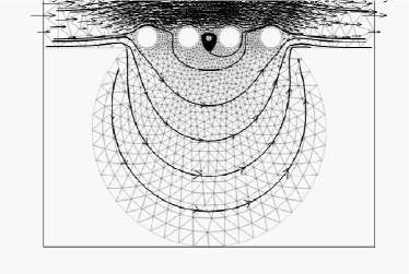
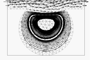
Figure 3: Streamlines and velocity vectors in an aneurysmal sac, with (left) and without a stent (right)

As stated in the corollary, we show in the next section that in fact the zero order pressure is the only constant that insures conservation of mass in $\Omega_{2}$. From the medical point of view the two claims on pressure and flow are of interest. They quantify and confirm the stabilizing effect of a porous stent: besides reducing the stress on the wall of the aneurysm,the stent averages also the pressure inside the sac avoiding for instance corner singularities (see fig. 4).

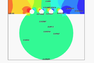
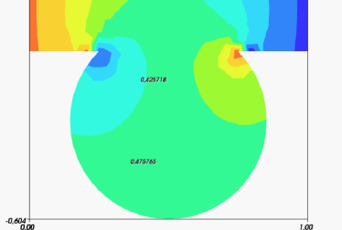
Figure 4: Pressure in an aneurysmal sac, with (left) and without a stent (right)

The geometry presented as an illustration in figures 3 and 4 does not fit exactly in the hypotheses of section 2.1: the main difference is the curved circular form of the boundaries of $\Omega_{2}$. Nevertheless the phenomenon observed when $\Omega_{2}$ is the square $]0,1[\times]-1,0[$ still happens when $\Omega_{2}$ has this more physiological shape.

Again one has a mathematical validation of the formal multi-scale construction

Theorem 3.2.

There exists a unique pair $({\bf u}_{\epsilon},p_{\epsilon})\in{\bf H}^{1}(\Omega_{\epsilon})\times L^{2}(\Omega_{\epsilon})$ solving (6). The first order approximation $({\bf\overline{u}}_{\epsilon},\overline{p}_{\epsilon})$ belongs to ${\bf L}^{2}(\Omega_{1}\cup\Omega_{2})\times H^{-1}(\Omega_{1}\cup\Omega_{2})$, moreover we have a convergence result that reads

$${\left\|{{\bf u}_{\epsilon}-{\bf\overline{u}}_{\epsilon}}\right\|}_{L^{2}(\Omega)}+{\left\|{p_{\epsilon}-\overline{p}_{\epsilon}}\right\|}_{H^{-1}(\Omega^{\prime}\cup{\cal L}_{\epsilon})}\leq k\epsilon^{\frac{3}{2}^{-}},$$

where $\frac{3}{2}^{-}$ represent any real number strictly less then $\frac{3}{2}$, the constant $k$ depends on the data of the problem and the domain but not on $\epsilon$.

We show the same type of result as above : $({\bf\overline{u}}_{\epsilon},\overline{p}_{\epsilon})$ solve formally the same implicit problem (5) up to the second order error, but with a homogeneous Dirichlet condition on $\Gamma_{\rm out,2}$.

4 Technical preliminaries

In this section we introduce the basic results that allow to deal with the Stokes problem on a perforated domain $\Omega_{\epsilon}$ together with the specific boundary conditions as in (2).

4.1 Weak solutions for sieve problems

In the spirit of Appendix in [30] we start by the definition a restriction operator $R_{\epsilon}$ acting on functions defined in $\Omega$ and providing resulting functions defined on $\Omega_{\epsilon}$ and vanishing on ${\Gamma_{\epsilon}}$.

Definition 1.

Let $\boldsymbol{V}:=\{{\bf v}\in{\bf H}^{1}(\Omega_{\epsilon})\text{ s.t. }{\bf v}=0\text{ on }\Gamma_{D}\text{ and }{\bf v}\cdot{\bf\tau}=0\text{ on }\Gamma_{N}\}$, and we endow it with the usual ${\bf H}^{1}$ norm. The tilde operator refers always to an extension by zero outside $\Omega_{\epsilon}$ i.e.

$$\forall{\mathbf{u}}\in\boldsymbol{V},\tilde{{\mathbf{u}}}\in{\bf H}^{1}(\Omega)\text{ s.t. }\tilde{{\mathbf{u}}}:=\left\{\begin{aligned} {\mathbf{u}}&\text{ if }x\in\Omega_{\epsilon}\\ 0&\text{ otherwise }\end{aligned}\right.$$

We define the restriction operator $R_{\epsilon}\in{\cal L}({\bf H}^{1}(\Omega);{\bf H}^{1}(\Omega_{\epsilon}))$ s.t.

1. ${\mathbf{u}}\in\boldsymbol{V}$ implies $R_{\epsilon}\tilde{{\mathbf{u}}}\equiv{\mathbf{u}}$,

2. ${\rm div\,}{\mathbf{u}}=0$ in $\Omega$ implies that ${\rm div\,}(R_{\epsilon}{\mathbf{u}})=0$ in $\Omega_{\epsilon}$,

3. There exist three real constants $k_{1},k_{2}$ and $k_{3}$ independent on $\epsilon$ s.t.

   $$\left\{\begin{aligned} {\left\|{R_{\epsilon}{\mathbf{u}}}\right\|}_{{\bf L}^{2}(\Omega_{\epsilon})}&\leq k_{1}\{{\left\|{{\mathbf{u}}}\right\|}_{{\bf L}^{2}(\Omega)}+\epsilon{\left\|{\nabla{\mathbf{u}}}\right\|}_{L^{2}(\Omega)^{4}}\},\\ {\left\|{\nabla R_{\epsilon}{\mathbf{u}}}\right\|}_{{\bf L}^{2}(\Omega_{\epsilon})}&\leq k_{2}\left\{\frac{1}{\epsilon}{\left\|{{\mathbf{u}}}\right\|}_{{\bf L}^{2}(\Omega)}+{\left\|{\nabla{\mathbf{u}}}\right\|}_{L^{2}(\Omega)^{4}}\right\},\\ {\left\|{\nabla R_{\epsilon}{\mathbf{u}}}\right\|}_{{\bf L}^{2}(\Omega_{\epsilon})}&\leq k_{3}\frac{1}{\sqrt{\epsilon}}{\left\|{{\mathbf{u}}}\right\|}_{{\bf H}^{1}(\Omega)}.\end{aligned}\right.$$

Lemma 2.

There exists an opertor $R_{\epsilon}$ in the sense of Definition 1

Proof.

The restriction operator $R_{\epsilon}$ is constructed exactly as in Lemma 3 and 4 in the Appendix by L. Tartar in [30], namely for a given ${\mathbf{u}}\in{\bf H}^{1}({\cal J})$ there exists a unique pair $({\bf v},q)\in{\bf H}^{1}({\cal J}_{M})\times(L^{2}({\cal J}_{M})/\mathbb{R})$ satisfying:

$$\left\{\begin{aligned} &-\Delta{\bf v}+\nabla q=-\Delta{\mathbf{u}}&\text{ in }{\cal J}_{M},\\ &{\rm div\,}{\bf v}={\rm div\,}{\mathbf{u}}+\frac{1}{|{\cal J}_{M}|}\int_{{\cal J}_{s}}{\rm div\,}{\mathbf{u}}\;dy,&\text{ in }{\cal J}_{M}\\ &{\bf v}=0&\text{ on }P,\\ &{\bf v}={\mathbf{u}}&\text{ on }\gamma_{M},\\ \end{aligned}\right.$$

There exists a constant $k$ independent on ${\mathbf{u}}$ s.t. ${\left\|{{\bf v}}\right\|}_{{\bf H}^{1}({\cal J}_{M})}\leq k{\left\|{{\mathbf{u}}}\right\|}_{{\bf H}^{1}({\cal J})}$. By setting

$$R{\mathbf{u}}(y):=\left\{\begin{aligned} {\mathbf{u}}(y)&\text{ if }y\in{\cal J}\setminus({\cal J}_{M}\cup{\cal J}_{s})\\ {\bf v}(y)&\text{ if }y\in{\cal J}_{M}\\ 0&\text{ if }y\in{\cal J}_{s}\\ \end{aligned}\right.$$

we evidently have ${\left\|{R{\mathbf{u}}}\right\|}_{{\bf H}^{1}({\cal J})}\leq k{\left\|{{\mathbf{u}}}\right\|}_{{\bf H}^{1}({\cal J})}$. and $R{\mathbf{u}}$ coincides with ${\mathbf{u}}$ if ${\mathbf{u}}\equiv 0$ on ${\cal J}_{s}$ and ${\rm div\,}{\mathbf{u}}=0$ implies ${\rm div\,}(R{\mathbf{u}})=0$.

Now let ${\mathbf{u}}\in{\bf H}^{1}(\Omega)$. For any given $x\in{\cal E}_{\epsilon}$, we set $y_{1}:=x_{1}/\epsilon-E(x_{1}/\epsilon)$, $y_{2}:=x_{2}/\epsilon$ and $i:=E(x_{1}/\epsilon)$ where $E(\cdot)$ is the lower integer part of its real argument. For each $i$ we define a function $\underline{{\mathbf{u}}}_{i}:{\cal J}\to\mathbb{R}$ s.t. $\underline{{\mathbf{u}}}_{i}(y):={\mathbf{u}}(x)$. This allows us to set $R_{\epsilon}{\mathbf{u}}$ as

$$R_{\epsilon}{\mathbf{u}}(x):=\left\{\begin{aligned} &{\mathbf{u}}(x)&\text{ if }x\in\Omega^{\prime},\\ &\sum_{i=0}^{1/\epsilon}R\underline{{\mathbf{u}}}_{i}(x_{1}/\epsilon-i,x_{2}/\epsilon)\mathbbm{1}_{\epsilon({\cal J}+i{\mathbf{e}}_{1})}(x)&\text{ if }x\in{\cal E}_{\epsilon}.\\ \end{aligned}\right.$$

This definition implies obviously that ${\left\|{R_{\epsilon}{\mathbf{u}}}\right\|}_{{\bf H}^{1}(\Omega^{\prime})}\equiv{\left\|{{\mathbf{u}}}\right\|}_{{\bf H}^{1}(\Omega^{\prime})}$ and we focus on ${\cal E}_{\epsilon}$.

$${\left\|{R_{\epsilon}{\mathbf{u}}}\right\|}_{{\bf L}^{2}({\cal L}_{\epsilon})}^{2}=\sum_{i=0}^{\frac{1}{\epsilon}}\epsilon^{2}\int_{{\cal J}_{f}+i{\mathbf{e}}_{1}}|R\underline{{\mathbf{u}}}_{i}|dy\leq k\sum_{i=0}^{\frac{1}{\epsilon}}\epsilon^{2}{\left\|{\underline{{\mathbf{u}}}_{i}}\right\|}_{{\bf H}^{1}({\cal J})}^{2}\leq k\{{\left\|{{\mathbf{u}}}\right\|}_{{\bf L}^{2}({\cal E}_{\epsilon})}^{2}+\epsilon^{2}{\left\|{\nabla_{x}{\mathbf{u}}}\right\|}_{L^{2}({\cal E}_{\epsilon})^{4}}\}.$$

The key point of the proof are now estimates on the gradient. Taking a regular function ${\mathbf{u}}\in\boldsymbol{{\cal D}}(\Omega)$, one obtains in a similar way as above:

$${\left\|{\nabla R_{\epsilon}{\mathbf{u}}}\right\|}_{L^{2}({\cal L}_{\epsilon})^{4}}\leq k\left\{\frac{1}{\epsilon}{\left\|{{\mathbf{u}}}\right\|}_{{\bf L}^{2}({\cal E}_{\epsilon})}+{\left\|{\nabla{\mathbf{u}}}\right\|}_{L^{2}({\cal E}_{\epsilon})^{4}}\right\}$$ (8)

Now one writes

$${\mathbf{u}}(x)={\mathbf{u}}(x_{1},0)+\int_{0}^{x_{2}}\partial_{x_{2}}{\mathbf{u}}(x_{1},s)ds$$

which, after taking the square, integrating on ${\cal E}_{\epsilon}$ and using Cauchy-Schwartz gives

$${\left\|{{\mathbf{u}}}\right\|}_{{\bf L}^{2}({\cal E}_{\epsilon})}^{2}\leq k\left\{\epsilon{\left\|{{\mathbf{u}}}\right\|}_{{\bf L}^{2}({\Gamma_{0}})}^{2}+\epsilon^{2}{\left\|{\nabla{\mathbf{u}}}\right\|}_{L^{2}({\cal E}_{\epsilon})^{4}}^{2}\right\},$$

thanks to the continuity of the trace operator ${\left\|{\gamma({\mathbf{u}})}\right\|}_{H^{\frac{1}{2}}(\Gamma)}\leq k{\left\|{{\mathbf{u}}}\right\|}_{{\bf H}^{1}(\Omega)}$, one has:

$${\left\|{{\mathbf{u}}}\right\|}_{{\bf L}^{2}({\cal E}_{\epsilon})}^{2}\leq k^{\prime}\left\{\epsilon{\left\|{{\mathbf{u}}}\right\|}_{{\bf H}^{1}(\Omega)}^{2}+\epsilon^{2}{\left\|{\nabla{\mathbf{u}}}\right\|}_{L^{2}({\cal E}_{\epsilon})^{4}}^{2}\right\},$$

where the constant $k^{\prime}$ does not depend on $\epsilon$. Using this last inequality in (8) ends the proof. ∎

Definition 4.1.

We define the corresponding lifting operator $S_{\epsilon}{\mathbf{u}}:=(R_{\epsilon}-{\rm Id}_{2}){\mathbf{u}}$. For every $x$ in ${\cal L}_{\epsilon}$ there exist a unique $i:=E(x/\epsilon)\in\{0,\dots,\frac{1}{\epsilon}\}$, $y_{1}=x_{1}/\epsilon-i$ and $y_{2}=x_{2}/\epsilon$ s.t. if ${\bf v}_{i}$ solves

$$\left\{\begin{aligned} &-\Delta{\bf v}_{i}+\nabla q=0&\text{ in }{\cal J}_{M}+i{\mathbf{e}}_{1},\\ &{\rm div\,}{\bf v}_{i}=\frac{1}{|{\cal J}_{M}+i{\mathbf{e}}_{1}|}\int_{{\cal J}_{s}+i{\mathbf{e}}_{1}}{\rm div\,}\underline{{\mathbf{u}}}_{i}\;dy,&\text{ in }{\cal J}_{M}+i{\mathbf{e}}_{1}\\ &{\bf v}_{i}=\underline{{\mathbf{u}}}_{i}&\text{ on }P+i{\mathbf{e}}_{1},\\ &{\bf v}_{i}=0&\text{ on }\gamma_{M}+i{\mathbf{e}}_{1},\\ \end{aligned}\right.$$

then one sets $S_{\epsilon}{\mathbf{u}}(x):=\sum_{i=0}^{\frac{1}{\epsilon}}{\bf v}_{i}(y)\mathbbm{1}_{{\cal J}_{M}+i{\mathbf{e}}_{1}}$ for every $x\in\Omega_{\epsilon}$. One has estimates similar to those of the restriction operator

$${\left\|{S_{\epsilon}{\mathbf{u}}}\right\|}_{{\bf L}^{2}(\Omega_{\epsilon})} \equiv{\left\|{S_{\epsilon}{\mathbf{u}}}\right\|}_{{\bf L}^{2}({\cal L}_{\epsilon})}\leq k\left\{{\left\|{{\mathbf{u}}}\right\|}_{L^{2}({\cal E}_{\epsilon})}+\epsilon{\left\|{\nabla{\mathbf{u}}}\right\|}_{L^{2}({\cal E}_{\epsilon})}\right\},$$

$${\left\|{\nabla S_{\epsilon}{\mathbf{u}}}\right\|}_{{\bf L}^{2}(\Omega_{\epsilon})} \equiv{\left\|{\nabla S_{\epsilon}{\mathbf{u}}}\right\|}_{{\bf L}^{2}({\cal L}_{\epsilon})}\leq\left\{\frac{1}{\epsilon}{\left\|{{\mathbf{u}}}\right\|}_{L^{2}({\cal E}_{\epsilon})}+{\left\|{\nabla{\mathbf{u}}}\right\|}_{L^{2}({\cal E}_{\epsilon})}\right\}\leq\frac{1}{\sqrt{\epsilon}}{\left\|{{\mathbf{u}}}\right\|}_{\boldsymbol{V}}\quad.$$

Proposition 3.

Let $g\in{{\rm L}}^{2}(\Omega_{\epsilon})$ there exists at least one vector ${\bf v}\in\boldsymbol{V}$ s.t.

$${\rm div\,}{\bf v}=g\text{ in }\Omega_{\epsilon},\quad{\left|{{\bf v}}\right|}_{{\bf H}^{1}(\Omega_{\epsilon})}\leq\frac{k}{\sqrt{\epsilon}}{\left\|{g}\right\|}_{L^{2}(\Omega_{\epsilon})}.$$

Proof.

We extend $g$ by zero in $\Omega\setminus\Omega_{\epsilon}$ which we denote $\tilde{g}$, we use Lemma III.3.1 and Theorem III.3.1 in [15] stating that there exists ${\bf w}\in H^{1}(\Omega)$ s.t.

$${\rm div\,}{\bf w}=\tilde{g}\text{ in }\Omega,\quad{\left|{{\bf v}}\right|}_{{\bf H}^{1}(\Omega)}\leq k{\left\|{\tilde{g}}\right\|}_{L^{2}(\Omega)},$$

where the constant $k$ does not depend on $\epsilon$. Using the restriction operator $R_{\epsilon}$ defined in the proof of Lemma 2 one sets then

$${\bf v}:=R_{\epsilon}{\bf w},$$

thanks to the estimates that the restriction operator satisfies, one gets the desired result:

$${\left|{{\bf v}}\right|}_{{\bf H}^{1}(\Omega_{\epsilon})}\leq\frac{k}{\sqrt{\epsilon}}{\left|{{\bf w}}\right|}_{{\bf H}^{1}(\Omega)}\leq\frac{k^{\prime}}{\sqrt{\epsilon}}{\left\|{\tilde{g}}\right\|}_{L^{2}(\Omega)}=\frac{k^{\prime}}{\sqrt{\epsilon}}{\left\|{g}\right\|}_{L^{2}(\Omega_{\epsilon})}.$$

∎

Thanks to the latter proposition one easily gets by duality arguments as in p. 374 in the Appendix in [30]

Proposition 4.

There exists a constant $k$ independent on $\epsilon$ s.t. for every distribution $p\in{\cal D}^{\prime}(\Omega_{\epsilon})$ s.t. $\nabla p\in\boldsymbol{V}^{\prime}$, one has

$${\left\|{p}\right\|}_{L^{2}(\Omega_{\epsilon})}\leq\frac{k}{\sqrt{\epsilon}}{\left\|{\nabla p}\right\|}_{\boldsymbol{V}^{\prime}}\;.$$

At this stage we can derive existence and uniqueness as well as a priori estimates for the solutions of the problem: given $({\bf f},g,h)\in\boldsymbol{V}^{\prime}\times L^{2}(\Omega_{\epsilon})\times H^{-{\frac{1}{2}}}(\Gamma_{N})$ find $({\mathbf{u}},p)$ s.t.

$$\left\{\begin{aligned} &-\Delta{\mathbf{u}}+\nabla p={\bf f}&\text{ in }\Omega_{\epsilon},\\ &{\rm div\,}{\mathbf{u}}=g&\text{ in }\Omega_{\epsilon},\\ &{\mathbf{u}}=0&\text{ on }\Gamma_{D},\\ &\left.\begin{aligned} &{\mathbf{u}}\cdot{\bf\tau}=0\\ &p=h\end{aligned}\right\}&\text{ on }\Gamma_{N},\end{aligned}\right.$$ (9)

Theorem 5.

If the data of problem (9) are s.t. $({\bf f},g,h)\in\boldsymbol{V}^{\prime}\times L^{2}(\Omega_{\epsilon})\times H^{-{\frac{1}{2}}}(\Gamma_{N})$ then there exists a unique solution $({\mathbf{u}},p)\in\boldsymbol{V}\times L^{2}(\Omega_{\epsilon})$, moreover one has:

$${\left\|{{\mathbf{u}}}\right\|}_{{\bf H}^{1}(\Omega_{\epsilon})}+{\left\|{p}\right\|}_{L^{2}(\Omega^{\prime})}+\sqrt{\epsilon}{\left\|{p}\right\|}_{L^{2}({\cal L}_{\epsilon})}\leq k\left\{{\left\|{{\bf f}}\right\|}_{\boldsymbol{V}^{\prime}}+\frac{k}{\sqrt{\epsilon}}{\left\|{g}\right\|}_{L^{2}(\Omega_{\epsilon})}+{\left\|{g-h}\right\|}_{H^{-{\frac{1}{2}}}(\Gamma_{N})}\right\},$$

where the constant $k$ is independent on $\epsilon$.

Proof.

The existence and uniqueness of $({\mathbf{u}},p)\in\boldsymbol{V}\times L^{2}(\Omega_{\epsilon})$ are standard results of the literature (see for instance [13] and references therein). We focus here on the control of the norms for this solution pair. Lifting the divergence source term provides easily a priori estimates on ${\mathbf{u}}$:

$${\left\|{\nabla{\mathbf{u}}}\right\|}_{L^{2}(\Omega_{\epsilon})}\leq k\left\{{\left\|{{\bf f}}\right\|}_{\boldsymbol{V}^{\prime}}+\frac{k}{\sqrt{\epsilon}}{\left\|{g}\right\|}_{L^{2}(\Omega_{\epsilon})}+{\left\|{g-h}\right\|}_{H^{-{\frac{1}{2}}}(\Gamma_{N})}\right\}.$$

Then we split $\Omega_{\epsilon}$ and restate problem (9) on $\Omega^{\prime}$, having for the pressure that

$$-\Delta{\mathbf{u}}+\nabla p={\bf f}\quad\text{in}\quad\Omega^{\prime},\\$$

which gives

$${\left\|{\nabla p}\right\|}_{{\bf H}^{-1}(\Omega^{\prime})}\leq k{\left\|{{\bf f}+\Delta{\mathbf{u}}}\right\|}_{H^{-1}(\Omega^{\prime})}\leq k\left\{{\left\|{{\bf f}}\right\|}_{\boldsymbol{V}^{\prime}}+{\left\|{{\mathbf{u}}}\right\|}_{{\bf H}^{1}(\Omega_{\epsilon})}+{\left\|{g}\right\|}_{H^{-{\frac{1}{2}}}(\Gamma_{N})}\right\},$$

but on this domain there exists a constant independent on $\epsilon$ s.t.

$${\left\|{p}\right\|}_{L^{2}(\Omega^{\prime})}\leq k{\left\|{\nabla p}\right\|}_{{\bf H}^{-1}(\Omega^{\prime})},$$

which gives the same error estimates for the gradient of the velocity as well as for the pressure in $\Omega^{\prime}$. Unfortunately because of the presence of the obstacles, in the rough layer one has only that

$${\left\|{p}\right\|}_{L^{2}({\cal L}_{\epsilon})}\leq{\left\|{p}\right\|}_{L^{2}(\Omega_{\epsilon})}\leq\frac{1}{\sqrt{\epsilon}}{\left\|{\nabla p}\right\|}_{\boldsymbol{V}^{\prime}}=\frac{1}{\sqrt{\epsilon}}{\left\|{{\bf f}+\Delta{\mathbf{u}}}\right\|}_{\boldsymbol{V}^{\prime}},$$

which, by using again the a priori estimates of ${\mathbf{u}}$ in $\Omega_{\epsilon}$, gives the final estimate. ∎

4.2 Very weak solutions

We recall here the framework of “very weak” solutions originally introduced in [25, 12, 14].

Definition 6.

Let $\omega$ be an open bounded connected domain whose boundary $\partial\omega$ is split in two disjoint parts $\partial\omega_{D}$ and $\partial\omega_{N}$. It is said to satisfy the regularity property ${\boldsymbol{H}}^{2}\times H^{1}$ for the Stokes problem if for all $\boldsymbol{F}\in{\bf{L}}^{2}(\omega)$ and every $G\in H^{1}_{0}(\omega)$ the solutions of the problem

$$\left\{\begin{aligned} &-\Delta\boldsymbol{\cal T}+\nabla{\cal X}=\boldsymbol{F},&\text{ in }\omega,\\ &{\rm div\,}\boldsymbol{\cal T}=G,&\text{ in }\omega,\\ &\boldsymbol{\cal T}=0,&\text{ on }\partial\omega_{D},\\ &\left.\begin{aligned} &\boldsymbol{\cal T}\cdot{\bf\tau}=0\\ &{\cal X}=0\end{aligned}\right\}&\text{ on }\partial\omega_{N},\end{aligned}\right.$$ (10)

satisfy $\boldsymbol{\cal T}\in{\bf H}^{2}(\omega),{\cal X}\in H^{1}(\omega)$ and if there exists $C_{1}=C_{1}(\omega)$ s.t.

$${\left\|{\boldsymbol{\cal T}}\right\|}_{{\bf H}^{2}(\omega)}+{\left\|{{\cal X}}\right\|}_{H^{1}(\omega)}\leq C_{1}\left\{{\left\|{\boldsymbol{F}}\right\|}_{{\bf{L}}^{2}(\omega)}+{\left\|{\nabla G}\right\|}_{{\bf L}^{2}(\omega)}\right\}.$$

Following exactly the same proof as in Appendix A in [12] one shows

Theorem 7.

If $\omega$ satisfies the regularity property of definition 6 above, then there exists a unique solution $({\mathbf{u}},p)\in{\bf{L}}^{2}(\omega)\times H^{-1}(\omega)$ solving:

$$\left\{\begin{aligned} &-\Delta{\mathbf{u}}+\nabla p={\bf f},&\text{ in }\omega,\\ &{\rm div\,}{\mathbf{u}}=g,&\text{ in }\omega,\\ &\left.\begin{aligned} &p=h\\ &{\mathbf{u}}\cdot{\bf\tau}=\ell\end{aligned}\right\}&\text{ on }\partial\omega_{N},\\ &{\mathbf{u}}={\bf{m}},&\text{ on }\partial\omega_{D},\end{aligned}\right.$$ (11)

provided that the data satisfy: ${\bf f}\in\boldsymbol{V}^{\prime}(\omega)$, $g\in L^{2}(\omega)$, $h\in H^{-1}(\partial\omega_{N})$, $\ell\in L^{2}(\partial\omega_{N})$, $\partial_{{\bf\tau}}\ell\in H^{-1}(\partial\omega_{N})$ and ${\bf{m}}\in{\bf{L}}^{2}(\partial\omega_{D})$. Moreover there exists $C_{2}=C_{2}(\omega)$ s.t.

$${\left\|{{\mathbf{u}}}\right\|}_{{\bf{L}}^{2}(\omega)}+{\left\|{p}\right\|}_{H^{-1}(\omega)}\leq C_{2} \left\{{\left\|{{\bf{m}}}\right\|}_{{\bf{L}}^{2}(\partial\omega_{D})}+{\left\|{{\bf f}}\right\|}_{\boldsymbol{V}^{\prime}(\omega)}+{\left\|{g}\right\|}_{L^{2}(\omega)}\right.$$

$$\quad\left.+{\left\|{g-\frac{\partial\ell}{\partial{\bf\tau}}-h}\right\|}_{H^{-1}(\partial\omega_{N})}+{\left\|{\ell}\right\|}_{L^{2}(\partial\omega_{N})}\right\}.$$

where $\boldsymbol{V}(\omega):=\{{\bf v}\in{\bf H}^{1}(\omega)\text{ s.t. }{\bf v}=0\text{ on }\partial\omega_{D}\text{ and }{\bf v}\cdot{\bf\tau}=0\text{ on }\partial\omega_{N}\}$ and $\boldsymbol{V}^{\prime}(\omega)$ is its dual. We denote by “very weak” solution such a pair $({\mathbf{u}},p)$.

Theorem 8.

If the pair $({\mathbf{u}},p)$ is a weak solution of problem (9), one has then the very weak estimates:

$${\left\|{{\mathbf{u}}}\right\|}_{{\bf L}^{2}(\Omega^{\prime})}+{\left\|{p}\right\|}_{H^{-1}(\Omega^{\prime})}\leq k\left\{{\left\|{{\bf f}}\right\|}_{\boldsymbol{V}^{\prime}}+\sqrt{\epsilon}{\left\|{{\mathbf{u}}}\right\|}_{{\bf H}^{1}(\Omega_{\epsilon})}+{\left\|{g-h}\right\|}_{H^{-1}(\Gamma_{N})}+{\left\|{g}\right\|}_{L^{2}(\Omega_{\epsilon})}\right\},$$

where the constant $k$ is independent on $\epsilon$. Moreover in the rough layer one has:

$${\left\|{{\mathbf{u}}}\right\|}_{{\bf L}^{2}({\cal L}_{\epsilon})}+{\left\|{p}\right\|}_{H^{-1}({\cal L}_{\epsilon})}\leq k\epsilon\left\{{\left\|{\nabla{\mathbf{u}}}\right\|}_{L^{2}(\Omega_{\epsilon})^{4}}+{\left\|{p}\right\|}_{L^{2}({\cal L}_{\epsilon})}\right\},$$

where again the generic constant $k$ is independent on $\epsilon$.

Proof.

The first estimate follows by applying Theorem 7 with $\omega:=\Omega^{\prime}$. It is easy to show that actually in this doamin, the constants present in the very weak estimates are independent on $\epsilon$: the obstacles are not part of $\Omega^{\prime}$. Thus one has:

$${\left\|{{\mathbf{u}}}\right\|}_{{\bf{L}}^{2}(\Omega^{\prime})}+{\left\|{p}\right\|}_{H^{-1}(\Omega^{\prime})} \leq k\left\{{\left\|{{\mathbf{u}}}\right\|}_{{\bf{L}}^{2}(\{x_{2}=0\}\cup\{x_{2}=\epsilon\})}+{\left\|{{\bf f}}\right\|}_{\boldsymbol{V}^{\prime}(\Omega^{\prime})}+{\left\|{g}\right\|}_{L^{2}(\Omega^{\prime})}+{\left\|{g-h}\right\|}_{H^{-1}(\Gamma_{N}\cap\partial\Omega^{\prime})}\right\},$$

$$\leq k^{\prime}\left\{\sqrt{\epsilon}{\left\|{\nabla{\mathbf{u}}}\right\|}_{{\bf{L}}^{2}({\cal L}_{\epsilon})}+{\left\|{{\bf f}}\right\|}_{\boldsymbol{V}^{\prime}(\Omega_{\epsilon})}+{\left\|{g}\right\|}_{L^{2}(\Omega_{\epsilon})}+{\left\|{g-h}\right\|}_{H^{-1}(\Gamma_{N})}\right\},$$

where we used Poincaré estimates knowing that ${\mathbf{u}}$ vanishes on ${\Gamma_{\epsilon}}$. It remains to consider the rough layer ${\cal L}_{\epsilon}$. There, we have

$${\left\|{{\mathbf{u}}}\right\|}_{{\bf L}^{2}({\cal L}_{\epsilon})}+{\left\|{p}\right\|}_{H^{-1}({\cal L}_{\epsilon})}\leq\epsilon\left\{{\left\|{{\mathbf{u}}}\right\|}_{{\bf H}^{1}({\cal L}_{\epsilon})}+{\left\|{p}\right\|}_{L^{2}({\cal L}_{\epsilon})}\right\},$$ (12)

where the ${\bf H}^{1}({\cal L}_{\epsilon})$ regularity is obtained using Theorem 5. Indeed the estimates on the velocity come using Poincaré estimates at the microscopic level as in Lemma 3.2 in [11], the pressure estimate is obtained by duality: by definition of the dual norm one has

$${\left\|{p}\right\|}_{H^{-1}({\cal L}_{\epsilon})}=\sup_{\varphi\in H^{1}_{0}({\cal L}_{\epsilon})}<p,\varphi>_{H^{-1},H^{1}_{0}},$$

where $H^{1}_{0}({\cal L}_{\epsilon})$ denotes the set of functions in $H^{1}({\cal L}_{\epsilon})$ vanishing on ${\Gamma_{0}}\cup]0,1[\times\{\epsilon\}\cup\partial{\cal L}_{\epsilon}$. As $p$ belongs to $L^{2}({\cal L}_{\epsilon})$ the duality bracket can be transformed into an integral, namely

$$<p,\varphi>_{H^{-1},H^{1}_{0}} =\int_{{\cal L}_{\epsilon}}\,p\,\varphi\,dx\leq{\left\|{p}\right\|}_{L^{2}({\cal L}_{\epsilon})}{\left\|{\varphi}\right\|}_{L^{2}({\cal L}_{\epsilon})}\leq\epsilon{\left\|{p}\right\|}_{L^{2}({\cal L}_{\epsilon})}{\left\|{\varphi}\right\|}_{H^{1}({\cal L}_{\epsilon})},$$

taking the sup over all functions in $H^{1}_{0}({\cal L}_{\epsilon})$, one concludes the norm correspondence. ∎

5 Proof of the main results

5.1 The case of a collateral artery

In what follows we set both ${p_{{\rm out},1}}$ and ${p_{{\rm out},2}}$ to be zero for simplicity. The results remain valid for any fixed constants ${p_{{\rm out},1}}$ and ${p_{{\rm out},2}}$ as well.

5.1.1 The zero order term

When $\epsilon$ goes to zero we show in a first step that $({\bf u}_{\epsilon},p_{\epsilon})$ converges to $({\bf u}_{0},p_{0})$ the Poiseuille profile stated in (3), which solves in $\Omega_{\epsilon}$ :

$$\left\{\begin{aligned} &-\Delta{\bf u}_{0}+\nabla p_{0}=[\sigma_{{\bf u}_{0},p_{0}}]\cdot{\bf n}\,\delta_{{\Gamma_{0}}}&\text{ in }\Omega_{\epsilon},\\ &{\rm div\,}{\bf u}_{0}=0&\text{ in }\Omega_{\epsilon},\\ &{\bf u}_{0}=0&\text{ on }\Gamma_{1}\cup\Gamma_{2},\\ &{\bf u}_{0}\cdot{\bf\tau}=0&\text{ on }\Gamma_{N},\\ &p_{0}=p_{\rm in}\text{ on }{\Gamma_{\rm in}},\quad p_{0}=0&\text{ on }\Gamma_{\rm out,1}\cup\Gamma_{\rm out,2},\\ &{\bf u}_{0}\neq 0&\text{ on }{\Gamma_{\epsilon}}.\end{aligned}\right.$$

Theorem 5.1.

For any fixed $\epsilon$, there exists a unique solution $({\bf u}_{\epsilon},p_{\epsilon})\in\boldsymbol{V}\times L^{2}(\Omega_{\epsilon})$ of the problem (2). Moreover, one has

$${\left\|{{\bf u}_{\epsilon}-{\bf u}_{0}}\right\|}_{{\bf H}^{1}(\Omega_{\epsilon})}+{\left\|{p_{\epsilon}-p_{0}}\right\|}_{L^{2}(\Omega^{\prime})}+\sqrt{\epsilon}{\left\|{p_{\epsilon}-p_{0}}\right\|}_{L^{2}({\cal L}_{\epsilon})}\leq k\sqrt{\epsilon},$$

where the constant $k$ does not depend on $\epsilon$. On the other hand one can prove that:

$${\left\|{{\bf u}_{\epsilon}-{\bf u}_{0}}\right\|}_{{\bf L}^{2}(\Omega_{\epsilon})}+{\left\|{p_{\epsilon}-p_{0}}\right\|}_{H^{-1}(\Omega^{\prime}\cup{\cal L}_{\epsilon})}\leq k\epsilon$$

Proof.

Existence and uniqueness of the solutions of problem (2) come from the standard theory of mixed problems [15, 13], Theorem 5 gives more precisely

$${\left\|{{\bf u}_{\epsilon}}\right\|}_{{\bf H}^{1}(\Omega_{\epsilon})}+{\left\|{p_{\epsilon}}\right\|}_{L^{2}(\Omega^{\prime})}+\sqrt{\epsilon}{\left\|{p_{\epsilon}}\right\|}_{L^{2}({\cal L}_{\epsilon})}\leq k{\left\|{p_{\rm in}}\right\|}_{H^{-{\frac{1}{2}}}({\Gamma_{\rm in}})},$$

where the constant $k$ is independent on $\epsilon$. As ${\bf u}_{0}$ does not satisfy homogeneous boundary conditions we use the restriction operator already presented in the section above. Namely we set:

$$\hat{\bf u}:={\bf u}_{\epsilon}-R_{\epsilon}{\bf u}_{0},\quad\hat{p}:=p_{\epsilon}-p_{0},$$

these variables solve:

$$\left\{\begin{aligned} &-\Delta\hat{\bf u}+\nabla\hat{p}=-\Delta({\bf u}_{0}-R_{\epsilon}{\bf u}_{0})+[\sigma_{{\bf u}_{0},p_{0}}]\cdot{\bf n}\,\delta_{{\Gamma_{0}}}=\Delta(S_{\epsilon}{\bf u}_{0})+[\sigma_{{\bf u}_{0},p_{0}}]\cdot{\bf n}\,\delta_{{\Gamma_{0}}}&\text{ in }\Omega_{\epsilon},\\ &{\rm div\,}\hat{\bf u}=0&\text{ in }\Omega_{\epsilon},\\ &\hat{\bf u}=0&\text{ on }\Gamma_{D},\\ &\left.\begin{aligned} \hat{\bf u}\cdot{\bf\tau}=0\\ \hat{p}=0\end{aligned}\right\}&\text{ on }\Gamma_{N},\\ \end{aligned}\right.$$

where the lifting operator $S_{\epsilon}$ is given in Definition 4.1. Thanks to Theorem 5, one has then directly:

$${\left\|{\nabla\hat{\bf u}}\right\|}_{{\bf L}^{2}(\Omega_{\epsilon})}+{\left\|{\hat{p}}\right\|}_{L^{2}(\Omega^{\prime})}+\sqrt{\epsilon}{\left\|{\hat{p}}\right\|}_{L^{2}({\cal L}_{\epsilon})}\leq{\left\|{\Delta S_{\epsilon}{\bf u}_{0}+[\sigma_{{\bf u}_{0},p_{0}}]\cdot{\bf n}\delta_{{\Gamma_{0}}}}\right\|}_{\boldsymbol{V}^{\prime}}\\$$

Thanks to the vicinity of ${\Gamma_{\epsilon}}$, one deduces easily some trace inequalities [11]:

$${\left\|{\Psi}\right\|}_{L^{2}({\Gamma_{0}})}\leq\sqrt{\epsilon}{\left\|{\nabla\Psi}\right\|}_{L^{2}(\Omega_{\epsilon})^{2}},\quad\forall\Psi\in H^{1}(\Omega_{\epsilon})\text{ s.t. }\Psi=0\text{ on }{\Gamma_{\epsilon}},$$ (13)

this estimate allows us to conclude that

$$\sup_{\boldsymbol{\Psi}\in\boldsymbol{V}}\int_{{\Gamma_{0}}}([\sigma_{{\bf u}_{0},p_{0}}]\cdot{\bf n},\boldsymbol{\Psi})dx_{1}\leq{\left\|{[\sigma_{{\bf u}_{0},p_{0}}]\cdot{\bf n}}\right\|}_{{\bf{L}}^{2}({\Gamma_{0}})}{\left\|{\boldsymbol{\Psi}}\right\|}_{{\bf L}^{2}({\Gamma_{0}})}\leq\sqrt{\epsilon}{\left\|{[\sigma_{{\bf u}_{0},p_{0}}]\cdot{\bf n}}\right\|}_{{\bf{L}}^{2}({\Gamma_{0}})}{\left\|{\boldsymbol{\Psi}}\right\|}_{\boldsymbol{V}}.$$

The specific form of the lifting $S_{\epsilon}{\bf u}_{0}$ allows to write:

$${\left\|{\Delta(S_{\epsilon}{\bf u}_{0})}\right\|}_{\boldsymbol{V}^{\prime}}={\left\|{\nabla(S_{\epsilon}{\bf u}_{0})}\right\|}_{L^{2}({\cal L}_{\epsilon})}\leq\left\{\frac{1}{\epsilon}{\left\|{{\bf u}_{0}}\right\|}_{L^{2}({\cal E}_{\epsilon})}+{\left\|{\nabla{\bf u}_{0}}\right\|}_{L^{2}({\cal E}_{\epsilon})}\right\}\leq k\sqrt{\epsilon},$$

where we used the explicit form of the Poiseuille profile in the rough layer. Using Theorem 8 one has then

$${\left\|{\hat{\bf u}}\right\|}_{{\bf L}^{2}({\cal L}_{\epsilon})}+{\left\|{\hat{p}}\right\|}_{H^{-1}({\cal L}_{\epsilon})}\leq k\epsilon.$$

One has then easily also that

$${\left\|{{\bf u}_{\epsilon}-{\bf u}_{0}}\right\|}_{{\bf L}^{2}({\cal L}_{\epsilon})}\leq{\left\|{{\bf u}_{\epsilon}-R_{\epsilon}{\bf u}_{0}}\right\|}_{{\bf L}^{2}({\cal L}_{\epsilon})}+{\left\|{R_{\epsilon}{\bf u}_{0}-{\bf u}_{0}}\right\|}_{{\bf L}^{2}({\cal L}_{\epsilon})}\leq{\left\|{\hat{\bf u}}\right\|}_{L^{2}({\cal L}_{\epsilon})}+{\left\|{S_{\epsilon}{\bf u}_{0}}\right\|}_{L^{2}({\cal L}_{\epsilon})}\leq k\epsilon.$$

∎

Estimates above show a threefold error: the Dirichlet error on ${\Gamma_{\epsilon}}$, the jump of the gradient of the velocity in the horizontal direction across ${\Gamma_{0}}$, and the pressure jump across ${\Gamma_{0}}$. In order to correct these errors we solve three microscopic boundary layer problems.

5.1.2 The Dirichlet correction

The first boundary layer corrects the Dirichlet error on ${\Gamma_{\epsilon}}$. It is very alike to the one introduced in the wall-laws setting [20, 1, 7]. Namely we solve the problem: find $({\boldsymbol{\beta}},\pi)$ such that

$$\left\{\begin{aligned} &-\Delta{\boldsymbol{\beta}}+\nabla\pi=0&\text{ in }Z,\\ &{\rm div\,}{\boldsymbol{\beta}}=0&\text{ in }Z,\\ &{\boldsymbol{\beta}}=-y_{2}{\mathbf{e}}_{1}&\text{ on }P,\\ &\beta_{2}\to 0&|y_{2}|\to\infty,\\ &({\boldsymbol{\beta}},\pi)\text{ are }1-\text{periodic in the }y_{1}\text{ direction}.\end{aligned}\right.$$ (14)

We define as in [15] p. 56, the homogeneous Sobolev space $\boldsymbol{D}^{1,2}(Z):=\{{\bf v}\in{\cal D}^{\prime}(Z),\text{ s.t. }\nabla{\bf v}\in(L^{2}(Z))^{4}\}$. Moreover we denote by $\boldsymbol{D}^{1,2}_{0}(Z)$ the subset of functions belonging to $\boldsymbol{D}^{1,2}(Z)$ and vanishing on $P$.

Proposition 2.

There exists a unique solution $({\boldsymbol{\beta}},\pi)\in\boldsymbol{D}^{1,2}(Z)\times L^{2}_{{\rm loc}}(Z)$, $\pi$ being defined up to a constant. Moreover, one has:

$${\boldsymbol{\beta}}(y)\to\overline{\beta}^{\pm}_{1}{\mathbf{e}}_{1},\quad y_{2}\to\pm\infty$$

the convergence being exponential with rate $\gamma_{\beta}$ and

$$\left\{\begin{aligned} &\overline{\beta}_{2}(y_{2})=0,&\forall y_{2}\in\mathbb{R}\setminus]0,y_{2,P}[,\\ &\overline{\beta}_{1}(y_{2})=-|{\cal J}_{s}|-|\nabla{\boldsymbol{\beta}}|_{L^{2}(Z)^{4}}^{2}+\overline{\beta}_{1}(0),&\forall y_{2}>y_{2,P},\\ &\overline{\beta}_{1}(y_{2})=\overline{\beta}_{1}(0),&\forall y_{2}<0,\end{aligned}\right.$$

where $y_{2,P}:=\max_{y\in P}y_{2}$ and $|{\cal J}_{s}|$ is the 2d-volume of the obstacle ${\cal J}_{s}$

For sake of conciseness the proof is given in the Appendix B.

5.1.3 Shear rate jump correction

The second boundary layer corrects the jump of the normal derivative of the axial velocity: we introduce a source term that accounts for a unit jump in the horizontal component but on the microscopic scale. Namely, we look for $({\boldsymbol{\Upsilon}},\varpi)$ solving:

$$\left\{\begin{aligned} &-\Delta{\boldsymbol{\Upsilon}}+\nabla\varpi=\delta_{\Sigma}{\mathbf{e}}_{1}&\text{ in }Z,\\ &{\rm div\,}{\boldsymbol{\Upsilon}}=0&\text{ in }Z,\\ &{\boldsymbol{\Upsilon}}=0&\text{ on }P,\\ &\Upsilon_{2}\to 0&|y_{2}|\to\infty,\\ &({\boldsymbol{\Upsilon}},\varpi)\text{ are }1-\text{periodic in the }y_{1}\text{ direction}.\end{aligned}\right.$$ (15)

Again we give some basic results and the behaviour at infinity of this corrector.

Proposition 3.

There exists a unique $({\boldsymbol{\Upsilon}},\varpi)\in\boldsymbol{D}^{1,2}_{0}(Z)\times L^{2}_{{\rm loc}}(Z)$, $\varpi$ being defined up to a constant. Moreover, one has:

$${\boldsymbol{\Upsilon}}(y)\to\overline{\overline{\Upsilon}}_{1}^{\pm}{\mathbf{e}}_{1},\quad y_{2}\to\pm\infty,$$

and

$$\left\{\begin{aligned} &\overline{\Upsilon}_{2}(y_{2})=0&\forall y_{2}\in\mathbb{R},\\ &\overline{\Upsilon}_{1}(y_{2})=\overline{\Upsilon}_{1}(0)+\overline{\beta}_{1}(0)&\forall y_{2}>y_{2,P},\\ &\overline{\Upsilon}_{1}(y_{2})=\overline{\Upsilon}_{1}(0)={\left\|{\nabla\boldsymbol{\Upsilon}}\right\|}_{L^{2}(Z)^{4}}&\forall y_{2}<0,\\ \end{aligned}\right.$$

where $y_{2,P}:=\max_{y\in P}y_{2}$.

The reader finds again the proof in Appendix B.

5.1.4 The pressure jump

In order to cancel the pressure jump $[p_{0}]$, we use a corrector similar to the one introduced and widely studied for a flat sieve in [11] p. 25:

$$\left\{\begin{aligned} &-\Delta{\boldsymbol{\chi}}+\nabla\eta=0&\text{ in }Z,\\ &{\rm div\,}{\boldsymbol{\chi}}=0&\text{ in }Z,\\ &{\boldsymbol{\chi}}=0&\text{ on }P,\\ &\chi_{2}\to-1,&|y_{2}|\to\infty\\ &({\boldsymbol{\chi}},\eta)\text{ are }1-\text{periodic in the }y_{1}\text{ direction}.\end{aligned}\right.$$ (16)

As in the proof of Proposition 2, one repeats the arguments of Appendix B in order to obtain similarly to [11] :

Proposition 4.

There exists a unique solution $({\boldsymbol{\chi}},\eta)\in\boldsymbol{D}^{1,2}(Z)\times L^{2}_{{\rm loc}}(Z)$ of system (16), $\eta$ being defined up to a constant. Moreover, one has

$${\boldsymbol{\chi}}\to\overline{{\boldsymbol{\chi}}}\equiv-{\mathbf{e}}_{2},\quad|y_{2}|\to\infty,$$

the convergence being exponential with rate $\gamma_{\boldsymbol{\chi}}$ and there exists two constants ${\overline{\eta}}({+\infty})$ and ${\overline{\eta}}({-\infty})$ depending only on the geometry of $P$ such that

$$\eta(y)\to{\overline{\eta}}(\pm\infty),\quad|y_{2}|\to\infty.$$

One then proves:

$$\left|\nabla{\boldsymbol{\chi}}\right|^{2}_{L^{2}(Z)}=[\overline{{\overline{\eta}}}].$$

This corrector will be used in the sequel, but we already utilize it to give a first result on the average of $\pi$ and $\varpi$

Corollary 5.1.

The solutions $({\boldsymbol{\beta}},\pi)$ and $({\boldsymbol{\Upsilon}},\varpi)$ solving respectively (14) and (15) satisfy :

$$\overline{\pi}(y_{2})=0\text{ and }\overline{\varpi}(y_{2})=0,\quad\forall y_{2}\in\mathbb{R}_{-}\cup]y_{2,P},+\infty[$$

For the proof see again Appendix B.

As explained in Remark 1 below, we need in section 5.1.6 a higher order corrector that solves the problem: find $(\boldsymbol{\varkappa},\mu)$ s.t.

$$\left\{\begin{aligned} &-\Delta\boldsymbol{\varkappa}+\nabla\mu=-2(\nabla{\boldsymbol{\chi}}-(\eta-\overline{{\overline{\eta}}}){\rm Id}_{2}).{\mathbf{e}}_{1}&\text{ in }Z,\\ &{\rm div\,}\boldsymbol{\varkappa}=0&\text{ in }Z,\\ &\boldsymbol{\varkappa}=0&\text{ on }P,\\ &\varkappa_{2}\to 1&\quad|y_{2}|\to\infty,\\ &(\boldsymbol{\varkappa},\mu)\text{ are }1-\text{periodic in the }y_{1}\text{ direction}.\end{aligned}\right.$$

Proposition 5.

There exists a unique solution $(\boldsymbol{\varkappa},\mu)\in\boldsymbol{D}^{1,2}(Z)\times L^{2}_{{\rm loc}}(Z)$, $\mu$ being defined up to a constant. One has also exponential convergence towards constants with rate $\gamma_{\varkappa}$ :

$$\boldsymbol{\varkappa}\to\overline{\overline{\boldsymbol{\varkappa}}},\quad\mu\to\overline{\overline{\mu}},\text{ when }|y_{2}|\to\infty.$$

Moreover one has the relationships between values at $y_{2}=\pm\infty$

$$[\overline{\overline{\mu}}]=[\overline{{\overline{\eta}}}]-2\int_{Z}\chi_{1}(\eta-\overline{{\overline{\eta}}}))dy,\quad[\overline{\overline{\varkappa}}_{1}]=-2\int_{Z}(\sigma_{{\boldsymbol{\chi}},(\eta-\overline{{\overline{\eta}}})}.{\mathbf{e}}_{1},{\boldsymbol{\beta}}+y_{2}{\mathbf{e}}_{1})dy.$$

The proof is exactly the same as for Propositions 2 and 3 and thus is left to the reader.

In what follows we use the $\epsilon$-scaling of all boundary layers above, namely we set:

$${\boldsymbol{\beta}}_{\epsilon}(x):={\boldsymbol{\beta}}\left(\frac{x}{\epsilon}\right),\quad\boldsymbol{\Upsilon}_{\epsilon}(x):=\boldsymbol{\Upsilon}\left(\frac{x}{\epsilon}\right),\quad{\boldsymbol{\chi}}_{\epsilon}(x):={\boldsymbol{\chi}}\left(\frac{x}{\epsilon}\right),\quad\boldsymbol{\varkappa}_{\epsilon}(x):=\boldsymbol{\varkappa}\left(\frac{x}{\epsilon}\right),\quad\forall x\in\Omega_{\epsilon}.$$

the same notation holds for pressure terms as well.

5.1.5 Vertical correctors on ${\Gamma_{\rm in}}\cup\Gamma_{\rm out,1}\cup\Gamma_{2}$

Above boundary layers are periodic; their oscillations perturb homogeneous Dirichlet as well as Neumann stress boundary conditions on ${\Gamma_{\rm in}}\cup\Gamma_{\rm out,1}\cup\Gamma_{2}$. The perturbation on these boundaries is $O(1)$, due to the vicinity of these edges to the geometrical perturbation ${\Gamma_{\epsilon}}$. We introduce vertical boundary correctors defined on a half-plane $\Pi$. Each of them accounts for perturbations induced by the periodic boundary layers on ${\Gamma_{\rm in}}\cup\Gamma_{\rm out,1}\cup\Gamma_{2}$ in the very vicinity of corners $O$ and $\overline{x}$. These correctors solve at the microscopic scale the problems:

$$\left\{\begin{aligned} &-\Delta{\bf w}_{\beta}+\nabla\theta_{\beta}=0&\text{ in }\Pi,\\ &{\rm div\,}{\bf w}_{\beta}=0&\text{ in }\Pi,\\ &{\bf w}_{\beta}=-({\boldsymbol{\beta}}-\overline{\overline{{\boldsymbol{\beta}}}}\lambda)&\text{ on }D,\\ &w_{\beta,2}=-\beta_{2}&\text{ on }N,\\ &\theta_{\beta}=-\pi&\text{ on }N,\\ \end{aligned}\right.\quad\left\{\begin{aligned} &-\Delta{\bf w}_{{\Upsilon}}+\nabla\theta_{{\Upsilon}}=0&\text{ in }\Pi,\\ &{\rm div\,}{\bf w}_{{\Upsilon}}=0&\text{ in }\Pi,\\ &{\bf w}_{{\Upsilon}}=-(\boldsymbol{\Upsilon}-\overline{\overline{\boldsymbol{\Upsilon}}}\lambda)&\text{ on }D,\\ &w_{{\Upsilon},2}=-\Upsilon_{2}&\text{ on }N,\\ &\theta_{{\Upsilon}}=-\mu&\text{ on }N,\\ \end{aligned}\right.\left\{\begin{aligned} &-\Delta{\bf w}_{\chi}+\nabla\theta_{\chi}=0&\text{ in }\Pi,\\ &{\rm div\,}{\bf w}_{\chi}=0&\text{ in }\Pi,\\ &{\bf w}_{\chi}=-({\boldsymbol{\chi}}-\overline{\overline{{\boldsymbol{\chi}}}}\lambda)&\text{ on }D,\\ &w_{\chi,2}=-(\chi_{2}-\overline{\overline{\chi}}_{2}\lambda)&\text{ on }N,\\ &\theta_{\chi}=-(\eta-\overline{{\overline{\eta}}})&\text{ on }N,\\ \end{aligned}\right.\quad$$ (17)

and $({\bf w}_{\varkappa},\theta_{\varkappa})$ solves a similar system lifting $(\overline{\overline{\varkappa}}\lambda-\boldsymbol{\varkappa},\overline{\overline{\mu}}-\mu)$ on $D\cup N$. Note that the domain $\Pi$ does not contain any obstacles, we should use a restriction operator on the velocity vectors ${\bf w}_{i}$ in order to handle this feature (see below (19)). We define the usual weighted Sobolev space [16, 3], for all $(m,p,\alpha)\in\mathbb{N}\times[1,\infty[\times\mathbb{R}$:

$$W^{m,p}_{\alpha}(\Pi):=\left\{v\in{\cal D}^{\prime}(\Pi)\,\text{ s.t. }\,|D^{\lambda}v|\rho^{\alpha+|\lambda|-m{~}}\in L^{p}(\Pi),\,0\leq|\lambda|\leq m\,\right\},$$

where $\rho:=(1+|y|^{2})^{\frac{1}{2}}$. We endow this space with the corresponding weighted norm. By density arguments one proves that dual spaces of $W^{m,p}_{\alpha}(\Pi)$ are distributions and we set in the rest of this work

$$W^{-m,p}_{-\alpha}(\Pi):=(W^{m,p}_{\alpha}(\Pi))^{\prime},\quad\quad\forall(m,p,\alpha)\in\mathbb{N}\times[1,\infty[\times\mathbb{R}.$$

Here we extend results obtained for mixed boundary conditions and the rough Laplace equation in [5, 27] to the case of the Stokes equations. In the appendix we give the extensive proof of the crucial claim:

Theorem 5.2.

Thanks to the exponential decrease to zero of the boundary data in (17), there exists a unique solution $({\bf w}_{i},\theta_{i})\in{\mathbf{W}}^{1,2}_{\alpha}(\Pi)^{2}\times W^{0,2}_{\alpha}(\Pi)$ for $i\in\{{\boldsymbol{\beta}},{\boldsymbol{\Upsilon}},{\boldsymbol{\chi}},\boldsymbol{\varkappa}\}$, for every real $\alpha$ s.t. $|\alpha|<1$.

Remark 5.1.

The weight exponent $\alpha$ provided by this result on the microscopic scale is important. It accounts for the behaviour when $\rho$ goes infinity of the vertical correctors above. The decay properties so described are used in Lemma 9 in order to quantify, in terms of powers of $\epsilon$, the impact of the perturbation induced by the periodic correctors on the macroscopic lateral Dirichlet and Neumann boundary conditions: the greater $\alpha$ the smaller the error in terms of powers of $\epsilon$. So we assume $\alpha$ very close to 1.

The Poiseuille profile admits an explicit form (3) and thus its derivative wrt $x_{2}$ reads $\partial_{x_{2}}u_{0,1}=(p_{\rm in}-{p_{{\rm out},1}})(1-2x_{2})/2\mathbbm{1}_{\Omega_{1}}$. For the rest of the paper we implicitly assume $\partial_{x_{2}}u_{0,1}$ to be evaluated at $x_{2}=0^{+}$: it is constant and reads

$$\frac{\partial u_{0,1}}{\partial x_{2}}:=\frac{\partial u_{0,1}}{\partial x_{2}}(x_{1},0^{+})=\frac{p_{\rm in}-{p_{{\rm out},1}}}{2}=\frac{p_{\rm in}}{2}.$$ (18)

We set for $i\in\{{\boldsymbol{\beta}},{\boldsymbol{\Upsilon}},{\boldsymbol{\chi}},\boldsymbol{\varkappa}\}$,

$$\left\{\begin{aligned} {\bf w}_{\epsilon,i}(x)&:=c_{i}R_{\epsilon}{\bf w}_{i}\left(\frac{x}{\epsilon}\right)\psi_{1}(x_{1})+\tilde{c}_{i}R_{\epsilon}\tilde{{\bf w}}_{i}\left(\frac{x-\overline{x}}{\epsilon}\right)\psi_{2}(x),\\ \theta_{\epsilon,i}(x)&:=c_{i}\theta_{i}\left(\frac{x}{\epsilon}\right)\psi(x_{1})+\tilde{c}_{i}\tilde{\theta}_{i}\left(\frac{{x}-\overline{x}}{\epsilon}\right)\psi_{2}(x),\quad\end{aligned}\right.$$ (19)

where we used the restriction operator $R_{\epsilon}$ of definition 1, while $(\tilde{{\bf w}}_{i},\tilde{\theta}_{i})$ solve similar problems as (17) but on the halfspace $\Pi^{-}:=\mathbb{R}_{-}\times\mathbb{R}$, and the constants $c_{i}$ (resp. $\tilde{c}_{i}$) denote

$$c_{\boldsymbol{\beta}}:=\frac{\partial u_{0,1}}{\partial x_{2}}(O),\quad c_{\boldsymbol{\Upsilon}}:=\left[\frac{\partial u_{0,1}}{\partial x_{2}}\right](O),\quad c_{\boldsymbol{\chi}}:=\frac{[p_{0}]}{[\overline{{\overline{\eta}}}]}(O),\quad c_{\boldsymbol{\varkappa}}:=p_{\rm in},$$

$$\tilde{c}_{\boldsymbol{\beta}}:=\frac{\partial u_{0,1}}{\partial x_{2}}(\overline{x}),\quad\tilde{c}_{\boldsymbol{\Upsilon}}:=\left[\frac{\partial u_{0,1}}{\partial x_{2}}\right](\overline{x}),\quad\tilde{c}_{\boldsymbol{\chi}}:=\frac{[p_{0}]}{[\overline{{\overline{\eta}}}]}(\overline{x}),\quad\tilde{c}_{\boldsymbol{\varkappa}}:=p_{\rm in}.$$

For the particular explicit zero order solution $({\bf u}_{0},p_{0})$ expressed in (3), $c_{\boldsymbol{\chi}}$ is the only constant for which $c_{i}\neq\tilde{c}_{i}$. As the analysis carried below on ${\Gamma_{\rm in}}\cup\Gamma_{2}$ is exactly the same on $\Gamma_{\rm out,1}\cup\Gamma_{2}$ we implicitly assume that when terms appear containing constants $c_{i},\psi_{1},{\bf w}_{i}$ and $\theta_{i}$ similar expressions with $\tilde{c}_{i},\psi_{2},\tilde{{\bf w}}_{i}$ and $\tilde{\theta}_{i}$ are considered as well.

Lemma 9.

Defining vertical correctors $({\bf w}_{\epsilon,i},\theta_{\epsilon,i})$ with $i\in\{{\boldsymbol{\beta}},{\boldsymbol{\Upsilon}},{\boldsymbol{\chi}},\boldsymbol{\varkappa}\}$ one has the estimates:

• In the whole domain:

  $${\left\|{\Delta(\epsilon{\bf w}_{\epsilon,i})-\nabla\theta_{\epsilon,i}}\right\|}_{\boldsymbol{V}^{\prime}}\leq k\epsilon^{1^{-}},\quad{\left\|{\epsilon{\rm div\,}{\bf w}_{\epsilon,i}}\right\|}_{L^{2}(\Omega_{\epsilon})}\leq k\epsilon^{1^{-}},$$

  where the constant $k$ is independent on $\epsilon$, and $1^{-}$ is any constant strictly less than 1.

• In $\Omega^{\prime}$, one has:

  $${\left\|{\Delta(\epsilon{\bf w}_{\epsilon,i})-\nabla\theta_{\epsilon,i}}\right\|}_{{\bf H}^{-1}(\Omega^{\prime})}\leq k\epsilon^{1+\alpha},\quad{\left\|{\epsilon{\rm div\,}{\bf w}_{\epsilon,i}}\right\|}_{L^{2}(\Omega^{\prime})}\leq k\epsilon^{1+\alpha},$$

  where $\alpha$ is any positive real smaller than 1, and $k$ is again independent on $\epsilon$.

• On $\Gamma_{N}$ one has

  $${\left\|{\epsilon{\rm div\,}{\bf w}_{\epsilon,i}}\right\|}_{H^{-{\frac{1}{2}}}(\Gamma_{N})}\leq k\exp\left(-\frac{1}{\epsilon}\right).$$

• In $\Omega_{1}\cup\Omega_{2}$ one has:

  $${\left\|{{\bf w}_{\epsilon,i}}\right\|}_{{\bf L}^{2}(\Omega_{j})}\leq k\epsilon^{\alpha},\quad j\in\{1,2\}.$$

Proof.

An easy calculation shows that for any $i\in\{{\boldsymbol{\beta}},{\boldsymbol{\Upsilon}},{\boldsymbol{\chi}},\boldsymbol{\varkappa}\}$ one has:

$$J :=-\Delta(\epsilon{\bf w}_{\epsilon,i})+\nabla\theta_{\epsilon,i}=-\Delta_{x}\left(\epsilon{\bf w}_{i}\left(\frac{x}{\epsilon}\right)\psi\right)+\nabla_{x}\left(\theta_{i}\left(\frac{x}{\epsilon}\right)\psi\right)+\Delta_{x}\left(\epsilon\psi S_{\epsilon}{\bf w}_{i}\left(\frac{x}{\epsilon}\right)\right)$$

$$=-\left(2\nabla_{y}{\bf w}_{i}\left(\frac{x}{\epsilon}\right)-\theta_{i}\left(\frac{x}{\epsilon}\right){\rm Id}_{2}\right)\nabla_{x}\psi-\left(\epsilon{\bf w}_{i}\left(\frac{x}{\epsilon}\right)\Delta_{x}\psi\right)+\Delta_{x}\left(\epsilon\psi S_{\epsilon}{\bf w}_{i}\left(\frac{x}{\epsilon}\right)\right)$$

One has then that

$${\left\|{J}\right\|}_{\boldsymbol{V}^{\prime}} \leq k{\left\|{\left(2\nabla_{y}{\bf w}_{i}\left(\frac{\cdot}{\epsilon}\right)-\theta_{i}\left(\frac{\cdot}{\epsilon}\right){\rm Id}_{2}\right)\nabla_{x}\psi-\left(\epsilon{\bf w}_{i}\left(\frac{\cdot}{\epsilon}\right)\Delta_{x}\psi\right)}\right\|}_{{\bf L}^{2}(\Omega_{\epsilon})}$$

$$\quad+{\left\|{\Delta_{x}\left(\epsilon\psi S_{\epsilon}{\bf w}_{i}\left(\frac{\cdot}{\epsilon}\right)\right)}\right\|}_{\boldsymbol{V}^{\prime}}=:I_{1}+I_{2}$$

We split $I_{1}$ in two parts $I_{1,1}$ and $I_{1,2}$. The first part is estimates as:

$$I_{1,1}^{2} \leq\epsilon^{2}\int_{\Pi}(|\nabla{\bf w}_{i}|^{2}+\theta_{i}^{2})|\nabla\psi_{1}|^{2}dy\leq k\epsilon^{2}\int_{\Pi\cap\left]\frac{1}{3\epsilon},\frac{2}{3\epsilon}\right[\times]0,\pi[}(|\nabla{\bf w}_{i}|^{2}+\theta_{i}^{2})dy$$

$$\leq\epsilon^{2}{\left\|{|\nabla{\bf w}_{i}|+\theta_{i}}\right\|}_{W^{0,2}_{\alpha}(\Pi)}^{2}\sup_{r\in\left]\frac{1}{3\epsilon},\frac{2}{3\epsilon}\right]}\rho^{-2\alpha}\leq k\epsilon^{2(1+\alpha)}.$$

Similarly the second part is estimated as well by

$$I_{1,2}^{2}= \epsilon^{2}\int_{\Omega_{\epsilon}}|{\bf w}_{i}(x/\epsilon)|^{2}(\Delta_{x}\psi_{1}(x))^{2}dx=\epsilon^{4}\int_{\Pi}|{\bf w}_{i}|^{2}(\Delta_{x}\psi_{1}(\epsilon y))^{2}dy$$

$$\leq k\epsilon^{4}\int_{\Pi\cap\left]\frac{1}{3\epsilon},\frac{2}{3\epsilon}\right[\times]0,\pi[}|{\bf w}_{i}|^{2}rdrd\tilde{\theta}$$

$$\leq k\epsilon^{4}\left(\int_{\Pi\cap\left]\frac{1}{3\epsilon},\frac{2}{3\epsilon}\right[\times]0,\pi[}\left(\frac{|{\bf w}_{i}|}{\rho}\right)^{2}\rho^{2\alpha}rdrd\tilde{\theta}\right)\cdot\left(\sup_{r\in\left[\frac{1}{3\epsilon},\frac{2}{3\epsilon}\right]}\rho^{2-2\alpha}\right)$$

$$\leq\epsilon^{2(1+\alpha)}k{\left\|{{\bf w}_{i}}\right\|}_{{\mathbf{W}}^{1,2}_{\alpha}(\Pi)}^{2}.$$

Passing then to $I_{2}$ one has easily that

$${\left\|{\epsilon\Delta\left((S_{\epsilon}{\bf w}_{i})\left(\frac{\cdot}{\epsilon}\right)\psi\right)}\right\|}_{\boldsymbol{V}^{\prime}} ={\left\|{\epsilon\nabla_{x}\left((S_{\epsilon}{\bf w}_{i})\left(\frac{\cdot}{\epsilon}\right)\psi\right)}\right\|}_{L^{2}(\Omega_{\epsilon})^{4}}$$ (20)

$$\leq{\left\|{\epsilon(S_{\epsilon}{\bf w}_{i})\otimes\nabla\psi}\right\|}_{L^{2}(\Omega_{\epsilon})^{4}}+{\left\|{\psi\nabla_{y}(S_{\epsilon}{\bf w}_{i})\left(\frac{\cdot}{\epsilon}\right)}\right\|}_{L^{2}(\Omega_{\epsilon})^{4}}$$

Now thanks to the estimates on the lift

$${\left\|{S_{\epsilon}{\bf w}_{i}\left(\frac{\cdot}{\epsilon}\right)}\right\|}_{{\bf L}^{2}(\Omega_{\epsilon})}^{2} \leq\epsilon^{2}{\left\|{S_{\epsilon}{\bf w}_{i}}\right\|}_{{\bf L}^{2}(B(O,\frac{1}{\epsilon}))}^{2}\leq\epsilon^{2}\left\{{\left\|{{\bf w}_{i}}\right\|}_{{\bf L}^{2}(B(O,\frac{1}{\epsilon}))}^{2}+{\left\|{\nabla{\bf w}_{i}}\right\|}_{L^{2}(B(O,\frac{1}{\epsilon}))^{4}}^{2}\right\}$$

$$\leq\epsilon^{2\alpha}{\left\|{{\bf w}_{i}}\right\|}_{{\mathbf{W}}^{1,2}_{\alpha}(\Pi)}^{2}+\epsilon^{2}{\left\|{{\bf w}_{i}}\right\|}_{{\mathbf{W}}^{1,2}_{0}(\Pi)}^{2}$$

and the same way one gets:

$${\left\|{\nabla_{y}S_{\epsilon}{\bf w}_{i}\left(\frac{\cdot}{\epsilon}\right)}\right\|}_{L^{2}(\Omega_{\epsilon})}^{2} \leq k\epsilon^{2}{\left\|{\nabla_{y}S_{\epsilon}{\bf w}_{i}}\right\|}_{L^{2}(B(O,\frac{1}{\epsilon}))^{4}}^{2}\leq\epsilon^{2}\left\{{\left\|{{\bf w}_{i}}\right\|}_{{\bf L}^{2}(B(O,\frac{1}{\epsilon}))}^{2}+{\left\|{\nabla_{y}{\bf w}_{i}}\right\|}_{L^{2}(B(O,\frac{1}{\epsilon}))^{4}}^{2}\right\}$$

$$\leq k\left\{\epsilon^{2\alpha}{\left\|{{\bf w}_{i}}\right\|}_{{\mathbf{W}}^{1,2}_{\alpha}(\Pi)}^{2}+\epsilon^{2}{\left\|{{\bf w}_{i}}\right\|}_{{\mathbf{W}}^{1,2}_{0}(\Pi)}^{2}\right\}$$

Putting together last two estimates in (20) one obtains the first result of the claim. The result on the divergence follows the same lines.

On $\Omega^{\prime}$ the result is more straightforward since $R_{\epsilon}{\bf w}_{i}\equiv{\bf w}_{i}$ for all $i\in\{{\boldsymbol{\beta}},{\boldsymbol{\Upsilon}},{\boldsymbol{\chi}},\boldsymbol{\varkappa}\}$. Then using again the correspondance between macroscopic powers of $\epsilon$ and microscopic weighted spaces one gets easily the result.

On $\Gamma_{N}$ one has that

$$\epsilon{\rm div\,}{\bf w}_{\epsilon,i}=\epsilon{\rm div\,}\left({\bf w}_{i}\left(\frac{x}{\epsilon}\right)\psi\right)=\epsilon\nabla\psi\cdot{\bf w}_{i}\left(\frac{x}{\epsilon}\right)=\epsilon\partial_{{\bf\tau}}\psi({\bf w}_{i}\cdot{\bf\tau})$$

because $\partial_{{\bf n}}\psi\equiv 0$ on this boundary. On the microscopic scale the support of $\partial_{{\bf\tau}}\psi$ is located in $\frac{1}{3\epsilon}$ and $\frac{2}{3\epsilon}$, thus one has

$${\left\|{\epsilon{\rm div\,}{\bf w}_{\epsilon,i}}\right\|}_{H^{-{\frac{1}{2}}}(\Gamma_{N})}\leq{\left\|{\epsilon{\rm div\,}{\bf w}_{\epsilon,i}}\right\|}_{L^{2}(\Gamma_{N})}\leq\epsilon\exp\left(-\frac{1}{\epsilon}\right)$$

∎

Then, we define the complete vertical corrector as

$$\left\{\begin{aligned} {\cal W}_{\epsilon}(x)&:=\epsilon\sum_{i\in\{{\boldsymbol{\beta}},{\boldsymbol{\Upsilon}},{\boldsymbol{\chi}}\}}{\bf w}_{\epsilon,i}(x)+\epsilon^{2}{\bf w}_{\epsilon,\boldsymbol{\varkappa}}+{\mathbf{W}}(x),\\ {\cal Z}_{\epsilon}(x)&:=\sum_{i\in\{{\boldsymbol{\beta}},{\boldsymbol{\Upsilon}},{\boldsymbol{\chi}}\}}\theta_{\epsilon,i}+\epsilon^{2}\theta_{\epsilon,\boldsymbol{\varkappa}}+S(x),\end{aligned}\right.\quad\forall x\in\Omega_{\epsilon}$$

where $({\mathbf{W}},S)$ solve the system of equations on the macroscopic domain $\Omega_{\epsilon}$ :

$$\left\{\begin{aligned} &\Delta{\mathbf{W}}+\nabla S=0,&\text{ in }\Omega_{\epsilon},\\ &{\rm div\,}{\mathbf{W}}=0&\text{ in }\Omega_{\epsilon},\\ &\left.\begin{aligned} {\mathbf{W}}\cdot{\bf\tau}&=\epsilon\left\{c_{\boldsymbol{\beta}}({\boldsymbol{\beta}}_{\epsilon}-\overline{\overline{{\boldsymbol{\beta}}}})+c_{\boldsymbol{\Upsilon}}({\boldsymbol{\Upsilon}}_{\epsilon}-\overline{\overline{{\boldsymbol{\Upsilon}}}})+c_{\boldsymbol{\chi}}({\boldsymbol{\chi}}_{\epsilon}-\overline{\overline{{\boldsymbol{\chi}}}}),+\epsilon c_{\boldsymbol{\varkappa}}(\boldsymbol{\varkappa}_{\epsilon}-\overline{\overline{\varkappa}})\right\}\cdot{\bf\tau}\,\Phi\\ S&=\left\{c_{\boldsymbol{\beta}}\pi_{\epsilon}+c_{\boldsymbol{\Upsilon}}\varpi_{\epsilon}+c_{\boldsymbol{\chi}}(\eta_{\epsilon}-\overline{{\overline{\eta}}})+\epsilon c_{\boldsymbol{\varkappa}}(\mu_{\epsilon}-\overline{\overline{\mu}})\right\}\,\Phi\\ \end{aligned}\right\}\quad&\text{ on }\Gamma_{N},\\ &{\mathbf{W}}=\epsilon\left\{c_{\boldsymbol{\beta}}({\boldsymbol{\beta}}_{\epsilon}-\overline{\overline{{\boldsymbol{\beta}}}})+c_{\boldsymbol{\Upsilon}}({\boldsymbol{\Upsilon}}_{\epsilon}-\overline{\overline{{\boldsymbol{\Upsilon}}}})+c_{\boldsymbol{\chi}}({\boldsymbol{\chi}}_{\epsilon}-\overline{\overline{{\boldsymbol{\chi}}}})+\epsilon c_{\boldsymbol{\varkappa}}(\boldsymbol{\varkappa}_{\epsilon}-\overline{\overline{\varkappa}})\right\}\Phi&\text{ on }\Gamma_{D}\\ \end{aligned}\right.$$ (21)

where one notes that ${\cal W}_{\epsilon}\equiv 0$ on ${\Gamma_{\epsilon}}$ because of the support of $\Phi$.

Proposition 6.

There exists a unique solution $({\mathbf{W}},S)\in{\bf H}^{1}(\Omega_{\epsilon})\times L^{2}(\Omega_{\epsilon})$ of system (21), moreover one has:

$${\left\|{{\mathbf{W}}}\right\|}_{{\bf H}^{1}(\Omega_{\epsilon})}+{\left\|{S}\right\|}_{L^{2}(\Omega_{\epsilon})}\leq ke^{-\frac{\gamma}{\epsilon}}$$

where the exponential rate $\gamma$ and the constant $k$ do not depend on $\epsilon$.

Proof.

Setting

$${\cal R}:=\left(\epsilon\left\{\frac{\partial u_{0,1}}{\partial x_{2}}({\boldsymbol{\beta}}_{\epsilon}-\overline{\overline{{\boldsymbol{\beta}}}})+\left[\frac{\partial u_{0,1}}{\partial x_{2}}\right]({\boldsymbol{\Upsilon}}_{\epsilon}-\overline{\overline{{\boldsymbol{\Upsilon}}}})+\frac{[p_{0}]}{[\overline{{\overline{\eta}}}]}({\boldsymbol{\chi}}_{\epsilon}-\overline{\overline{{\boldsymbol{\chi}}}})\right\}+\epsilon^{2}\frac{p_{\rm in}}{[\overline{{\overline{\eta}}}]}(\boldsymbol{\varkappa}_{\epsilon}-\overline{\overline{\varkappa}})\right)\Phi,$$

and $\tilde{{\mathbf{W}}}:={\mathbf{W}}-{\cal R}$, by the standard theory for mixed problems [15, 13], there exists a unique solution $(\tilde{{\mathbf{W}}},S)$ of the lifted problem. One has also a priori estimates :

$${\left\|{\tilde{{\mathbf{W}}}}\right\|}_{{\bf H}^{1}(\Omega_{\epsilon})}+{\left\|{S}\right\|}_{L^{2}(\Omega_{\epsilon})}\leq{\left\|{\Delta{\cal R}}\right\|}_{{\bf H}^{-1}(\Omega_{\epsilon})}+{\left\|{{\rm div\,}{\cal R}}\right\|}_{L^{2}(\Omega_{\epsilon})}+{\left\|{S}\right\|}_{H^{{\frac{1}{2}}}(\Gamma_{N})}$$

Thanks to the crucial presence of the cut-off function $\Phi$ and the exponential decrease of rate $\gamma:=\min(\gamma_{\boldsymbol{\beta}},\gamma_{\boldsymbol{\Upsilon}},\gamma_{\boldsymbol{\chi}},\gamma_{\boldsymbol{\varkappa}})$ of all the microscopic correctors, one gets the exponential decrease of the rhs in the previous estimates. Because it is also trivial to show that ${\left\|{{\cal R}}\right\|}_{{\bf H}^{1}(\Omega_{\epsilon})}\leq ke^{-\frac{\gamma}{\epsilon}}$ one ends the proof. ∎

5.1.6 The complete first order approximation

Having introduced every single element, we built a complete first order approximation. We define the full boundary layer corrector:

$${\cal U}_{\epsilon}:={\bf u}_{0} +\epsilon\left\{\frac{\partial u_{0,1}}{\partial x_{2}}({\boldsymbol{\beta}}_{\epsilon}-\overline{\overline{{\boldsymbol{\beta}}}})+\left[\frac{\partial u_{0,1}}{\partial x_{2}}\right]({\boldsymbol{\Upsilon}}_{\epsilon}-\overline{\overline{\bf{\Upsilon}}})+\frac{[p_{0}]}{[\overline{{\overline{\eta}}}]}({\boldsymbol{\chi}}_{\epsilon}-\overline{\overline{{\boldsymbol{\chi}}}})+{\mathbf{u}}_{1}\right\}$$ (22)

$$+\epsilon^{2}\left\{\frac{p_{\rm in}}{[\overline{{\overline{\eta}}}]}(\boldsymbol{\varkappa}_{\epsilon}-\overline{\overline{\varkappa}})+{\bf u}_{2}\right\}+{\cal W}_{\epsilon},$$

$${\cal P}_{\epsilon}:=p_{0} +\left\{\frac{\partial u_{0,1}}{\partial x_{2}}\pi_{\epsilon}+\left[\frac{\partial u_{0,1}}{\partial x_{2}}\right]\varpi_{\epsilon}+\frac{[p_{0}]}{[\overline{{\overline{\eta}}}]}(\eta_{\epsilon}-\overline{{\overline{\eta}}})+\epsilon p_{1}\right\}+\epsilon\frac{p_{\rm in}}{[\overline{{\overline{\eta}}}]}(\mu_{\epsilon}-\overline{\overline{\mu}})+\epsilon^{2}p_{2}+{\cal Z}_{\epsilon},$$

where the normal derivative $\partial_{x_{2}}u_{0,1}$ is defined in (18) and where the first order and second order macroscopic correctors $({\bf u}_{1},p_{1})$ and $({\bf u}_{2},p_{2})$ solve respectively (4) and

$$\left\{\begin{aligned} -&\Delta{\bf u}_{2}+\nabla p_{2}=0&\text{ in }\Omega_{1}\cup\Omega_{2},\\ &{\rm div\,}{\bf u}_{2}=0&\text{ in }\Omega_{1}\cup\Omega_{2},\\ &{\bf u}_{2}=0&\text{ on }\Gamma_{D},\\ &\left.\begin{aligned} &{\bf u}_{2}\cdot{\bf\tau}=0\\ &p_{2}=0\end{aligned}\right\}&\text{ on }\Gamma_{N},\\ &{\bf u}_{2}=\frac{p_{\rm in}}{[\overline{{\overline{\eta}}}]}\overline{\overline{\varkappa}}^{\pm}&\text{ on }{\Gamma_{0}}^{\pm}.\end{aligned}\right.$$ (23)

Problems (4) and (23) are defined on two separate domains $\Omega_{1}$ and $\Omega_{2}$: two distinct values are given as Dirichlet boundary conditions to the horizontal component of the velocity on ${\Gamma_{0}}$. This is due to the different values of the constants whom the boundary layer correctors ${\boldsymbol{\beta}}$ and ${\boldsymbol{\Upsilon}}$ tend to at + and - infinity. Thus the velocity vectors ${\bf u}_{1}$ and ${\bf u}_{2}$ are not only discontinuous across ${\Gamma_{0}}$ but also multi-valued at the corners $O$ and $\overline{x}$. It appears then clearly that ${\bf u}_{1}$ and ${\bf u}_{2}$ cannot belong to ${\bf H}^{1}(\Omega_{1}\cup\Omega_{2})$. For this reason, we use the concept of very weak solution introduced in the section above. Because $\Omega_{1}^{\prime}$ and $\Omega_{2}$ are convex polygons in $\mathbb{R}^{2}$, they fulfill regularity conditions of definition 6 (see example 2.1 p 53 in [12]). This allows to use Theorem 7 in order to obtain

Corollary 10.

The pairs of functions $({\bf u}_{1},p_{1})$ and $({\bf u}_{2},p_{2})$ solving problems (4) and (23) exist and are unique “very weak” solutions in ${\bf L}^{2}(\Omega_{1}\cup\Omega_{2})\times H^{-1}(\Omega_{1}\cup\Omega_{2})$ .

For some technical reasons appearing later on, one needs to set up an intermediate pair of functions $({\check{\mathbf{u}}}_{1}^{\lambda},{\check{p}}_{1}^{\lambda})$ solving :

$$\left\{\begin{aligned} &-\Delta{\check{\mathbf{u}}}_{1}^{\lambda}+\nabla{\check{p}}_{1}^{\lambda}=0,&\text{ in }\Omega_{1}\cup\Omega_{2}\\ &{\rm div\,}{\check{\mathbf{u}}}_{1}^{\lambda}=0&\text{ in }\Omega_{1}\cup\Omega_{2}\\ &{\check{\mathbf{u}}}_{1}^{\lambda}=-\left(\frac{\partial u_{0,1}}{\partial x_{2}}\overline{\overline{{\boldsymbol{\beta}}}}+\left[\frac{\partial u_{0,1}}{\partial x_{2}}\right]\overline{\overline{\boldsymbol{\Upsilon}}}+\frac{[p_{0}]}{[\overline{{\overline{\eta}}}]}\overline{\overline{{\boldsymbol{\chi}}}}\right)\lambda_{\epsilon}&\text{ on }\Gamma_{1}\cup\Gamma_{2}\\ &\left.\begin{aligned} &{\check{\mathbf{u}}}_{1}^{\lambda}\cdot{\bf\tau}=-\left(\frac{\partial u_{0,1}}{\partial x_{2}}\overline{\overline{{\boldsymbol{\beta}}}}+\left[\frac{\partial u_{0,1}}{\partial x_{2}}\right]\overline{\overline{\boldsymbol{\Upsilon}}}+\frac{[p_{0}]}{[\overline{{\overline{\eta}}}]}\overline{\overline{{\boldsymbol{\chi}}}}\right)\lambda_{\epsilon}\cdot{\bf\tau}\\ &{\check{p}}_{1}^{\lambda}=0\\ \end{aligned}\right\}&\text{ on }{\Gamma_{\rm in}}\cup\Gamma_{\rm out,1}\cup\Gamma_{\rm out,2}\\ &{\check{\mathbf{u}}}_{1}^{\lambda}\equiv 0&\text{ on }{\Gamma_{0}}\end{aligned}\right.$$ (24)

We define implicitly the same second order problem whose solutions we denote in the same fashion $({\check{\mathbf{u}}}_{2}^{\lambda},\check{p}_{2}^{\lambda})$. These are regularized versions of problem (4) and (23) where we lifted the constants from the interface ${\Gamma_{0}}$. Indeed the function ${\bf u}_{1}$ is multi-valued in the corners $0$ and $\overline{x}$ multiplying the specific cut-off function $\lambda_{\epsilon}$ on these corners insures that:

Proposition 11.

There exists a unique solution $({\check{\mathbf{u}}}_{1}^{\lambda},{\check{p}}_{1}^{\lambda})$ solving (24). Moreover one has the estimates:

$${\left\|{{\check{\mathbf{u}}}_{1}^{\lambda}}\right\|}_{{\bf H}^{1}(\Omega)}+{\left\|{{\check{p}}_{1}^{\lambda}}\right\|}_{L^{2}(\Omega)}\leq k\left\{\sqrt{|\log\epsilon|}+\epsilon\right\}.$$

Taking the restricition to $\Omega_{\epsilon}$ of ${\check{\mathbf{u}}}_{1}^{\lambda}$ one has:

$${\left\|{R_{\epsilon}{\check{\mathbf{u}}}_{1}^{\lambda}}\right\|}_{{\bf H}^{1}(\Omega_{\epsilon})}\leq k{\left\|{\nabla S_{\epsilon}{\check{\mathbf{u}}}_{1}^{\lambda}}\right\|}_{L^{2}(\Omega_{\epsilon})^{4}}\leq k\sqrt{|\log\epsilon|},$$

where the generic constant $k$ is independent on $\epsilon$.

Proof.

We denote

$${\bf g}:=\left(\frac{\partial u_{0,1}}{\partial x_{2}}\overline{\overline{{\boldsymbol{\beta}}}}+\left[\frac{\partial u_{0,1}}{\partial x_{2}}\right]\overline{\overline{\boldsymbol{\Upsilon}}}+\frac{[p_{0}]}{[\overline{{\overline{\eta}}}]}\overline{\overline{{\boldsymbol{\chi}}}}\right)\lambda_{\epsilon}.$$

On each subdomain by lifting the Dirichlet data one obtains in a classical way

$${\left\|{{\check{\mathbf{u}}}_{1}^{\lambda}}\right\|}_{{\bf H}^{1}(\Omega_{1}\cup\Omega_{2})} +{\left\|{{\check{p}}_{1}^{\lambda}}\right\|}_{L^{2}(\Omega_{1}\cup\Omega_{2})}\leq k\left\{{\left\|{{\bf g}}\right\|}_{{\bf H}^{-1}(\Omega_{1}\cup\Omega_{2})}+{\left\|{{\rm div\,}{\bf g}}\right\|}_{L^{2}(\Omega_{1}\cup\Omega_{2})}+{\left\|{{\rm div\,}{\bf g}}\right\|}_{{\bf H}^{-{\frac{1}{2}}}({\Gamma_{\rm in}}\cup\Gamma_{\rm out,1})}\right\}$$

$$=k\left\{{\left\|{\nabla{\bf g}}\right\|}_{L^{2}(\Omega_{1}\cup\Omega_{2})}+{\left\|{{\rm div\,}{\bf g}}\right\|}_{L^{2}(\Omega_{1}\cup\Omega_{2})}+{\left\|{{\rm div\,}{\bf g}}\right\|}_{{\bf H}^{-{\frac{1}{2}}}({\Gamma_{\rm in}}\cup\Gamma_{\rm out,1})}\right\}$$

$$\leq k\left\{{\left\|{\nabla{\bf g}}\right\|}_{L^{2}(\Omega_{1}\cup\Omega_{2})}+{\left\|{{\rm div\,}{\bf g}}\right\|}_{L^{2}(\Omega_{1}\cup\Omega_{2})}+{\left\|{{\rm div\,}{\bf g}}\right\|}_{{\bf L}^{2}({\Gamma_{\rm in}}\cup\Gamma_{\rm out,1})}\right\}$$

$$\leq k\left\{{\left\|{\lambda_{\epsilon}}\right\|}_{H^{1}(\Omega)}+2|\overline{\overline{{\boldsymbol{\chi}}}}_{2}|{\left\|{1}\right\|}_{L^{2}(0,\epsilon)}\right\}$$

where the constant $k$ does not depend on $\epsilon$. Note that the latter equality is true since $\partial_{{\bf n}}\lambda_{\epsilon}$ vanishes on the boundaries of $\Omega$ and $\overline{\overline{{\boldsymbol{\chi}}}}\cdot{\mathbf{e}}_{1}=0$. Now using the $H^{1}$ estimate on the gradient of $\lambda_{\epsilon}$ (1), one recovers the first a priori estimate. Working on $\Omega_{1,\epsilon}$, when writing the system that $(R_{\epsilon}{\check{\mathbf{u}}}_{1}^{\lambda},{\check{p}}_{1}^{\lambda})$ solve, one gets easily that

$${\left\|{R_{\epsilon}{\check{\mathbf{u}}}_{1}^{\lambda}}\right\|}_{{\bf H}^{1}(\Omega_{1,\epsilon})}\leq k{\left\|{\nabla S_{\epsilon}{\check{\mathbf{u}}}_{1}^{\lambda}}\right\|}_{L^{2}(\Omega_{1,\epsilon})^{4}}\leq k^{\prime}\left\{\frac{1}{\epsilon}{\left\|{{\check{\mathbf{u}}}_{1}^{\lambda}}\right\|}_{L^{2}({\cal E}_{\epsilon})}+{\left\|{\nabla{\check{\mathbf{u}}}_{1}^{\lambda}}\right\|}_{L^{2}({\cal E}_{\epsilon})}\right\}$$

and because ${\check{\mathbf{u}}}_{1}^{\lambda}\equiv 0$ on ${\Gamma_{0}}$ one uses the Poincaré inequality on the first term in the rhs above in order to obtain:

$${\left\|{R_{\epsilon}{\check{\mathbf{u}}}_{1}^{\lambda}}\right\|}_{{\bf H}^{1}(\Omega_{1,\epsilon})}\leq k^{\prime\prime}{\left\|{\nabla{\check{\mathbf{u}}}_{1}^{\lambda}}\right\|}_{L^{2}({\cal E}_{\epsilon})}\leq k^{\prime\prime\prime}\sqrt{|\log\epsilon|}$$

On $\Omega_{2}$, there are no obstacles i.e. $R_{\epsilon}{\check{\mathbf{u}}}_{1}^{\lambda}\equiv{\check{\mathbf{u}}}_{1}^{\lambda}$ which ends the proof. ∎

Remark: 1.

In the error estimates developed in the next sections, one applies the momentum operator to the term:

$$\frac{[p_{0}]}{[\overline{{\overline{\eta}}}]}(\epsilon({\boldsymbol{\chi}}_{\epsilon}-\overline{\overline{{\boldsymbol{\chi}}}}),\eta-\overline{{\overline{\eta}}}).$$ (25)

Because $[p_{0}]$ depends on $x$, the rest is not zero: among others a $O(1)$ double product of gradients remains, it reads

$$2\nabla_{y}({\boldsymbol{\chi}}_{\epsilon}-\overline{\overline{{\boldsymbol{\chi}}}})\cdot\frac{\nabla[p_{0}]}{[\overline{{\overline{\eta}}}]}=2\frac{\partial_{x_{1}}p_{0}}{[\overline{{\overline{\eta}}}]}\nabla_{y}({\boldsymbol{\chi}}_{\epsilon}-\overline{\overline{{\boldsymbol{\chi}}}})\cdot{\mathbf{e}}_{1}=-2\frac{p_{\rm in}}{[\overline{{\overline{\eta}}}]}\nabla_{y}({\boldsymbol{\chi}}_{\epsilon}-\overline{\overline{{\boldsymbol{\chi}}}})\cdot{\mathbf{e}}_{1}.$$

This term could be estimated directly in the $L^{2}$-norm, giving

$${\left\|{\nabla_{y}({\boldsymbol{\chi}}_{\epsilon}-\overline{\overline{{\boldsymbol{\chi}}}})\cdot{\mathbf{e}}_{1}}\right\|}_{{\bf{L}}^{2}(\Omega_{\epsilon})}\leq k\sqrt{\epsilon}$$

which is a zeroth order error. Needing better error estimates, we add the second order term in the asymptotic ansatz (22) that reads:

$$-\partial_{x_{1}}p_{0}(\epsilon^{2}(\boldsymbol{\varkappa}_{\epsilon}-\overline{\overline{\varkappa}}),\epsilon(\mu_{\epsilon}-\overline{\overline{\mu}}))$$

The Stokes operator applied to this corrector cancels exactly the double product above. The divergence of the velocity part of (25) gives as well a cross term : this is already of order $\epsilon^{\frac{3}{2}}$ in the $L^{2}$ norm, so we should not correct it.

5.1.7 A priori estimates

We consider here a complete boundary layer approximation containing a regularized macroscopic correctors $({\check{\mathbf{u}}}_{1}^{\lambda},{\check{p}}_{1}^{\lambda})$ and $({\check{\mathbf{u}}}_{2}^{\lambda},\check{p}_{2}^{\lambda})$ reading:

$${\cal U}_{\epsilon}^{\lambda}:={\bf u}_{0} +\epsilon\left\{\frac{\partial u_{0,1}}{\partial x_{2}}{\boldsymbol{\beta}}_{\epsilon}+\left[\frac{\partial u_{0,1}}{\partial x_{2}}\right]{\boldsymbol{\Upsilon}}_{\epsilon}+\frac{[p_{0}]}{[\overline{{\overline{\eta}}}]}{\boldsymbol{\chi}}_{\epsilon}+{\check{\mathbf{u}}}_{1}^{\lambda}\right\}+\epsilon^{2}\left\{\frac{p_{\rm in}}{[\overline{{\overline{\eta}}}]}\boldsymbol{\varkappa}_{\epsilon}+{\check{\mathbf{u}}}_{2}^{\lambda}\right\}+{\cal W}_{\epsilon},$$ (26)

$${\cal P}_{\epsilon}^{\lambda}:=p_{0} +\left\{\frac{\partial u_{0,1}}{\partial x_{2}}\pi_{\epsilon}+\left[\frac{\partial u_{0,1}}{\partial x_{2}}\right]\varpi_{\epsilon}+\frac{[p_{0}]}{[\overline{{\overline{\eta}}}]}(\eta_{\epsilon}-\overline{{\overline{\eta}}})+\epsilon{\check{p}}_{1}^{\lambda}\right\}+\epsilon\frac{p_{\rm in}}{[\overline{{\overline{\eta}}}]}\mu_{\epsilon}+\epsilon^{2}\check{p}_{2}^{\lambda}+{\cal Z}_{\epsilon}.$$

Note that the problems (17) that the vertical correctors ${\bf w}_{\epsilon,i}$ solve, account for perturbations induced by the periodic boundary layers ${\boldsymbol{\beta}}_{\epsilon},{\boldsymbol{\Upsilon}}_{\epsilon},{\boldsymbol{\chi}}_{\epsilon},\boldsymbol{\varkappa}_{\epsilon}$ and ${\check{\mathbf{u}}}_{1}^{\lambda},{\check{\mathbf{u}}}_{2}^{\lambda}$ on ${\Gamma_{\rm in}}\cup\Gamma_{\rm out,1}\cup\Gamma_{2}$, this explains the presence of $\lambda$ in the definition of boundary terms in (17). We recall that these correctors are included in the global corrector ${\cal W}_{\epsilon}$.

Theorem 12.

The full boundary layer approximation $({\cal U}_{\epsilon}^{\lambda},{\cal P}_{\epsilon}^{\lambda})$ defined in (26) is a first order approximation of the exact solution $({\bf u}_{\epsilon},p_{\epsilon})$ i.e.

$${\left\|{{\bf u}_{\epsilon}-{\cal U}_{\epsilon}^{\lambda}}\right\|}_{{\bf H}^{1}(\Omega_{\epsilon})}+{\left\|{p_{\epsilon}-{\cal P}_{\epsilon}^{\lambda}}\right\|}_{L^{2}(\Omega^{\prime})}+\sqrt{\epsilon}{\left\|{p_{\epsilon}-{\cal P}_{\epsilon}^{\lambda}}\right\|}_{L^{2}({\cal L}_{\epsilon})}\leq k\epsilon^{1^{-}}$$

where the constant $k$ is independent on $\epsilon$.

Proof.

Set $\hat{\bf u}:={\bf u}_{\epsilon}-{\cal U}_{\epsilon}^{\lambda}$ and $\hat{p}:=p_{\epsilon}-{\cal P}_{\epsilon}^{\lambda}$, they satisfy:

$$\left\{\begin{aligned} &-\Delta\hat{\bf u}+\nabla\hat{p}=\sum_{i\in\{{\boldsymbol{\beta}},{\boldsymbol{\Upsilon}},{\boldsymbol{\chi}}\}}\epsilon\Delta{\bf w}_{\epsilon,i}-\nabla\theta_{\epsilon,i}+O\left(\epsilon^{\frac{3}{2}}\right)&\text{ in }\Omega_{\epsilon},\\ &{\rm div\,}\hat{\bf u}=\sum_{i\in\{{\boldsymbol{\beta}},{\boldsymbol{\Upsilon}},{\boldsymbol{\chi}}\}}\epsilon{\rm div\,}{\bf w}_{\epsilon,i}+O\left(\epsilon^{\frac{3}{2}}\right)&\\ &\hat{\bf u}=0&\text{ on }\Gamma_{1}\cup\Gamma_{2},\\ &\hat{\bf u}=-\left({\bf u}_{0}-\frac{\partial u_{0,1}}{\partial x_{2}}x_{2}{\mathbf{e}}_{1}+\epsilon{\check{\mathbf{u}}}_{1}^{\lambda}+\epsilon^{2}{\check{\mathbf{u}}}_{2}^{\lambda}\right)=:{\bf g}&\text{ on }{\Gamma_{\epsilon}},\\ &\left.\begin{aligned} &\hat{\bf u}\cdot{\bf\tau}=0\\ &\hat{p}=0\\ \end{aligned}\right\}&\text{ on }\Gamma_{N}.\\ \end{aligned}\right.$$

There are two kind of errors: the first is due to the localisation of vertical correctors and is treated thanks to Lemma 9, the second is due to the macroscopic approximations that do not satisfy the Dirichlet condition on ${\Gamma_{\epsilon}}$. For the latter, setting $\hat{\hat{{\bf u}}}=\hat{\bf u}-S_{\epsilon}{\bf g}$ one has that

$$\left\{\begin{aligned} &-\Delta\hat{\hat{{\bf u}}}+\nabla\hat{p}=\sum_{i\in\{{\boldsymbol{\beta}},{\boldsymbol{\Upsilon}},{\boldsymbol{\chi}}\}}\epsilon\Delta{\bf w}_{\epsilon,i}-\nabla\theta_{\epsilon,i}-\Delta S_{\epsilon}{\bf g}+O\left(\epsilon^{\frac{3}{2}}\right)&\text{ in }\Omega_{\epsilon},\\ &{\rm div\,}\hat{\hat{{\bf u}}}=\sum_{i\in\{{\boldsymbol{\beta}},{\boldsymbol{\Upsilon}},{\boldsymbol{\chi}}\}}\epsilon{\rm div\,}{\bf w}_{\epsilon,i}+O\left(\epsilon^{\frac{3}{2}}\right)&\text{ in }\Omega_{\epsilon},\\ &\hat{\hat{{\bf u}}}=0&\text{ on }\Gamma_{D},\\ &\left.\begin{aligned} &\hat{\hat{{\bf u}}}\cdot{\bf\tau}=0\\ &\hat{p}=0\\ \end{aligned}\right\}&\text{ on }\Gamma_{N}.\\ \end{aligned}\right.$$

Thanks to the explicit form of ${\bf u}_{0}-\frac{\partial u_{0,1}}{\partial x_{2}}x_{2}{\mathbf{e}}_{1}$ and to Proposition 11 one deduces that

$${\left\|{\Delta S_{\epsilon}{\bf g}}\right\|}_{{\bf H}^{-1}(\Omega_{\epsilon})}={\left\|{\nabla S_{\epsilon}{\bf g}}\right\|}_{L^{2}(\Omega_{\epsilon})^{2}}\leq k\left\{\epsilon^{\frac{3}{2}}+(\epsilon+\epsilon^{2})|\log\epsilon|^{\frac{1}{2}}\right\},$$

combining this with the results of Lemma 9 and using Theorem 5 one gets the desired result. ∎

5.1.8 Very weak estimates

We use here the framework of very weak solutions introduced above. The essential motivation comes from the lack of regularity of the averaged approximation $({\bf\overline{u}}_{\epsilon},\overline{p}_{\epsilon})$ across the interface ${\Gamma_{0}}$ and the boundary layers’ optimal cost in the ${\bf L}^{2}\times H^{-1}$ norm. The roughness ${\Gamma_{\epsilon}}$ is contained inside the limiting domain $\Omega_{1}$: we decompose our domain in three parts $\Omega_{1}^{\prime}$, ${\cal L}_{\epsilon}$ and $\Omega_{2}$.

Theorem 5.3.

The full approximation $({\cal U}_{\epsilon},{\cal P}_{\epsilon})$ satisfies the error estimates:

$${\left\|{{\bf u}_{\epsilon}-{\cal U}_{\epsilon}}\right\|}_{{\bf L}^{2}(\Omega_{1}\cup\Omega_{2})}+{\left\|{p_{\epsilon}-{\cal P}_{\epsilon}}\right\|}_{H^{-1}(\Omega_{1}^{\prime}\cup{\cal L}_{\epsilon}\cup\Omega_{2})}\leq k\epsilon^{\frac{3}{2}^{-}},$$

where the constant $k$ does not depend on $\epsilon$ and $\frac{3}{2}^{-}$ is a real strictly less than $\frac{3}{2}$.

Proof.

One gets thanks to Theorem 7, very weak estimates on $\hat{\bf u}:={\bf u}_{\epsilon}-{\cal U}_{\epsilon}^{\lambda}$ and $\hat{p}:=p_{\epsilon}-{\cal P}_{\epsilon}^{\lambda}$:

$${\left\|{\hat{\bf u}}\right\|}_{{\bf L}^{2}(\Omega^{\prime})}+{\left\|{\hat{p}}\right\|}_{H^{-1}(\Omega^{\prime})}\leq k\left\{\sqrt{\epsilon}{\left\|{\hat{\bf u}}\right\|}_{H^{1}(\Omega_{\epsilon})}+{\left\|{\Delta\epsilon{\bf w}_{\epsilon,i}-\nabla\theta_{\epsilon,i}}\right\|}_{{\bf H}^{-1}(\Omega^{\prime})}+{\left\|{\epsilon{\rm div\,}{\bf w}_{\epsilon,i}}\right\|}_{L^{2}(\Omega^{\prime})}+O(\epsilon^{2})\right\}$$

and

$${\left\|{\hat{\bf u}}\right\|}_{{\bf L}^{2}({\cal L}_{\epsilon})}+{\left\|{\hat{p}}\right\|}_{H^{-1}({\cal L}_{\epsilon})}\leq k\epsilon\left\{{\left\|{\hat{\bf u}}\right\|}_{{\bf H}^{1}({\cal L}_{\epsilon})}+{\left\|{\hat{p}}\right\|}_{L^{2}({\cal L}_{\epsilon})}\right\}.$$

Thanks to Lemma 9 and Theorem 12 one has finally when gathering both inequalities:

$${\left\|{\hat{\bf u}}\right\|}_{{\bf L}^{2}(\Omega_{\epsilon})}+{\left\|{\hat{p}}\right\|}_{H^{-1}(\Omega^{\prime}\cup{\cal L}_{\epsilon})}\leq k\epsilon^{\frac{3}{2}^{-}}$$

By a triangular inequality one obtains:

$${\left\|{{\bf u}_{\epsilon}-{\cal U}_{\epsilon}}\right\|}_{{\bf L}^{2}(\Omega_{1}\cup\Omega_{2})}+{\left\|{p_{\epsilon}-{\cal P}_{\epsilon}}\right\|}_{H^{-1}(\Omega_{1}^{\prime}\cup{\cal L}_{\epsilon}\cup\Omega_{2})} \leq{\left\|{{\bf u}_{\epsilon}-{\cal U}_{\epsilon}^{\lambda}}\right\|}_{{\bf L}^{2}(\Omega_{1}\cup\Omega_{2})}+{\left\|{{\cal U}_{\epsilon}^{\lambda}-{\cal U}_{\epsilon}}\right\|}_{{\bf L}^{2}(\Omega_{1}\cup\Omega_{2})}$$

$$+{\left\|{p_{\epsilon}-{\cal P}_{\epsilon}^{\lambda}}\right\|}_{H^{-1}(\Omega_{1}^{\prime}\cup{\cal L}_{\epsilon}\cup\Omega_{2})}+{\left\|{{\cal P}_{\epsilon}^{\lambda}-{\cal P}_{\epsilon}}\right\|}_{H^{-1}(\Omega_{1}\cup\Omega_{2})}$$

Next, setting ${\breve{\mathbf{u}}}:={\cal U}_{\epsilon}^{\lambda}-{\cal U}_{\epsilon}=\epsilon({\check{\mathbf{u}}}_{1}^{\lambda}-({\bf u}_{1}-{\bf g}))$ and ${\breve{p}}:={\cal P}_{\epsilon}^{\lambda}-{\cal P}_{\epsilon}=\epsilon({\check{p}}_{1}^{\lambda}-p_{1})$, these variables solve:

$$\left\{\begin{aligned} &-\Delta{\breve{\mathbf{u}}}+\nabla{\breve{p}}=0&\text{ in }\Omega_{1}\cup\Omega_{2},\\ &{\rm div\,}{\breve{\mathbf{u}}}=0&\\ &{\breve{\mathbf{u}}}=\epsilon{\bf g}(1-\lambda_{\epsilon})&\text{ on }\Gamma_{2},\\ &\left.\begin{aligned} &{\breve{\mathbf{u}}}\cdot{\bf\tau}=\epsilon{\bf g}(1-\lambda_{\epsilon})\cdot{\bf\tau}\\ &{\breve{p}}=0\\ \end{aligned}\right\}&\text{ on }{\Gamma_{\rm in}}\cup\Gamma_{\rm out,1}\cup\Gamma_{\rm out,2},\\ &{\breve{\mathbf{u}}}=0,&\text{ on }\Gamma_{1}\cup{\Gamma_{0}},\\ \end{aligned}\right.$$

where again

$${\bf g}:=\frac{\partial u_{0,1}}{\partial x_{2}}\overline{\overline{{\boldsymbol{\beta}}}}+\left[\frac{\partial u_{0,1}}{\partial x_{2}}\right]\overline{\overline{\boldsymbol{\Upsilon}}}+\frac{[p_{0}]}{[\overline{{\overline{\eta}}}]}\overline{\overline{{\boldsymbol{\chi}}}}.$$

Using then again the very weak estimates of Theorem 8 one gets

$${\left\|{{\breve{\mathbf{u}}}}\right\|}_{{\bf L}^{2}(\Omega_{1}\cap\Omega_{2})}+{\left\|{{\breve{p}}}\right\|}_{H^{-1}(\Omega_{1}\cap\Omega_{2})}\leq k^{\prime}\epsilon{\left\|{{\bf g}(1-\lambda_{\epsilon})}\right\|}_{{\bf L}^{2}({\Gamma_{\rm in}}\cup\Gamma_{\rm out,1}\cup\Gamma_{2})}+k^{\prime\prime}\epsilon{\left\|{\partial_{{\bf\tau}}\lambda_{\epsilon}}\right\|}_{H^{-1}(\Gamma_{N})}\leq k^{\prime\prime\prime}\epsilon^{\frac{3}{2}}.$$

We detail here only the second ter of the rhs above. If there exists $\hbar\in H^{1}_{0}(\Gamma_{N})$ s.t.

$$-\frac{\partial^{2}\hbar}{\partial{\bf\tau}^{2}}=\frac{\partial\lambda_{\epsilon}}{\partial{\bf\tau}}=-\frac{1}{\epsilon}\mathbbm{1}_{[0,\epsilon]}(x_{2}),\quad\forall x_{2}\in]0,1[$$ (27)

then ones has easily that

$${\left\|{\frac{\partial\lambda_{\epsilon}}{\partial{\bf\tau}}}\right\|}_{H^{-1}(\Gamma_{N})}\leq{\left\|{\frac{\partial\hbar}{\partial{\bf\tau}}}\right\|}_{L^{2}(\Gamma_{N})}.$$

As ${\Gamma_{\rm in}}\cup\Gamma_{\rm out,1}$ are straight segments, an easy computation gives that if

$$\hbar(x_{2}):=\frac{x_{2}^{2}}{2\epsilon}\mathbbm{1}_{[0,\epsilon]}(x_{2})+\frac{\epsilon(1-x_{2})}{2(1-\epsilon)}\mathbbm{1}_{[\epsilon,1]}(x_{2}),\quad\forall x_{2}\in[0,1]$$

then $\hbar\in H^{1}_{0}({\Gamma_{\rm in}}\cup\Gamma_{\rm out,1})$ and it solves (27). An explicit computation gives that

$${\left\|{\frac{\partial\hbar}{\partial{\bf\tau}}}\right\|}_{L^{2}(\Gamma_{N})}\leq k(\sqrt{\epsilon}+\epsilon),$$

which ends the proof. ∎

Remark 5.2.

We are not allowed to apply the very weak framework to $\Omega_{1,\epsilon}$: even for $C^{\infty}$ obstacles, $\Omega_{1,\epsilon}$ does not satisfy uniformly wrt $\epsilon$ the regularity property of definition 6. Thus we applied the very weak estimates above the rough layer in $\Omega_{1}^{\prime}$, this latter domain satisfying the regularity requirement of definition 6 uniformly in $\epsilon$. In the ${\cal L}_{\epsilon}$ zone we use the Poincaré inequality to obtain the desired convergence rate. This explains why at last we obtain convergence results for the pressure terms in the $H^{-1}(\Omega_{1}^{\prime}\cup{\cal L}_{\epsilon}\cup\Omega_{2})$ norm which is smaller that the $H^{-1}(\Omega_{1}\cup\Omega_{2})$ norm used in the case of a flat sieve (cf. p.50-52 in [12]).

Here we consider the oscillating part of our approximation. We recall that ${\bf\overline{u}}_{\epsilon}:={\bf u}_{0}+\epsilon{\bf u}_{1}$ and $\overline{p}_{\epsilon}:=p_{0}+\epsilon p_{1}$, and we set

$${\overline{{\bf v}}_{\epsilon}}:={\cal U}_{\epsilon}-{\bf\overline{u}}_{\epsilon},\quad{\overline{q}_{\epsilon}}:={\cal P}_{\epsilon}-\overline{p}_{\epsilon}.$$

The functions ${\overline{{\bf v}}_{\epsilon}},{\overline{q}_{\epsilon}}$ are explicit sums of all the correctors in (22). In order to prove error estimates we need the following two results

Proposition 13.

If a periodic function ${\tilde{p}}$ is harmonic on $Z_{-\infty,0}$ and on $Z_{1,+\infty}$ and tends to zero when $|y_{2}|$ goes to $\infty$, then setting ${\tilde{p}}_{\epsilon}={\tilde{p}}(x/\epsilon)$, one has

$${\left\|{{\tilde{p}}_{\epsilon}}\right\|}_{H^{-1}(\Omega_{1}^{\prime})}\leq k\epsilon^{\frac{3}{2}},\quad{\left\|{{\tilde{p}}_{\epsilon}}\right\|}_{H^{-1}(\Omega_{2})}\leq k\epsilon^{\frac{3}{2}},$$

where the constant $k$ is independent on $\epsilon$.

Proof.

We prove the result for $\Omega_{1}^{\prime}$, the proof is the same for $\Omega_{2}$. As ${\tilde{p}}$ is periodic and harmonic in $Z_{1,\infty}$, it is explicit in terms of Fourier series:

$${\tilde{p}}=\sum_{n\in Z^{*}}{\tilde{p}}_{n}e^{-2\pi|n|y_{2}+i2\pi ly_{1}},\quad\forall y\in Z_{1,+\infty},\quad{\tilde{p}}_{n}=\int_{0}^{1}{\tilde{p}}(y_{1},0)e^{-i2\pi|n|y_{1}}dy_{1}.$$

It is thus decreasing exponentially fast towards 0. Then we solve the problem : find $q$ s.t.

$$\left\{\begin{aligned} &-\Delta q={\tilde{p}}&\text{ in }Z_{1,+\infty},\\ &q=0&\text{ on }\{y_{2}=1\},\\ &q\text{ is 1-periodic in the }y_{1}\text{ direction}.\end{aligned}\right.$$ (28)

Thanks to the exponential decrease of ${\tilde{p}}$ it is easy to show that it belongs to $\boldsymbol{D}^{1,2}(Z_{1,+\infty})^{\prime}$ and thus by the Lax-Milgram theorem, there exists a unique $q\in\boldsymbol{D}^{1,2}(Z_{1,+\infty})$ solving (28). One can even decompose $q$ in Fourier modes and obtain again that it is an exponentially decreasing to zero at infinity. Then we set $q_{\epsilon}:=q(x/\epsilon)$, and we have

$$-\Delta_{x}(\epsilon^{2}q_{\epsilon})={\tilde{p}}_{\epsilon}\quad\text{ in }\Omega_{1}^{\prime}.$$

Given $\varphi\in H^{1}_{0}(\Omega_{1}^{\prime})$, we aim at computing

$$J(\varphi):=\int_{\Omega_{1}^{\prime}}{\tilde{p}}_{\epsilon}\varphi dx=\int_{\Omega_{1}^{\prime}}-\Delta_{x}(\epsilon^{2}q_{\epsilon})\varphi dx=\epsilon^{2}\int_{\Omega_{1}^{\prime}}\nabla_{x}q_{\epsilon}\cdot\nabla_{x}\varphi dx,$$

One has immediately because of the microscopic structure of $q_{\epsilon}$

$$J(\varphi)=\epsilon\int_{\Omega_{1}^{\prime}}\nabla_{y}q_{\epsilon}\cdot\nabla\varphi dx\leq\epsilon^{\frac{3}{2}}{\left\|{\nabla_{y}q}\right\|}_{L^{2}(Z_{1,+\infty})}{\left\|{\varphi}\right\|}_{H^{1}(\Omega_{1}^{\prime})}$$

the result follows writing that ${\left\|{q_{\epsilon}}\right\|}_{H^{-1}(\Omega_{1}^{\prime})}=\sup_{\varphi\in H^{1}_{0}(\Omega_{1}^{\prime})}(J(\varphi)/{\left\|{\varphi}\right\|}_{H^{1}(\Omega_{1}^{\prime})})$ ∎

For the vertical correctors of pressure terms one has in the same way:

Proposition 14.

For a given $\theta\in W^{0,2}_{\alpha}(\Pi)$ s.t. $\alpha\in]0,1[$, setting $\theta_{\epsilon}:=\theta(x/\epsilon)$ one has that

$${\left\|{\theta_{\epsilon}\psi}\right\|}_{H^{-1}(\Omega_{1}^{\prime})}\leq k\epsilon^{1+\alpha},\quad\quad{\left\|{\theta_{\epsilon}\psi}\right\|}_{H^{-1}(\Omega_{2})}\leq k\epsilon^{1+\alpha},$$

where the constant $k$ is independent on $\epsilon$.

Proof.

We restrict ourselves to the case of $\Omega_{1}^{\prime}$ again. We solve at the microsopic level:

$$\left\{\begin{aligned} &-\Delta q=\theta,&\text{ in }\mathbb{R}_{+}\times]1,+\infty[,\\ &q=0&\text{ on }\{0\}\times]1,+\infty[\cup\mathbb{R}_{+}\times\{1\}.\end{aligned}\right.$$ (29)

With arguments similar to those of the proof of Proposition 15, one can show that if $\theta$ is in $W^{-1,2}_{\delta}(\mathbb{R}_{+}\times]1,+\infty[)$ with $\delta\in]-1;1[$ then there exists a unique solution $q\in W^{1,2}_{\delta}(\mathbb{R}_{+}\times]1,+\infty[)$ solving (29). An easy computation shows that if $\theta\in W^{0,2}_{\alpha}(\Pi)$ then $\theta\in W^{-1,2}_{\alpha-1}(\Pi)$, which implies setting $\delta=\alpha-1$ the existence of a solution $q\in W^{1,2}_{\alpha-1}(\Pi)$ provided that $\alpha\in]0,2[$. As, by the definition of $\theta$, $\alpha\in]0,1[$, we restrict ourselves to solutions $q\in W^{1,2}_{\alpha-1}(\Pi)$ with $\alpha\in]0,1[$. Again we set $q_{\epsilon}=q(x/\epsilon)$ which means that

$$-\Delta_{x}(\epsilon^{2}q_{\epsilon})=\theta_{\epsilon}\text{ in }\Omega_{1}^{\prime}.$$

Given a test function $\varphi\in H^{1}_{0}(\Omega_{1}^{\prime})$, we aim at computing

$$J(\varphi):=\int_{\Omega_{1}^{\prime}}\theta_{\epsilon}\psi\varphi dx=\int_{\Omega_{1}^{\prime}}-\Delta_{x}(\epsilon^{2}q_{\epsilon})\psi\varphi dx=\epsilon^{2}\int_{\Omega_{1}^{\prime}}\nabla_{x}q_{\epsilon}\cdot\nabla_{x}(\psi\varphi)dx.$$

Because of the microscopic structure of $q_{\epsilon}$ one has again

$$J(\varphi)=\epsilon\int_{\Omega_{1}^{\prime}}\nabla_{y}q_{\epsilon}\cdot\nabla_{x}(\psi\varphi)dx\leq\epsilon{\left\|{\psi}\right\|}_{W^{1,\infty}(\Omega_{1}^{\prime})}{\left\|{\nabla_{y}q_{\epsilon}}\right\|}_{L^{2}(\Omega_{1}^{\prime})}{\left\|{\varphi}\right\|}_{H^{1}(\Omega_{1}^{\prime})},$$

passing from the macro to the micro scale we have

$${\left\|{\nabla_{y}q_{\epsilon}}\right\|}_{L^{2}(\Omega_{1}^{\prime})}\leq\left(\epsilon^{2}\int_{0}^{\frac{1}{\epsilon}}\int_{1}^{\frac{1}{\epsilon}}|\nabla q|^{2}\rho^{2\alpha-2}dy\sup_{\rho\in B(0,\frac{1}{\epsilon})}\rho^{2-2\alpha}\right)^{\frac{1}{2}}\leq\epsilon^{\alpha}k{\left\|{q}\right\|}_{W^{1,2}_{\alpha-1}(\mathbb{R}_{+}\times]1,+\infty[)}$$

by similar arguments as in Lemma 9. Again the result follows writing that ${\left\|{q_{\epsilon}}\right\|}_{H^{-1}(\Omega_{1}^{\prime})}=\sup_{\varphi\in H^{1}_{0}(\Omega_{1}^{\prime})}(J(\varphi)/{\left\|{\varphi}\right\|}_{H^{1}(\Omega_{1}^{\prime})})$ ∎

Theorem 5.4.

The rapidly oscillating rest $({\cal U}_{\epsilon}-{\bf\overline{u}}_{\epsilon},{\cal P}_{\epsilon}-\overline{p}_{\epsilon})$ satisfies

$${\left\|{{\cal U}_{\epsilon}-{\bf\overline{u}}_{\epsilon}}\right\|}_{{\bf L}^{2}(\Omega)}+{\left\|{{\cal P}_{\epsilon}-\overline{p}_{\epsilon}}\right\|}_{H^{-1}(\Omega_{1}^{\prime}\cup{\cal L}_{\epsilon}\cup\Omega_{2})}\leq k\epsilon^{\frac{3}{2}}$$

where the constant $k$ is independent on $\epsilon$.

Proof.

Because ${\overline{{\bf v}}_{\epsilon}}$ is explicit and reads :

$${\overline{{\bf v}}_{\epsilon}}=\epsilon\left\{\frac{\partial u_{0,1}}{\partial x_{2}}({\boldsymbol{\beta}}_{\epsilon}-\overline{\overline{{\boldsymbol{\beta}}}})+\left[\frac{\partial u_{0,1}}{\partial x_{2}}\right](\boldsymbol{\Upsilon}_{\epsilon}-\overline{\overline{{\boldsymbol{\Upsilon}}_{\epsilon}}})+\frac{[p_{0}]}{[\overline{{\overline{\eta}}}]}(\boldsymbol{\chi}_{\epsilon}-\overline{\overline{{\boldsymbol{\chi}}}})+\epsilon\frac{p_{\rm in}}{[\overline{{\overline{\eta}}}]}(\boldsymbol{\varkappa}_{\epsilon}-\overline{\overline{\boldsymbol{\varkappa}}})\right\}+\epsilon{\bf w}_{\epsilon,i}+{\mathbf{W}},$$

a direct computation of the $L^{2}$ norm gives that

$${\left\|{{\overline{{\bf v}}_{\epsilon}}}\right\|}_{{\bf L}^{2}(\Omega_{j})}\leq \epsilon k\left\{{\left\|{{\boldsymbol{\beta}}_{\epsilon}-\overline{\overline{{\boldsymbol{\beta}}}}}\right\|}_{{\bf L}^{2}(\Omega_{j})}+{\left\|{\boldsymbol{\chi}_{\epsilon}-\overline{\overline{{\boldsymbol{\chi}}}}}\right\|}_{{\bf L}^{2}(\Omega_{j})}+{\left\|{\boldsymbol{\Upsilon}_{\epsilon}-\overline{\overline{{\boldsymbol{\Upsilon}}}}}\right\|}_{{\bf L}^{2}(\Omega_{j})}+\epsilon{\left\|{\boldsymbol{\varkappa}_{\epsilon}-\overline{\overline{\boldsymbol{\varkappa}}}}\right\|}_{{\bf L}^{2}(\Omega_{j})}\right\}$$

$$+\epsilon{\left\|{{\bf w}_{\epsilon,i}}\right\|}_{{\bf L}^{2}(\Omega_{j})}+{\left\|{{\mathbf{W}}}\right\|}_{{\bf L}^{2}(\Omega_{j})}\leq k\epsilon^{\frac{3}{2}}.$$

We use again the decomposition of $\Omega_{\epsilon}$ in subdomains $\Omega_{1},{\cal L}_{\epsilon}$ and $\Omega_{2}$. The $y_{1}$-periodic pressures $\pi_{\epsilon},\varpi_{\epsilon},\eta_{\epsilon}-\overline{{\overline{\eta}}}$ and $\mu_{\epsilon}$ fulfill hypotheses of Proposition 13, the vertical correctors $\theta_{i}$ for $i\in\{{\boldsymbol{\beta}},{\boldsymbol{\Upsilon}},{\boldsymbol{\chi}}\}$ satisfy hypotheses of Proposition 14 one then concludes

$${\left\|{{\overline{q}_{\epsilon}}}\right\|}_{H^{-1}(\Omega_{1}^{\prime})}\leq k\epsilon^{\frac{3}{2}},\quad{\left\|{{\overline{q}_{\epsilon}}}\right\|}_{H^{-1}(\Omega_{2})}\leq k\epsilon^{\frac{3}{2}}.$$

where the pressure correctors as $S$ and $\epsilon$ terms are implicitly treated by a direct estimates of the $L^{2}$ norm. In ${\cal L}_{\epsilon}$ we use the dual estimate (12) based on the Poincaré inequality, to get

$${\left\|{{\overline{q}_{\epsilon}}}\right\|}_{H^{-1}({\cal L}_{\epsilon})}\leq k\epsilon{\left\|{{\overline{q}_{\epsilon}}}\right\|}_{L^{2}({\cal L}_{\epsilon})}\leq k\epsilon{\left\|{{\overline{q}_{\epsilon}}}\right\|}_{L^{2}(\Omega_{\epsilon})}\leq k\epsilon^{\frac{3}{2}}.$$

∎

Combining Theorems 5.3 and 5.4 above, one gets the proof of Theorem 3.1.

5.1.9 Implicit interface conditions

We start with the horizontal velocity. We call ${\bf u}_{1}^{\pm}$ (resp $\partial_{2}u_{0,1}^{\pm}$) the values above and below ${\Gamma_{0}}$. The first order interface condition derived above on ${\Gamma_{0}}$ reads:

$${\bf u}_{1}^{\pm}=\left\{\frac{\partial u_{0,1}}{\partial x_{2}}^{+}\overline{\overline{\beta}}_{1}^{\pm}+\left[\frac{\partial u_{0,1}}{\partial x_{2}}\right]\overline{\overline{\Upsilon}}_{1}^{\pm}\right\}{\mathbf{e}}_{1}+\frac{[p_{0}]}{[\overline{{\overline{\eta}}}]}\overline{\overline{\chi}}_{2}{\mathbf{e}}_{2},$$

assembling together normal derivatives of the velocity on both sides and because $\partial_{x_{2}}u_{0,1}^{-}\equiv 0$, one has also :

$$\left\{\begin{aligned} {\bf u}_{1}^{+}&=\left\{\frac{\partial u_{0,1}}{\partial x_{2}}^{+}(\overline{\overline{\beta}}^{+}_{1}+\overline{\overline{\Upsilon}}^{+}_{1})\right\}{\mathbf{e}}_{1}+\frac{[p_{0}]}{[\overline{{\overline{\eta}}}]}\overline{\overline{\chi}}_{2}{\mathbf{e}}_{2},\\ {\bf u}_{1}^{-}&=\left\{\frac{\partial u_{0,1}}{\partial x_{2}}^{+}(\overline{\overline{\beta}}^{-}_{1}+\overline{\overline{\Upsilon}}^{-}_{1})\right\}{\mathbf{e}}_{1}+\frac{[p_{0}]}{[\overline{{\overline{\eta}}}]}\overline{\overline{\chi}}_{2}{\mathbf{e}}_{2},\end{aligned}\right.$$

which finally gives

$$\frac{{\bf u}_{1}^{+}\cdot{\mathbf{e}}_{1}}{\overline{\overline{\beta}}_{1}^{+}+\overline{\overline{\Upsilon}}_{1}^{+}}=\frac{\partial u_{0,1}}{\partial x_{2}}^{+}\text{ and }\frac{{\bf u}_{1}^{+}\cdot{\mathbf{e}}_{1}}{\overline{\overline{\beta}}_{1}^{+}+\overline{\overline{\Upsilon}}_{1}^{+}}=\frac{{\bf u}_{1}^{-}\cdot{\mathbf{e}}_{1}}{\overline{\overline{\beta}}_{1}^{-}+\overline{\overline{\Upsilon}}_{1}^{-}}.$$

Setting ${\bf\overline{u}}_{\epsilon}:={\bf u}_{0}+\epsilon{\bf u}_{1}$ and because ${\bf u}_{0}\equiv 0$ on ${\Gamma_{0}}$, one has also

$${\bf\overline{u}}_{\epsilon}^{+}\cdot{\bf\tau}=\epsilon(\overline{\overline{\beta}}_{1}^{+}+\overline{\overline{\Upsilon}}_{1}^{+})\frac{\partial\overline{u}_{\epsilon,1}}{\partial x_{2}}+O(\epsilon^{2}),\text{ and }\frac{{\bf\overline{u}}_{\epsilon}^{+}\cdot{\bf\tau}}{\overline{\overline{\beta}}_{1}^{+}+\overline{\overline{\Upsilon}}_{1}^{+}}=\frac{{\bf\overline{u}}_{\epsilon}^{-}\cdot{\bf\tau}}{\overline{\overline{\beta}}_{1}^{-}+\overline{\overline{\Upsilon}}_{1}^{-}}.$$

One recovers a slip velocity condition in the main artery and a new discontinuous relationship between the horizontal components of the velocity at the interface.

For the vertical velocity, thanks to the continuity of $\overline{\overline{{\boldsymbol{\chi}}}}_{2}$ across ${\Gamma_{0}}$, one has that

$$u_{1,2}^{+}=u_{1,2}^{-}=u_{1,2}=-\frac{[p_{0}]}{[\overline{{\overline{\eta}}}]}=\frac{([\sigma_{{\bf u}_{0},p_{0}}]\cdot{\mathbf{e}}_{2},{\mathbf{e}}_{2})}{[\overline{{\overline{\eta}}}]}=\frac{([\sigma_{{\bf\overline{u}}_{\epsilon},\overline{p}_{\epsilon}}]\cdot{\mathbf{e}}_{2},{\mathbf{e}}_{2})}{[\overline{{\overline{\eta}}}]}+O(\epsilon),$$

this in turn gives the implicit interface condition :

$${\bf\overline{u}}_{\epsilon}\cdot{\bf n}=-\frac{\epsilon}{[\overline{{\overline{\eta}}}]}([\sigma_{{\bf\overline{u}}_{\epsilon},\overline{p}_{\epsilon}}]\cdot{\bf n},{\bf n})+O(\epsilon^{2}).$$

5.2 The case of an aneurysmal sac

When $\epsilon$ goes to 0, the limit solution $({\bf u}_{0},p_{0})$ is explicit (we set ${p_{{\rm out},1}}=0$ in (7)):

$$\left\{\begin{aligned} &{\bf u}_{0}(x)=\frac{p_{\rm in}}{2}(1-x_{2})x_{2}{\mathbf{e}}_{1}\mathbbm{1}_{\Omega_{1}},\quad\forall x\in\Omega\\ &p_{0}(x)=p_{\rm in}(1-x_{1})\mathbbm{1}_{\Omega_{1}}+p_{0}^{-}\mathbbm{1}_{\Omega_{2}},\end{aligned}\right.$$

where $p_{0}^{-}$ is any real constant. Following the same lines as in Theorem 5.1 one obtains

Theorem 5.5.

For every fixed $\epsilon$, there exists a unique solution $({\bf u}_{\epsilon},p_{\epsilon})\in{\bf H}^{1}(\Omega_{\epsilon})\times L^{2}(\Omega_{\epsilon})$ of the problem (2). Moreover, one has

$${\left\|{{\bf u}_{\epsilon}-{\bf u}_{0}}\right\|}_{{\bf H}^{1}(\Omega_{\epsilon})^{2}}+{\left\|{p_{\epsilon}-p_{0}}\right\|}_{L^{2}(\Omega^{\prime})}+\sqrt{\epsilon}{\left\|{p_{\epsilon}-p_{0}}\right\|}_{L^{2}({\cal L}_{\epsilon})}\leq k\sqrt{\epsilon}$$

where the constant $k$ depends on $p_{0}^{-}$ but not on $\epsilon$.

5.2.1 First order approximation

Due to the presence of three kind of errors above, we construct a full boundary layer approximation $({\cal U}_{\epsilon},{\cal P}_{\epsilon})$ exactly as in (22). One has to make few minor changes in the definition of $({\cal W}_{\epsilon},{\cal Z}_{\epsilon})$ that are left to the reader. The only difference stands in the pressure jump:

$$[p_{0}]=p_{0}^{+}(x_{1},0)-p_{0}^{-},$$

where $p_{0}^{-}$ is the constant pressure not yet fixed. The first order macroscopic corrector $({\bf u}_{1},p_{1})$ should satisfy

$$\left\{\begin{aligned} -&\Delta{\bf u}_{1}+\nabla p_{1}=0&\text{ in }\Omega_{1}\cup\Omega_{2},\\ &{\rm div\,}{\bf u}_{1}=0&\text{ in }\Omega_{1}\cup\Omega_{2},\\ &{\bf u}_{1}=0&\text{ on }\Gamma_{1}\cup\Gamma_{2}\cup\Gamma_{\rm out,2},\\ \ &\begin{aligned} &{\bf u}_{1}\cdot{\bf\tau}=0,\\ &p_{1}=0,\\ \end{aligned}&\text{ on }{\Gamma_{\rm in}}\cup\Gamma_{\rm out,1},\\ &{\bf u}_{1}=\frac{\partial u_{0,1}}{\partial x_{2}}\overline{\overline{{\boldsymbol{\beta}}}}^{\pm}+\left[\frac{\partial u_{0,1}}{\partial x_{2}}\right]\overline{\overline{{\boldsymbol{\Upsilon}}}}^{\pm}+\frac{[p_{0}]}{[\overline{{\overline{\eta}}}]}\overline{\overline{{\boldsymbol{\chi}}}}&\text{ on }{\Gamma_{0}}^{\pm}.\end{aligned}\right.$$ (30)

As we impose the velocity on every edge of $\Omega_{2}$ there is a compatibility condition between the Dirichlet data and the divergence free condition reading

$$\int_{\Omega_{2}}{\rm div\,}{\bf u}_{1}\,dx=\int_{\partial\Omega_{2}}{\bf u}_{1}\cdot{\bf n}\,d\sigma=\int_{{\Gamma_{0}}}{\bf u}_{1}\cdot{\bf n}\,dx_{1}=0,$$

and this precisely identifies the pressure $p_{0}^{-}$ giving

$$|{\Gamma_{0}}|p_{0}^{-}=\int_{{\Gamma_{0}}}p_{0}^{+}(x_{1},0)dx_{1}.$$ (31)

The first order constants are fixed in the definition of $({\cal U}_{\epsilon},{\cal P}_{\epsilon})$. Even if $p_{0}^{-}$ is now well defined, the first and second order pressures $p_{1}$ and $p_{2}$ are again computed in $\Omega_{2}$ up to a constant. This is why we still need norms on a quotient space $L^{2}(\Omega_{2})/\mathbb{R}$ for the pressure in $\Omega_{2}$. Following the same lines as in the section above but taking into account the pressures in $\Omega_{2}$ up to a constant as in the proof of Theorem 5.5, one proves Theorem 3.2.

6 Numerical validation

We present in this section a numerical validation in the case of a collateral artery, as one obtains similar results in the case of an aneurysm we do not display these results. We solve numerically problem (2) in 2D, for various values of $\epsilon$. For each $\epsilon$, we confront the corresponding numerical quantities with the information provided by the homogenized first-order explicit approximation : velocity profiles, pressure, flow-rate. Numerical errors estimates are computed with respect to the different norms evaluated above in a theoretical manner.

We do not include in these sections approximations based on the implicit interface conditions presented in (5): this will be done in a forthcoming work that investigates new theoretical and numerical questions that these conditions pose.

6.1 Discretizing the rough solution $({\bf u}_{\epsilon},p_{\epsilon})$

The domain $\Omega_{\epsilon}$ is discretized for $\epsilon\in]0,1]$ using a triangulation. To discretize the velocity-pressure variables, a $(\mathbb{P}_{2},\mathbb{P}_{1})$ finite element basis is chosen. Because of the presence of microscopic perturbations, when solving the Stokes equations, the penalty method gave instabilities. For this reason we opted for the Uzawa conjugate gradient solver (see p. 178 in [17], and references there in). The code is written in the freefem++ language. On the boundary we impose the following data : $p_{\rm in}=2,{p_{{\rm out},1}}=0,{p_{{\rm out},2}}=-1$.

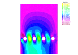
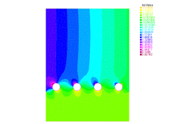
Figure 5: Direct computation $u_{\epsilon,1}$ (left) $u_{\epsilon,2}$ (middle) and $p_{\epsilon}$ (right)

In order to improve accuracy of the direct simulations we use mesh adaptation iterations as described p. 96-97 in [17]: using the hessian matrices of components of ${\bf u}_{\epsilon}$, one defines a metric that modifies the mesh (see fig. 11 (middle) for a final shape of the mesh).

6.2 The microscopic cell problems

Using the same numerical tools, we solve the microscopic problems (14), (15) and (16). These are defined on the infinite perforated strip $Z$: one is forced to truncate the domain and works on $Z_{-L,L}$ with $L>0$ large. We impose boundary data at the top and the bottom of $Z_{-L,L}$ namely

$$\beta_{2}(y)=\Upsilon_{2}(y)=0,\quad\chi_{2}(y)=-1\quad\text{ on }\{y\in]0,1[\times\mathbb{R}\text{ s.t. }y_{2}=\pm L\},$$

and we let natural boundary conditions on the other components. When $L$ goes to infinity it is proved in [23] that the solutions of the truncated problem defined on $Z_{-L,L}$ converge exponentially with respect to $L$ to the solution of the unbounded problem. We compute numerical values of $\overline{\overline{\beta}}_{1}^{\pm}$ and $\overline{\overline{\Upsilon}}_{1}^{\pm}$ and the pressure drop $[\overline{{\overline{\eta}}}]$. If ${\cal J}_{s}$ is a sphere of radius $3/16$ in a period of size 1 centered at $(1/2,1/4)$ the numerical computations provide values listed in table 1.

constants	values	constants	values
$\overline{\overline{\beta}}^{+}_{1}$	-0.377928	$\overline{\overline{\beta}}^{-}_{1}$	-0.122114
$\overline{\overline{\Upsilon}}^{+}_{1}$	-0.000371269	$\overline{\overline{\Upsilon}}^{-}_{1}$	0.121744
$[\overline{{\overline{\eta}}}]$	27.9435

Table 1: Homogenized numerical constants

One can notice that contrary to the resistive matrix of [2] the tangential part of the coefficient are negative. This is due to the fact that the obstacles lie above the interface in the main flow. The horizontal first order slip velocity is thus negative (see below).

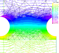
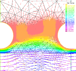
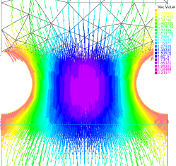
Figure 6: Velocity vectors for micrscopic problems: ${\boldsymbol{\beta}}$ (left), ${\boldsymbol{\Upsilon}}$(middle) and ${\boldsymbol{\chi}}$ (right)

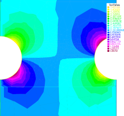
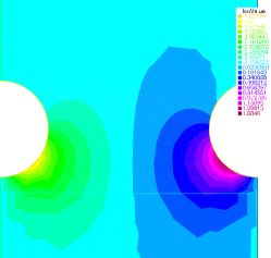
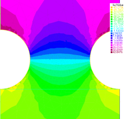
Figure 7: Pressure for micrscopic problems: $\pi$ (left), $\mu$(middle) and $\eta$ (right)

6.3 Explicit first order problem

We solve problem (4) on triangulations of $\Omega_{1}$ and $\Omega_{2}$. Because of the discontinuity of the Dirichlet data at the corners $O$ and $\overline{x}$, the solution $({\bf u}_{1},p_{1})$ does not belong to ${\bf H}^{1}(\Omega_{1}\cup\Omega_{2})\times L^{2}(\Omega_{1}\cup\Omega_{2})$. Indeed a pressure singularity occurs at $O$ and $\overline{x}$: refining the triangulation at the corners one get a point-wise explosion of the pressure near $O$ and $\overline{x}$. We add then the zeroth order explicit poiseuille profile to obtain a numerical approximation of $({\bf\overline{u}}_{\epsilon},\overline{p}_{\epsilon})$. For $\epsilon=0.25$, we display in fig. 8 velocity components and pressure projected on $\Omega_{\epsilon}$ in order to be compared to $({\bf u}_{\epsilon},p_{\epsilon})$ in the next paragraphs.

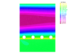
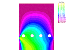
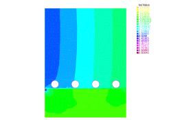
Figure 8: Explicit first order approximation $\overline{u}_{\epsilon,1}$ (left), $\overline{u}_{\epsilon,2}$ (middle) and $\overline{p}_{\epsilon}$ (right)

Since the pressure is not bounded (the numerical value is very high in a very small neighborhood of $O$ and $\overline{x}$ we display the “regular part”: we cut-off the pressure function near the corners for visualisation purposes only.

6.4 Comparisons and error estimates

In fig. 9, we display the horizontal (left) velocity profile above and below the obstacles for the direct solution $\overline{u}_{\epsilon,1}$ and our approximation $\overline{u}_{\epsilon,1}$. In the middle we show the normal velocity in the same framework. On the right of the same figure, we plot various values of $\epsilon$ on the $x$-axis and the flow-rate through ${\Gamma_{0}}$ on the $y$-axis. One observes that the asymptotic expansion gives the first order approximation of the flow-rate with respect to $\epsilon$ near $\epsilon=0$ which was expected. One notices also that the actual rough flow-rate behaves as a square-root of $\epsilon$. This seems difficult to prove using averaged interface conditions only [8, 7].

Figure 9: Velocity profiles for $\epsilon=0.125$ close to ${\Gamma_{0}}$: horizontal (left) and vertical (middle). Rough versus homogenized flow-rates (right) wrt $\epsilon$

In fig. 10, we plot numerical error estimates for the zero order approximation $({\bf u}_{0},p_{0})$ and for our explicit first order averaged approximation $({\bf\overline{u}}_{\epsilon},\overline{p}_{\epsilon})$ wrt to the direct solution $({\bf u}_{\epsilon},p_{\epsilon})$. Left we display the ${\bf L}^{2}(\Omega_{\epsilon})$ error for velocity vectors. On the right, we compute the pressure error estimates in the $H^{-1}(\Omega_{1}^{\prime}\cup{\cal L}_{\epsilon}\cup\Omega_{2})$ norm: for $p_{0}$ (resp. $\overline{p}_{\epsilon}$) we solve numerically

$$\left\{\begin{aligned} &-\Delta q=p_{\epsilon}-p_{0}\,(\text{resp. }\overline{p}_{\epsilon}),&\text{ in }\Omega_{1}^{\prime}\cup{\cal L}_{\epsilon}\cup\Omega_{2},\\ &q=0&\text{ on }\partial\Omega_{1}^{\prime}\cup P\cup\partial\Omega_{2},\end{aligned}\right.$$

for each $\epsilon$ then we display ${\left\|{\nabla q}\right\|}_{L^{2}(\Omega_{1}^{\prime}\cup{\cal L}_{\epsilon}\cup\Omega_{2})}$. One recovers theoretical claims of Theorems 5.1 and 3.1.

Figure 10: Numerical error estimates : velocity (left) and pressure (right) wrt $\epsilon$

In fig. 11 middle and right we display the meshes used for a single value of $\epsilon=0.25$ and for the computations of $({\bf u}_{1},p_{1})$. On the left we display the mesh size $h$ used for the direct simulations with respect to $\epsilon$.

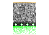
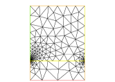
Figure 11: The mesh size $h$ for direct computations (left), a direct mesh for $\epsilon=0.25$ (middle) and the mesh used to compute $({\bf u}_{1},p_{1})$ (right)

Appendix A Well-posedness in weighted Sobolev spaces of the vertical correctors

Given the data $({\bf f},h)$, we study the problem: find $({\bf w},\theta)\in{\mathbf{W}}^{1,2}_{\alpha}(\Pi)\times W^{0,2}_{\alpha}(\Pi)$ solving

$$\left\{\begin{aligned} &-\Delta{\bf w}+\nabla\theta=0&\text{ in }\Pi,\\ &{\rm div\,}{\bf w}=0&\text{ in }\Pi,\\ &{\bf w}={\bf f}&\text{ on }D,\\ &{\bf w}\cdot{\bf\tau}={\bf f}\cdot{\bf\tau},\text{ and }\theta=h&\text{ on }N,\\ \end{aligned}\right.$$ (32)

Remark: 2.

For the specific type of mixed boundary conditions set on $\partial\Pi$, it is not possible to use neither the Fourier transform in the vertical direction nor the Laplace transform in the horizontal direction in order to derive results established below. To our knowledge there are few results in the literature for unbounded domains with mixed boundary conditions on noncompact boundaries.

Theorem A.1.

If the real $\alpha$ is such that $|\alpha|<1$ and if

$${\bf f}\in{\mathbf{W}}^{{\frac{1}{2}},2}_{\alpha}(D\cup N),\quad h\in W^{-{\frac{1}{2}},2}_{\alpha}(N),$$

there exists a unique solution $({\bf w},\theta)\in{\mathbf{W}}^{1,2}_{\alpha}(\Pi)\times W^{0,2}_{\alpha}(\Pi)$ solving problem (32).

Before giving the proof of the theorem, we need to prove two intermediate propositions. For this sake we define

$$\boldsymbol{X}_{\alpha}:=\{{\bf v}\in{\mathbf{W}}^{1,2}_{\alpha}(\Pi)\text{ s.t. }{\bf v}=0\text{ on }D,\quad{\bf v}\cdot{\bf\tau}=0\text{ on }N\},\quad Y_{\alpha}:=W^{0,2}_{\alpha}(\Pi).$$

First we show that the divergence operator is surjective from $\boldsymbol{X}_{\alpha}$ into $Y_{\alpha}$

Proposition 7.

For any given function $q\in Y_{\alpha}$ there exists a vector function ${\bf v}\in\boldsymbol{X}_{\alpha}$ such that

$${\rm div\,}{\bf v}=q,\quad\text{and}\quad{\left|{{\bf v}}\right|}_{\boldsymbol{X}_{\alpha}}\leq k(\Pi,\alpha){\left\|{q}\right\|}_{Y_{\alpha}}$$

where the constant $k$ depends only on the geometry of the domain, and on $\alpha$.

Proof.

We define a sequence of annular domains covering $\Pi$

$$C_{n}:=\{y\in\Pi\text{ s.t. if }y=(r,\tilde{\theta})\text{ then }\quad r\in]2^{n-1},2^{n}[\},\quad n\geq 1,\quad C_{0}:=B(0,1)\cap\Pi.$$

We decompose $q$ as $q=\sum_{n=0}^{\infty}q_{n}$, with $q_{n}:=q\mathbbm{1}_{C_{n}}$. On each $C_{n}$ we solve the problem: find ${\bf v}_{n}\in\boldsymbol{X}_{\alpha,n}$ s.t. ${\rm div\,}{\bf v}_{n}=q_{n}$ and ${\left|{{\bf v}_{n}}\right|}_{\boldsymbol{X}_{\alpha}}\leq k(C_{n},\alpha){\left|{q_{n}}\right|}_{Y_{\alpha}}$, where

$$\boldsymbol{X}_{\alpha,n}:=\left\{{\bf v}\in\boldsymbol{X}_{\alpha}\text{ s.t. }\right. {\bf v}=0\text{ on }\{|y|=2^{n-1}\}\cup\{|y|=2^{n}\}\cup(\overline{C}_{n}\cap D),$$

and $$\left.{\bf v}\cdot{\bf\tau}=0\text{ on }(\overline{C}_{n}\cap N)\right\}.$$

But to solve the latter equation in a weak sense means

$$\int_{C_{n}}{\rm div\,}{\bf v}_{n}\cdot\omega\;rdrd\tilde{\theta}=\int_{C_{n}}q_{n}\cdot\omega\;rdrd\tilde{\theta},\quad\forall\omega\in W^{0,2}_{-\alpha}(C_{n}),$$

making the change of variables: $(\tilde{r}=r/2^{n-1},\tilde{\theta})$ and setting

$$\tilde{{\bf v}}_{n}(\tilde{r},\tilde{\theta}):={\bf v}(2^{n-1}\tilde{r},\tilde{\theta}),\quad\tilde{q}_{n}(\tilde{r},\tilde{\theta}):=q(2^{n-1}\tilde{r},\tilde{\theta}),\quad\tilde{\omega}(\tilde{r},\tilde{\theta}):=\omega(2^{n-1}\tilde{r},\tilde{\theta}),$$

the problem becomes: find $\tilde{{\bf v}}\in\boldsymbol{X}_{0,1}$ defined on $C_{1}$ s.t.

$$\int_{C_{1}}\tilde{{\rm div\,}}\tilde{{\bf v}}_{n}\cdot\tilde{\omega}\tilde{r}d\tilde{r}d\tilde{\theta}=2^{n-1}\int_{C_{1}}\tilde{q}\cdot\tilde{\omega}\;\tilde{r}d\tilde{r}d\tilde{\theta},\quad\forall\omega\in L^{2}(C_{1}),$$

the test space is defined on a compact fixed domain $C_{1}$, weighted Sobolev spaces coincide with the classical ones as soon as the weight is strictly positive and bounded. In this framework the operator $\tilde{{\rm div\,}}:\boldsymbol{X}_{0,1}\to Y_{0,1}$ is surjective thanks to Lemma 4.9 p. 181 in [13]. Thus there exists $\tilde{{\bf v}}_{n}\in\boldsymbol{X}_{0,1}$ s.t. $\tilde{{\rm div\,}}\tilde{{\bf v}}_{n}=\tilde{q}_{n}2^{n-1}$. Note that there is no need of a compatibility condition on the integral of $\tilde{q}_{n}$ as in Lemma 3.1 chap. III in [15] because $\tilde{{\bf v}}_{n}\cdot{\bf n}\neq 0$ on $N\cap\overline{C}_{1}$. Moreover one has that

$${\left|{\tilde{{\bf v}}_{n}}\right|}_{{\bf H}^{1}(C_{1})}\leq k(C_{1},0){\left\|{2^{n-1}\tilde{q}_{n}}\right\|}_{L^{2}(C_{1})},$$

where $k$ depends only on the geometry of $C_{1}$ and is thus independent on $n$. Turning back to the original variables $(r,\tilde{\theta})$ one has then that ${\rm div\,}{\bf v}_{n}=q_{n}$ and

$$\int_{C_{n}}\left|\nabla{\bf v}_{n}\right|^{2}r\,drd\tilde{\theta}\leq k(C_{1},0)\int_{C_{n}}|q_{n}|^{2}r\,drd\tilde{\theta}.$$

In order to recover the global weighted norm of $q$ in $W^{0,2}_{\alpha}(\Pi)$, we multiply the inequality by $2^{2\alpha(n+1)}$ on both sides; we use that for $r\in[2^{n-1},2^{n}]$, $\rho:=(1+r^{2})^{\frac{1}{2}}$ can be estimated as $2^{2\alpha(n-1)}\leq\rho^{2\alpha}\leq 2^{2\alpha(n+1)}$ giving finally

$$\int_{C_{n}}\left|\nabla{\bf v}_{n}\right|^{2}\rho^{2\alpha}dy \leq\int_{C_{n}}\left|\nabla{\bf v}_{n}\right|^{2}2^{2\alpha(n+1)}dy$$

$$\leq k(C_{1},0)2^{2\alpha(n+1)}\int_{C_{n}}q_{n}^{2}dy\leq 2^{4\alpha}k(C_{1},0)\int_{C_{n}}q_{n}^{2}\rho^{2\alpha}dy.$$

One defines ${\bf v}:=\sum_{n}{\bf v}_{n}\mathbbm{1}_{C_{n}}$, because of the boundary conditions imposed on each of the $C_{n}$, ${\bf v}$ is continuous on $\Pi$ and thus belongs to ${\mathbf{W}}^{1,2}_{\alpha}(\Pi)$. This gives the result. ∎

We lift problem (32) by subtracting to ${\bf w}$ a function ${\cal R}({\bf w})$ satisfying:

$${\cal R}({\bf w})\in{\mathbf{W}}^{1,2}_{\alpha}(\Pi),\quad{\cal R}({\bf w})={\bf f}\text{ on }D\cup N.$$

Such a lift exists (cf p. 249 [16] for an explicit form of ${\cal R}({\bf w})$). We correct the divergence of ${\cal R}({\bf w})$ by setting :

$${\cal S}({\bf w})\in\boldsymbol{X}_{\alpha}\text{ s.t. }{\rm div\,}{\cal S}({\bf w})=-{\rm div\,}({\cal R}({\bf w}))\text{ and }{\left\|{{\cal S}({\bf w})}\right\|}_{{\mathbf{W}}^{1,2}_{\alpha}(\Pi)}\leq k{\left\|{{\cal R}({\bf w})}\right\|}_{{\mathbf{W}}^{1,2}_{\alpha}(\Pi)},$$

which is possible thanks to Proposition 7. The new variables $(\tilde{{\bf w}}:={\bf w}-{\cal R}({\bf w})-{\cal S}({\bf w}),\theta)$ solve the homogeneous problem:

$$\left\{\begin{aligned} &-\Delta\tilde{{\bf w}}+\nabla\theta=\Delta{\cal R}({\bf w})+\Delta{\cal S}({\bf w})&\text{ in }\Pi,\\ &{\rm div\,}\tilde{{\bf w}}=0&\text{ in }\Pi,\\ &\tilde{{\bf w}}=0&\text{ on }D,\\ &\tilde{{\bf w}}\cdot{\bf\tau}=0,\text{ and }\theta=h&\text{ on }N.\\ \end{aligned}\right.$$ (33)

No we claim that $({\mathbb{F}},{\mathbb{G}}):=(\rho^{\alpha}\tilde{{\bf w}},\rho^{\alpha}\theta)$ solve in an equivalent way the problem: find $({\mathbb{F}},{\mathbb{G}})$ in ${\mathbf{W}}^{1,2}_{0}(\Pi)\times W^{0,2}_{0}(\Pi)$ s.t.

$$\left\{\begin{aligned} &\begin{aligned} &{\cal A}_{\alpha}\,{\mathbb{F}}+{\cal B}_{\alpha}^{T}{\mathbb{G}}=\rho^{\alpha}(\Delta{\cal R}({\bf w})+\Delta{\cal S}({\bf w}))\\ &{\cal B}_{\alpha}\,{\mathbb{F}}\hskip 34.14322pt=0\\ \end{aligned}&\text{ in }\Pi,\\ &{\mathbb{F}}=0&\text{ on }D\\ &\left.\begin{aligned} {\mathbb{F}}\cdot{\bf\tau}=0\\ {\mathbb{G}}=\rho^{\alpha}h\end{aligned}\right\}&\text{ on }N\end{aligned}\right.$$ (34)

where

$${\cal A}_{\alpha}{\mathbb{F}}:=-\Delta{\mathbb{F}}-2\rho^{\alpha}\nabla{\mathbb{F}}\cdot\nabla\frac{1}{\rho^{\alpha}}-\rho^{\alpha}\Delta\frac{1}{\rho^{\alpha}}{\mathbb{F}},\quad\text{ and } {\cal B}_{\alpha}{\mathbb{F}}:={\rm div\,}{\mathbb{F}}+\rho^{\alpha}\nabla\left(\frac{1}{\rho^{\alpha}}\right)\cdot{\mathbb{F}}.$$ (35)

Indeed, $\rho\in C^{\infty}(\Pi)$ thus if $(\tilde{w},\theta)$ solves (33) in the distributionnal sense, then equivalently by its definition the pair $({\mathbb{F}},{\mathbb{G}})$ solves (34) also in the distributionnal sense. Uniqueness is insured thanks to the onto mapping between ${\mathbf{W}}^{1,2}_{\alpha}(\Pi)\times W^{0,2}_{\alpha}(\Pi)$ and ${\mathbf{W}}^{1,2}_{0}(\Pi)\times W^{0,2}_{0}(\Pi)$ (cf Theorem I.3 p. 243 in [16]): if $(\tilde{w},\theta)$ is a unique solution of (33) then so is $({\mathbb{F}},{\mathbb{G}})$ for system (34) and vice versa. The boundary conditions match between both problems by similar onto trace mappings. Note that the rhs in (34) belongs to ${\mathbf{W}}^{-1,2}_{0}(\Pi)$ and the boundary data to $W^{-{\frac{1}{2}},2}_{0}(N)$. We associate to (34) the corresponding variational setting, namely we define:

• the velocity/pressure test space is $\boldsymbol{X}_{0}\times Y_{0}$,

• the bi-continuous (resp continuous) forms $a_{\alpha},b_{\alpha}$ (resp. $l_{\alpha}$) read

  $$\left\{\begin{aligned} &a_{\alpha}({\mathbb{F}},{\mathbb{V}})=(\nabla{\mathbb{F}},\nabla{\mathbb{V}})-2\left(\rho^{\alpha}\nabla{\mathbb{F}}\nabla\left(\frac{1}{\rho^{\alpha}}\right),{\mathbb{V}}\right)-\left(\rho^{\alpha}\Delta\left(\frac{1}{\rho^{\alpha}}\right){\mathbb{F}},{\mathbb{V}}\right),\quad\forall{\mathbb{F}},{\mathbb{V}}\in\boldsymbol{X}_{0},\\ &b_{\alpha}({\mathbb{F}},{\mathbb{Q}})=-\left({\rm div\,}{\mathbb{F}}+\rho^{\alpha}\nabla\left(\frac{1}{\rho^{\alpha}}\right)\cdot{\mathbb{F}},{\mathbb{Q}}\right),\quad\forall{\mathbb{F}}\in\boldsymbol{X}_{0},\forall{\mathbb{Q}}\in Y_{0},\\ &l_{\alpha}({\mathbb{V}})=(\rho^{\alpha}(\Delta{\cal R}({\bf w})+\Delta{\cal S}({\bf w})),{\mathbb{V}})_{\Pi}-(\rho^{\alpha}h,{\mathbb{V}}\cdot{\bf n})_{N},\quad\forall{\mathbb{V}}\in\boldsymbol{X}_{0}.\\ \end{aligned}\right.$$

• the variational problem: the problem (34) can then be restated in an equivalent way: find $({\mathbb{F}},{\mathbb{G}})\in\boldsymbol{X}_{0}\times Y_{0}$ s.t.

  $$\left\{\begin{aligned} &a_{\alpha}({\mathbb{F}},{\mathbb{V}})&+b_{\alpha}({\mathbb{V}},{\mathbb{G}})&=l_{\alpha}({\mathbb{V}})&\forall{\mathbb{V}}\in\boldsymbol{X}_{0},\\ &b_{\alpha}({\mathbb{F}},{\mathbb{Q}})&&=0&\forall{\mathbb{Q}}\in Y_{0}.\end{aligned}\right.$$

We denote by $\tilde{\cal A}_{\alpha}:\boldsymbol{X}_{0}\to\boldsymbol{X}_{0}^{\prime}$ the operator s.t.

$$a_{\alpha}({\mathbb{F}},{\mathbb{V}})=<\tilde{\cal A}_{\alpha}{\mathbb{F}},{\mathbb{V}}>_{\boldsymbol{X}_{0}^{\prime},\boldsymbol{X}_{0}},\quad\forall{\mathbb{V}}\in\boldsymbol{X}_{0}.$$

The well-posedness of problem (34) is equivalent to two conditions (Theorem A.56 p. 474 [13]):

1. $\tilde{P}\tilde{\cal A}_{\alpha}:\ker({\cal B}_{\alpha})\to\ker({\cal B}_{\alpha})^{\prime}$ is an isomorphism

2. ${\cal B}_{\alpha}:\boldsymbol{X}_{0}\to Y_{0}$ is surjective

where $\tilde{P}$ is the restriction of $\tilde{\cal A}_{\alpha}$ to the kernel of ${\cal B}_{\alpha}$. Here we prove that these conditions are actually fulfilled.

Proposition 15.

If $|\alpha|<1$ then $\tilde{\cal A}_{\alpha}$ satisfies condition $(i)$, whereas ${\cal B}_{\alpha}$ satisfies $(ii)$ without any restrictions on $\alpha$

Proof.

We prove at first that condition $(i)$ is satisfied by showing that $a_{\alpha}$ is a coercive bi-linear form. For every vector ${\mathbb{F}}$ in $\boldsymbol{X}_{0}$, one has after integration by parts of the second term in the definition of $a_{\alpha}$:

$$a_{\alpha}({\mathbb{F}},{\mathbb{F}}) =\left(\alpha\frac{(y\cdot{\bf n})}{\rho^{2}}{\mathbb{F}},{\mathbb{F}}\right)_{\partial\Pi}+{\left|{\nabla{\mathbb{F}}}\right|}_{L^{2}(\Pi)}^{2}$$

$$\quad+\int_{\Pi}\alpha\left(-{\rm div\,}\left(\frac{y}{\rho^{2}}\right)+\left(\frac{2}{\rho^{2}}-\frac{(\alpha+2)|y|^{2}}{\rho^{4}}\right)\right){\mathbb{F}}^{2}dy={\left|{\nabla{\mathbb{F}}}\right|}_{L^{2}(\Pi)}^{2}-\alpha^{2}\int_{\Pi}\frac{|y|^{2}}{\rho^{4}}{\mathbb{F}}^{2}dy,$$

note that the boundary term on the first line above vanishes on $N$ because $(y\cdot{\bf n})=0$, though ${\mathbb{F}}_{1}\neq 0$ on this part of the boundary. Note also that this integration by part is justified for functions in $\boldsymbol{X}_{0}$. We use optimal Poincaré-Wirtinger estimates already presented in the proof of Theorem 5.3 p. 20 in [27]:

$$\int_{\Pi}\left|\frac{{\mathbb{F}}|y|}{\rho^{2}}\right|^{2}dy\leq{\left|{\frac{{\mathbb{F}}}{\rho}}\right|}_{{\bf L}^{2}(\Pi)}^{2}\leq{\left|{\nabla{\mathbb{F}}}\right|}_{{\bf L}^{2}(\Pi)}^{2}.$$

Note that these Poincaré-Wirtinger estimates are possible because of the homogeneous Dirichlet conditions on $D$: they give stronger weights than the corresponding logarithmic weighted Hardy estimates available in the whole $\mathbb{R}^{2}$ [3]. Finally one has

$$(\tilde{\cal A}_{\alpha}{\mathbb{F}},{\mathbb{F}})_{\Pi}\geq(1-\alpha^{2}){\left|{\nabla{\mathbb{F}}}\right|}_{L^{2}(\Pi)^{4}},$$

which implies coercivity of the operator if $|\alpha|<1$. Note that this result (also valid in the scalar case) improves Lemma 4.3 in [5]. This is essentially due to the integration by parts performed on the term $(\nabla{\mathbb{F}}y/\rho^{2},{\mathbb{F}})_{\Pi}$ which avoids estimating this term separately from the others.

We focus on the condition $(ii)$. For all $q\in Y_{0}$ we look for ${\mathbb{F}}\in\boldsymbol{X}_{0}$ s.t.

$${\cal B}_{\alpha}{\mathbb{F}}=q,\text{ and }{\left\|{{\mathbb{F}}}\right\|}_{\boldsymbol{X}_{0}}\leq k{\left\|{q}\right\|}_{W^{0,2}_{0}(\Pi)},$$

but this is equivalent to solve

$${\rm div\,}\left(\frac{{\mathbb{F}}}{\rho^{\alpha}}\right)=\frac{q}{\rho^{\alpha}}.$$

If $q\in Y_{0}$ then $q/\rho^{\alpha}\in W^{0,2}_{\alpha}(\Pi)$ and by Proposition 7 there exists ${\bf v}\in\boldsymbol{X}_{\alpha}$ such that

$${\rm div\,}{\bf v}=\frac{q}{\rho^{\alpha}}\text{ and }{\left|{{\bf v}}\right|}_{{\mathbf{W}}^{1,2}_{\alpha}(\Pi)}\leq k(C_{1},\alpha){\left|{\frac{q}{\rho^{\alpha}}}\right|}_{W^{0,2}_{\alpha}(\Pi)}.$$

Set ${\mathbb{F}}:=\rho^{\alpha}{\bf v}$ thanks to the isomorphism between ${\mathbf{W}}^{1,2}_{\alpha}(\Pi)$ and ${\mathbf{W}}^{1,2}_{0}(\Pi)$ there exists a constant s.t.

$${\left|{{\mathbb{F}}}\right|}_{{\mathbf{W}}^{1,2}_{0}(\Pi)}\leq k_{1}{\left|{{\bf v}}\right|}_{{\mathbf{W}}^{1,2}_{\alpha}(\Pi)}\leq k_{1}k(C_{1},\alpha){\left|{\frac{q}{\rho^{\alpha}}}\right|}_{W^{0,2}_{\alpha}(\Pi)}=k^{\prime}{\left|{q}\right|}_{W^{0,2}_{0}(\Pi)}.$$

∎

Proof of Theorem A.1.

Thanks to the equivalence between well-posedness and conditions $(i)$ and $(ii)$ one concludes the existence and uniqueness of a pair $({\mathbb{F}},{\mathbb{G}})$ solving problem (34). Moreover one has the a priori estimates :

$${\left\|{{\mathbb{F}}}\right\|}_{{\mathbf{W}}^{1,2}_{0}(\Pi)}+{\left\|{{\mathbb{G}}}\right\|}_{W^{0,2}_{0}(\Pi)}\leq k^{\prime} \left({\left\|{\rho^{\alpha}\Delta({\cal R}({\bf w})+{\cal S}({\bf w}))}\right\|}_{{\mathbf{W}}^{-1,2}_{0}(\Pi)}+{\left\|{\rho^{\alpha}h}\right\|}_{W^{-{\frac{1}{2}},2}_{0}(N)}\right)$$

they are obtained similarly to those of Theorem 2.34 p. 100 in [13]. The isomorphism between weighted spaces mentioned above and the equivalence of problems (34) and (33) gives existence and uniqueness of $(\tilde{{\bf w}},\theta)$ solving problem (33) and a priori estimates

$${\left\|{\tilde{{\bf w}}}\right\|}_{{\mathbf{W}}^{1,2}_{\alpha}(\Pi)}+{\left\|{\theta}\right\|}_{W^{0,2}_{\alpha}(\Pi)} \leq k^{\prime\prime}\left\{{\left\|{\Delta({\cal R}({\bf w})+{\cal S}({\bf w}))}\right\|}_{{\mathbf{W}}^{-1,2}_{\alpha}(\Pi)}+{\left\|{h}\right\|}_{W^{-{\frac{1}{2}},2}_{\alpha}(N)}\right\},$$

$$\leq k^{\prime\prime\prime}\left\{{\left\|{{\cal R}({\bf w})+{\cal S}({\bf w})}\right\|}_{{\mathbf{W}}^{1,2}_{\alpha}(\Pi)}+{\left\|{h}\right\|}_{W^{-{\frac{1}{2}},2}_{\alpha}(N)}\right\}.$$

This gives existence and uniqueness of $({\bf w},\theta)$ and due to the continuity of the lifts ${\cal R}({\bf w})$ and ${\cal S}({\bf w})$ with respect to the data, one easily proves that

$${\left\|{{\bf w}}\right\|}_{{\mathbf{W}}^{1,2}_{\alpha}(\Pi)}+{\left\|{\theta}\right\|}_{W^{0,2}_{\alpha}(\Pi)}\leq k^{\prime\prime\prime} \left\{{\left\|{{\bf f}}\right\|}_{{\mathbf{W}}^{{\frac{1}{2}},2}_{\alpha}(D\cup N)}+{\left\|{h}\right\|}_{W^{-{\frac{1}{2}},2}_{\alpha}(N)}\right\}$$

which ends the proof ∎

Proof of Theorem 5.2.

We use Theorem A.1 to prove results for $({\bf w}_{i},\theta_{i})$ for $i\in\{{\boldsymbol{\beta}},{\boldsymbol{\Upsilon}},{\boldsymbol{\chi}},\boldsymbol{\varkappa}\}$. The data for these problems tends exponentially fast to zero: in terms of weights, the Dirichlet (resp Neumann) data is thus compatible with ${\mathbf{W}}^{{\frac{1}{2}},2}_{\alpha}(D)$ (resp. ${\mathbf{W}}^{-{\frac{1}{2}},2}_{\alpha}(N)$) for any real $\alpha$. Setting $\bf{f}=\overline{\overline{{\boldsymbol{\beta}}}}\lambda-{\boldsymbol{\beta}}$ (resp. $\bf{f}=\overline{\overline{\boldsymbol{\Upsilon}}}\lambda-{\boldsymbol{\Upsilon}}$ and $\bf{f}=\overline{\overline{{\boldsymbol{\chi}}}}\lambda-{\boldsymbol{\chi}}$ ) in (32) is equivalent to the first (resp. second and third) problem in (17). Applying Theorem A.1 gives then the claims. ∎

Appendix B Periodic boundary layers: proofs of Propositions 2 and 3 and of Corollary 5.1

of Proposition 2.

We start by lifting the non-homogeneous Dirichlet boundary condition : we set ${\cal R}({\boldsymbol{\beta}}):=y_{2}\phi(y_{2}){\mathbf{e}}_{1}\mathbbm{1}_{Z_{+}}$ and $\tilde{{\boldsymbol{\beta}}}:={\boldsymbol{\beta}}+{\cal R}({\boldsymbol{\beta}})$, this is still a divergence free vector. Now, there exists a unique solution s.t.

$$\left|\nabla\tilde{{\boldsymbol{\beta}}}\right|_{L^{2}(Z)^{4}}\leq\left|\nabla{\cal R}({\boldsymbol{\beta}})\right|_{L^{2}(Z)^{4}}.$$

Indeed, in the space of divergence free $\boldsymbol{D}^{1,2}(Z)$ functions vanishing on $P$, the gradient norm is a norm (via Wirtinger estimates), one proves existence and uniqueness of $\tilde{{\boldsymbol{\beta}}}$ in $\boldsymbol{D}^{1,2}(Z)$ by the Lax-Milgram Theorem.

We apply Lemma 3.4 and Proposition 3.5 of [18] in order to recover the $L^{2}_{{\rm loc}}(Z)$ pressure solving:

$$-\Delta\tilde{{\boldsymbol{\beta}}}+\nabla\pi=-\Delta{\cal R}({\boldsymbol{\beta}}),$$

and this gives existence and uniqueness of $(\tilde{{\boldsymbol{\beta}}},\pi)\in\boldsymbol{D}^{1,2}_{0}(Z)\times L^{2}_{{\rm loc}}(Z)$. On the interface located above (resp. below) the obstacle ${\cal J}_{s}$ we apply the Fourier decomposition in modes as in Theorem 3 p. 10 [24]. One obtains the exponential convergence towards the zero modes of $({\boldsymbol{\beta}},\pi)$ in an explicit way. To derive relationships between constant values at infinity, one has

1. by the divergence free condition that $\overline{\beta}_{2}(\nu)=\overline{\beta}_{2}(\gamma)=0$ for all $\nu\geq y_{2,P}$ and $\gamma\leq 0$.

2. integrating the first equation of (14) in every transverse section $\{y_{2}=\delta\}$ which does not cross the obstacle ${\cal J}_{s}$ gives

   $$\frac{{\rm d}^{2}}{{\rm d}{y_{2}^{2}}}\left(\int_{\{y_{2}=\delta\}}\beta_{1}(y_{1},y_{2})\,dy_{1}\right)=\int_{\{y_{2}=\delta\}}-\frac{\partial^{2}\beta_{1}}{\partial y_{1}^{2}}+\frac{\partial\pi}{\partial y_{1}}\;dy_{1}=0,$$

   by $y_{1}$-periodicity. This implies that $\overline{\beta}(\delta)$ is an affine function of $\delta$. As the gradient rapidly goes to zero, the linear part is zero, we conclude that only the constant remains : thus $\overline{\beta}_{1}(\delta)=\overline{\beta}_{1}(+\infty)$ for $\delta>y_{2,P}$, and $\overline{\beta}_{1}(\nu)=\overline{\beta}_{1}(0)$ for $\nu<0$.

3. Set ${\boldsymbol{G}}:=y_{2}\mathbbm{1}_{Z^{+}}{\mathbf{e}}_{1}$ and $F:=0$, they satisfy:

   $$\left\{\begin{aligned} -&\Delta{\boldsymbol{G}}+\nabla F=-\delta_{\Sigma}{\mathbf{e}}_{1}&\text{ in }Z,\\ &{\rm div\,}{\boldsymbol{G}}=0&\text{ in }Z,\end{aligned}\right.$$ (36)

   we test the first equation in (14) by $G$ and the first equation in (36) by ${\boldsymbol{\beta}}$, then we integrate on $Z_{\nu,\gamma}$ :

   $$(\Delta{\boldsymbol{G}}-\nabla F,{\boldsymbol{\beta}})-(\Delta{\boldsymbol{\beta}}-\nabla\pi,{\boldsymbol{G}})=(\delta_{\Sigma}{\mathbf{e}}_{1},{\boldsymbol{\beta}})=\int_{0}^{1}\beta_{1}(y_{1},0)dy_{1}=\overline{\beta}_{1}(0)$$

   $$=(\sigma_{{\boldsymbol{G}},F}\cdot{\bf n},{\boldsymbol{\beta}})_{\partial Z_{\nu,\gamma}}-(\sigma_{{\boldsymbol{\beta}},\pi}\cdot{\bf n},{\boldsymbol{G}})_{\partial Z_{\nu,\gamma}}=(\sigma_{{\boldsymbol{G}},F}\cdot{\bf n},{\boldsymbol{\beta}})_{P}+\overline{\beta}_{1}(\nu)-(\sigma_{{\boldsymbol{\beta}},\pi}\cdot{\bf n},{\boldsymbol{G}})_{P}$$

   $$=-(\,\partial_{\bf n}\,(y_{2}{\mathbf{e}}_{1}),y_{2}{\mathbf{e}}_{1})_{P}+\overline{\beta}_{1}(\nu)+(\sigma_{{\boldsymbol{\beta}},\pi}\cdot{\bf n},{\boldsymbol{\beta}})_{P}$$

   $$=-(\,\partial_{\bf n}\,(y_{2}{\mathbf{e}}_{1}),y_{2}{\mathbf{e}}_{1})_{P}+\overline{\beta}_{1}(\nu)+{\left|{\nabla{\boldsymbol{\beta}}}\right|}_{L^{2}(Z)},$$

   where we neglected exponentially small terms on $\{y_{2}=\nu\}$ and $\{y_{2}=\gamma\}$. Now we explicit the physical meaning of the constant ${\cal Q}:=(\,\partial_{\bf n}\,(y_{2}{\mathbf{e}}_{1}),y_{2}{\mathbf{e}}_{1})_{P}$

   $${\cal Q}+(\,\partial_{\bf n}\,(y_{2}{\mathbf{e}}_{1}),y_{2}{\mathbf{e}}_{1})_{\{y_{2}=\nu\}\cup\{y_{2}=\gamma\}}=(\Delta(y_{2}{\mathbf{e}}_{1}),y_{2}{\mathbf{e}}_{1})_{Z_{\nu,\gamma}}+|\nabla(y_{2}{\mathbf{e}}_{1})|^{2}_{L^{2}(Z_{\nu,\gamma})^{4}},$$

   which in turn gives :

   $${\cal Q}+\nu-\gamma=\nu-\gamma-|{\cal J}_{s}|,$$

   where $|{\cal J}_{s}|$ is the volume of the obstacle ${\cal J}_{s}$. The quantity $\cal Q$ represents the volume of fluid missing due to the presence of the obstacle ${\cal J}_{s}$ above the limit interface $\Sigma$. If we were to consider a straight channel without a collateral artery but a roughness below the fictitious interface, $\cal Q$ would be a positive number equal to the volume of fluid present below $\Sigma$.

   Computations above are formal and can be rigorously derived by regularizing the obstacle ${\cal J}_{s}$ and then working on regular functions in order to obtain results stated above. None of the final quantities depending on second order derivatives, passing to the limit wrt to the regularization parameter, extends results above to Lipschitz obstacles.

∎

of Proposition 3.

The existence and uniqueness part follows exactly the same lines as in Proposition 2, the exponential convergence is also proved the same way. We detail only relationships between horizontal averages.

• For $\overline{\Upsilon}_{2}$ one uses as for $\overline{\beta}_{2}$ the divergence free condition together with the boundary condition at infinity to obtain that $\overline{\Upsilon}_{2}(y_{2})=0$ for all $y_{2}$ in $\mathbb{R}\setminus]0,y_{2,P}[$.

• Testing the first equation in (15) by ${\boldsymbol{\Upsilon}}$ and integrating on $Z_{\gamma,\nu}$ one gets when passing to the limit wrt $\nu\to\infty,\gamma\to-\infty$ that:

  $$\overline{\Upsilon}_{1}(0)={\left\|{\nabla{\boldsymbol{\Upsilon}}}\right\|}_{L^{2}(Z)}^{2}.$$

  Testing the same equation again but with ${\boldsymbol{G}}=y_{2}{\mathbf{e}}_{1}$ and integrating on $Z_{\nu,\gamma}$ gives:

  $$\overline{\Upsilon}_{1}(\nu)=\overline{\Upsilon}_{1}(\gamma)+(\sigma_{{\boldsymbol{\Upsilon}},\varpi}\cdot{\bf n},y_{2}{\mathbf{e}}_{1})_{P},\quad\forall\nu>y_{2,P},\quad\forall\gamma<0.$$

  We compute:

  $$({\rm div\,}\sigma_{{\boldsymbol{\Upsilon}},\varpi},{\boldsymbol{\beta}})_{Z_{\nu,\gamma}}-({\rm div\,}\sigma_{{\boldsymbol{\beta}},\pi},{\boldsymbol{\Upsilon}})_{Z_{\nu,\gamma}}=-\overline{\beta}_{1}(0)$$

  $$= (\sigma_{{\boldsymbol{\Upsilon}},\varpi}\cdot{\bf n},-y_{2}{\mathbf{e}}_{1})_{P}+(\sigma_{{\boldsymbol{\Upsilon}},\varpi}\cdot{\bf n},{\boldsymbol{\beta}})_{\{y_{2}=\nu\}\cup\{y_{2}=\gamma\}}-(\sigma_{{\boldsymbol{\beta}},\pi}\cdot{\bf n},{\boldsymbol{\Upsilon}})_{\{y_{2}=\nu\}\cup\{y_{2}=\gamma\}}$$

  which gives after passing to the limit wrt $\nu$ and $\gamma$

  $$\overline{\beta}_{1}(0)=(\sigma_{{\boldsymbol{\Upsilon}},\varpi}\cdot{\bf n},y_{2}{\mathbf{e}}_{1})_{P}.$$

• Testing the first equation in (15) against $y_{2}\mathbbm{1}_{Z^{-}}$ and integrating on $Z_{\nu,\gamma}$ one obtains easily that

  $$\overline{\Upsilon}_{1}(y_{2})=\overline{\Upsilon}_{1}(0),\quad\forall y_{2}<0.$$

  Putting together equalities obtained above one concludes the proof.

∎

of Corollary 5.1.

Setting again $\tilde{{\boldsymbol{\beta}}}:={\boldsymbol{\beta}}+y_{2}{\mathbf{e}}_{1}\mathbbm{1}_{Z_{+}}$ and writing

$$(\Delta{\boldsymbol{\chi}}-\nabla\eta,\tilde{{\boldsymbol{\beta}}})_{Z_{\delta,\nu}}+(\Delta{\boldsymbol{\beta}}-\nabla\pi,{\boldsymbol{\chi}})_{Z_{\delta,\nu}}=0$$

$$=(\sigma_{{\boldsymbol{\chi}},\eta}\cdot{\bf n},\tilde{{\boldsymbol{\beta}}})_{\{y_{2}=\delta\}\cup\{y_{2}=\nu\}}-(\sigma_{{\boldsymbol{\beta}},\pi}\cdot{\bf n},{\boldsymbol{\chi}})_{\{y_{2}=\delta\}\cup\{y_{2}=\nu\}}.$$

When passing to the limits $\delta\to\infty$ and $\nu\to-\infty$ in the last expression, one obtains that:

$$-[\overline{\eta\beta_{2}}]^{+\infty}_{-\infty}+[\overline{\pi\chi_{2}}]^{+\infty}_{-\infty}=0,$$

now because $\beta_{2}\to 0$ and $\chi_{2}\to-1$, one gets the desired result at infinity. As the pressure $\pi$ is harmonic in $Z$, the average $\overline{\pi}(\delta)$ is zero in $\mathbb{R}_{-}\cup]y_{2,P},+\infty[$. The same proof holds for $\varpi$. ∎

References

- [1] Y. Achdou, O. Pironneau, and F. Valentin. Effective boundary conditions for laminar flows over periodic rough boundaries. J. Comput. Phys., 147(1):187–218, 1998.
- [2] G. Allaire. Homogenization of the Navier-Stokes equations in open sets perforated with tiny holes. ii. noncritical sizes of the holes for a volume distribution and a surface distribution of holes. Arch. Rational Mech. Anal., 113:261–298, 1991.
- [3] C. Amrouche, V. Girault, and J. Giroire. Weighted sobolev spaces and laplace’s equation in . Journal des Mathematiques Pures et Appliquees, 73:579–606, January 1994.
- [4] L. Augsburger. Flow changes investigation due to the insertion of a braided stent in an inertia driven flow aneurysm model using experimental methods. Technical report, Laboratoire d’Hémodynamique et de Technologie Cardiovasculaire, EPFL, Suisse., 2008.
- [5] E. Bonnetier, D. Bresch, and V. Milisic. A priori convergence estimates for a rough poisson-dirichlet problem with natural vertical boundary conditions. accepted for publication in Advances in Mathematical Fluid Dynamics, 2009.
- [6] A. Bourgeat, O. Gipouloux, and E. Marušić-Paloka. Mathematical modelling and numerical simulation of a non-Newtonian viscous flow through a thin filter. SIAM J. Appl. Math., 62(2):597–626 (electronic), 2001.
- [7] D. Bresch and V. Milisic. High order multi-scale wall laws : part i, the periodic case. accepted for publication in Quart. Appl. Math. 2008.
- [8] D. Bresch and V. Milisic. Towards implicit multi-scale wall laws. accepted for publication in C. R. Acad. Sciences, Série Mathématiques, 2008.
- [9] A. Brillard. Asymptotic flow of a viscous and incompressible fluid through a plane sieve. In Harlow Longman Sci. Tech., editor, Progress in partial differential equations: calculus of variations, applications, volume 267 of Pitman Res. Notes Math., pages 158–172, 1992.
- [10] D. Cioranescu and F. Murat. A strange term coming from nowhere. In Topics in the mathematical modelling of composite materials, volume 31 of Progr. Nonlinear Differential Equations Appl., pages 45–93. Birkhäuser Boston, Boston, MA, 1997.
- [11] C. Conca. Étude d’un fluide traversant une paroi perforée. I. Comportement limite près de la paroi. J. Math. Pures Appl. (9), 66(1):1–43, 1987.
- [12] C. Conca. Étude d’un fluide traversant une paroi perforée. II. Comportement limite loin de la paroi. J. Math. Pures Appl. (9), 66(1):45–70, 1987.
- [13] A. Ern and J.-L. Guermond. Theory and Practice of Finite Elements, volume 159 of Applied Mathematical Series. Springer-Verlag, New York, 2004.
- [14] R. Farwig, G. P. Galdi, and H. Sohr. A new class of weak solutions of the Navier-Stokes equations with nonhomogeneous data. J. Math. Fluid Mech., 8(3):423–444, 2006.
- [15] P.G. Galdi. An introduction to the mathematical theory of the NS equations, vol I & II. Springer, 1994.
- [16] B. Hanouzet. Espaces de Sobolev avec poids application au problème de Dirichlet dans un demi espace. Rend. Sem. Mat. Univ. Padova, 46:227–272, 1971.
- [17] F. Hecht, O. Pironneau, A. Le Hyaric, and Ohtsuka K. Freefem++. Laboratoire Jacques-Louis Lions, Universite Pierre et Marie Curie, Paris, 2005.
- [18] W. Jäger and A. Mikelić. On the boundary conditions at the contact interface between a porous medium and a free fluid. Ann. Scuola Norm. Sup. Pisa Cl. Sci. (4), 23(3):403–465, 1996.
- [19] W. Jäger and A. Mikelic. On the effective equations for a viscous incompressible fluid flow through a filter of finite thickness. Comm. Pure Appl. Math., 1998.
- [20] W. Jäger and A. Mikelić. On the interface boundary condition of Beavers, Joseph, and Saffman. SIAM J. Appl. Math., 60(4):1111–1127, 2000.
- [21] W. Jäger and A. Mikelić. On the roughness-induced effective boundary condition for an incompressible viscous flow. J. Diff. Equa., 170:96–122, 2001.
- [22] W. Jäger and A. Mikelić. Couette flows over a rough boundary and drag reduction. Commun. Math. Phys., 232(3):429–455, 2003.
- [23] W. Jäger, A. Mikelić, and N. Neuss. Asymptotic analysis of the laminar viscous flow over a porous bed. SIAM J. Sci. Comput., 22(6):2006–2028, 2001.
- [24] W. Jäger, A. Mikelić, and N. Neuss. Asymptotic analysis of the laminar viscous flow over a porous bed. Technical report, Simulation in Technology, Interdisciplinary Center for Scientific Computing, Ruprecht-Karls-University, Heidelberg, 2001.
- [25] J.L. Lions and E. Magenes. Non-homogeneous boundary value problems and applications, volume I of Die Grundlehren der mathematischen Wissenschaften. Springer-Verla, 1972.
- [26] T.-M. Liou, S.-N. Liou, and K.-L. Chu. Intra-aneurysmal flow with helix and mesh stent placement across side-wall aneurysm pore of a straight parent vessel. Journal of biomechanical engineering, 126(1):36–43, 2004.
- [27] V. Milisic. Very weak estimates for a rough poisson-dirichlet problem with natural vertical boundary conditions. Methods and Applications of Analysis, 16(2):157–186, June 2009.
- [28] J. Nečas. Les méthodes directes en théorie des équations elliptiques. Masson et Cie, Éditeurs, Paris, 1967.
- [29] N. Neuss, M. Neuss-Radu, and A. Mikelić. Effective laws for the poisson equation on domains with curved oscillating boundaries. Applicable Analysis, 85:479–502, 2006.
- [30] E. Sánchez-Palencia. Nonhomogeneous media and vibration theory, volume 127 of Lecture Notes in Physics. Springer-Verlag, Berlin, 1980.