A Spectral Graph Approach to Discovering Genetic Ancestry

Abstract

Mapping human genetic variation is fundamentally interesting in fields such as anthropology and forensic inference. At the same time patterns of genetic diversity confound efforts to determine the genetic basis of complex disease. Due to technological advances it is now possible to measure hundreds of thousands of genetic variants per individual across the genome. Principal component analysis (PCA) is routinely used to summarize the genetic similarity between subjects. The eigenvectors are interpreted as dimensions of ancestry. We build on this idea using a spectral graph approach. In the process we draw on connections between multidimensional scaling and spectral kernel methods. Our approach, based on a spectral embedding derived from the normalized Laplacian of a graph, can produce more meaningful delineation of ancestry than by using PCA. The method is stable to outliers and can more easily incorporate different similarity measures of genetic data than PCA. We illustrate a new algorithm for genetic clustering and association analysis on a large, genetically heterogeneous sample.

Introduction

Human genetic diversity is of interest in a broad range of contexts, ranging from understanding the genetic basis of disease, to applications in forensic science. Mapping clusters and clines in the pattern of genetic diversity provides the key to uncovering the demographic history of our ancestors. To determine the genetic basis of complex disease, individuals are measured at large numbers of genetic variants across the genome as part of the effort to discover the variants that increase liability to complex diseases such as autism and diabetes.

Genetic variants, called alleles, occur in pairs, one inherited from each parent. High throughput genotyping platforms routinely yield genotypes for hundreds of thousands of variants per sample. These are usually single nucleotide variants (SNPs), which have two possible alleles, hence the genotype for a particular variant can be coded based on allele counts (0,1 or 2) at each variant. The objective is to identify SNPs that either increase the chance of disease, or are physically nearby an SNP that affects disease status.

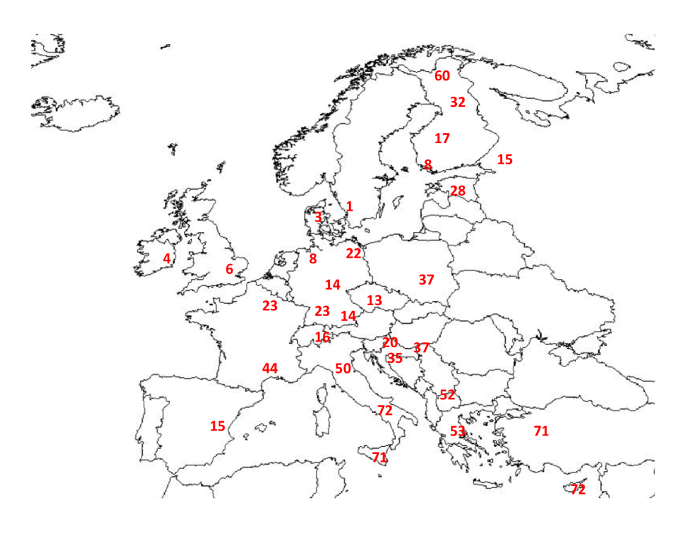
Figure 1: Percent of adult population who are lactose intolerant (http://www.medbio.info/Horn/Time). A gradient runs from north to south, correlating with the spread of the lactase mutation. Finland provides an exception to the gradient due to the Asian influence in the north.

Due to demographic, biological, and random forces, variants differ in allele frequency in populations around the world [Cavalli-Sforza et al., 1994]. An allele that is common in one geographical or ethnic group may be rare in another. For instance, the O blood type is very common among the indigenous populations of Central and South America, while the B blood type is most common in Eastern Europe and Central Asia [Cavalli-Sforza et al., 1994]. The lactase mutation, which facilitates the digestion of milk in adults, occurs with much higher frequency in northwestern Europe than in southeastern Europe (Fig. 1). Ignoring the structure in populations leads to spurious associations in case-control genetic association studies due to differential prevalence of disease by ancestry.

Although most SNPs do not vary dramatically in allele frequency across populations, genetic ancestry can be estimated based on allele counts derived from individuals measured at a large number of SNPs. An approach known as structured association clusters individuals to discrete subpopulations based on allele frequencies [Pritchard et al., 2000]. This approach suffers from two limitations: results are highly dependent on the number of clusters; and realistic populations do not naturally resolve into discrete clusters. If fractional membership in more than one cluster is allowed the calculations becomes computationally intractable for the large data sets currently available. A simple and appealing alternative is principal component analysis (PCA [Cavalli-Sforza et al., 1994; Price et al., 2006; Patterson et al., 2006]), or principal component maps (PC maps). This approach summarizes the genetic similarity between subjects at a large numbers of SNPs using the dominant eigenvectors of a data-based similarity matrix. Using this “spectral” embedding of the data a small number of eigenvectors is usually sufficient to describe the key variation. The PCA framework provides a formal test for the presence of population structure based on the Tracy-Widom distribution [Patterson et al., 2006; Johnstone, 2001]. Based on this theory a test for the number of significant eigenvectors is obtained.

In Europe, eigenvectors displayed in two dimensions often reflect the geographical distribution of populations [Heath et al., 2008; Novembre et al., 2008]. There are some remarkable examples in the population genetics literature of how PC maps can reveal hidden structures in human genetic data that correlate with tolerance of lactose across Europe [Tishkoff et al., 2007], migration patterns and the spread of farming technology from Near East to Europe [Cavalli-Sforza et al., 1994]. Although these stunning patterns can lead to overinterpretation [Novembre and Stephens, 2008], they are remarkably consistent across the literature.

In theory, if the sample consists of $k$ distinct subpopulations, $k-1$ axes should be sufficient to differentiate these subpopulations. In practice, finding a dimension reduction that delineates samples collected worldwide is challenging. For instance, analysis of the four core HapMap samples [African, Chinese, European, and Japanese; HapMap-Consortium, 2005] using the classical principal component map [Patterson et al., 2006] does not reveal substructure within the Asian sample; however, an eigenmap constructed using only the Asian samples discovers substructure [Patterson et al., 2006]. Another feature of PCA is its sensitivity to outliers [Luca et al., 2008]. Due to outliers, numerous dimensions of ancestry appear to model a statistically significant amount of variation in the data, but in actuality they function to separate a single observation from the bulk of the data. This feature can be viewed as a drawback of the PCA method.

Software is available for estimating the significant eigenvectors via PCA (Eigenstrat [Price et al., 2006], smartpca [Patterson et al., 2006], or GEM [Luca et al., 2008]). For population-based genetic association studies, such as case-control studies, the confounding effect of genetic ancestry can be controlled for by regressing out the eigenvectors [Price et al., 2006; Patterson et al., 2006], matching individuals with similar genetic ancestry [Luca et al., 2008; Rosenbaum, 1995], or clustering groups of individuals with similar ancestry and using the Cochran-Mantel-Haenszel test. In each situation, spurious associations are controlled better if the ancestry is successfully modeled.

To overcome some of the challenges encountered in constructing a successful eigenmap of the genetic ancestry, we propose a spectral graph approach. These methods are more flexible than PCA (which can be considered as a special case) and allow for different ways of modeling structure and similarities in data. The basic idea is to represent the population as a weighted graph, where the vertex set is comprised by the subjects in the study, and the weights reflect the degree of similarity between pairs of subjects. The graph is then embedded in a lower-dimensional space using the top eigenvectors of a function of the weight matrix. Our approach utilizes a spectral embedding derived from the so-called normalized graph Laplacian. Laplacian eigenmaps and spectral graph methods are well-known and widely used in machine learning but unfamiliar to many classically trained statisticians and biologists. The goals of this work are to:

• demonstrate the use of spectral graph methods in the analysis of population structure in genetic data

• emphasize the connection between PCA methods used in population genetics and more general spectral methods used in machine learning

• develop a practical algorithm and version of Laplacian eigenmaps for genetic association studies

We proceed by discussing the link between PCA, multidimensional scaling (MDS) and spectral graph methods. We then present a practical scheme for determining the number of significant dimensions of ancestry by studying the gap statistic of the eigenvalues of the graph Laplacian. We conclude with a presentation of the new algorithm, which is illustrated via analyses of the POPRES data [Nelson et al., 2008] and simulated data with spurious associations.

Methods

Spectral embeddings revisited. Connection to MDS and kernel PCA.

We begin by making the connection between multidimensional scaling (MDS) and the principal component (PC) method explicit: Suppose $Z$ is an $n\times p$ data matrix, with rows indexed by $n$ subjects and columns indexed by $p$ biallelic SNP markers. Center each column (marker) to have mean $0$; denote the centered data matrix $X=AZ$ where $A=I-\frac{1}{n}\mathbf{1}\mathbf{1}^{t}$ is an $n\times n$ centering matrix. The elements of the $i$th row of $X$ represent the genetic information for subject $i$, $\mathbf{x}_{i}=(x_{i1},\ldots,x_{ip})$.

A singular value decomposition of $X$ gives

$$X=U\Gamma V^{t},$$

where $\Gamma$ is a diagonal matrix with the singular values $\gamma_{1},\gamma_{2},\ldots$ as diagonal entries. The $p\times p$ matrix

$$S=\frac{1}{n}X^{t}X=\frac{1}{n}V\Gamma^{2}V^{t}$$

is the sample covariance matrix of markers. The eigenvectors $\mathbf{v}_{1},\mathbf{v}_{2}\ldots$ are called principal components. (If the columns of $X$ are furthermore normalized to have standard deviation 1, then $S$ is the sample correlation matrix of markers.) In population genetics, Cavalli-Sforza and others compute the dual $n\times n$ matrix

$$H=XX^{t}=U\Gamma^{2}U^{t},$$

and use the rescaled eigenvectors of $H$ as coordinates of subject $i$,

$$(\lambda_{1}^{1/2}\mathbf{u}_{1}(i),\ldots,\lambda_{d}^{1/2}\mathbf{u}_{d}(i))),$$ (1)

where $\lambda_{j}=\gamma_{j}^{2}$ and $\lambda_{1}\geq\lambda_{2}\geq\ldots$. Geometrically, this corresponds to projecting the data $\mathbf{x}_{i}$ onto the affine hyperplane spanned by the first $d$ principal components, i.e. computing the projection indices or principal component scores $(\mathbf{x}_{i}\cdot\mathbf{v}_{1},\ldots,\mathbf{x}_{i}\cdot\mathbf{v}_{d})$. Typically, eigenvectors that correspond to large eigenvalues reveal the most important dimensions of ancestry.

The matrix $H$ is often referred to as the “covariance matrix of individuals” but this is a bit of a misnomer. In fact, some of the intuition behind the eigenmap method comes from thinking of $H$ as an inner product matrix or Gram matrix. In multivariate statistics, the method of mapping data with principal component scores is known as classical multidimensional scaling. Gower [1966] made explicit the connection between classical MDS and PCA, and demonstrated that the principal components can be extracted from the inner product matrix $H$. The approach is also directly related to kernel PCA [Schölkopf et al., 1998] where all computations are expressed in terms of $H$.

One can show that principal component mapping solves a particular optimization problem with an associated distance metric [Torgerson, 1952; Mardia, 1978]. Refer to the centered data matrix as a feature matrix $X$ where the $i$th row $\mathbf{x}_{i}=(z_{i1}-\bar{z}_{1},\ldots,z_{ip}-\bar{z}_{p})$ is the “feature vector” of the $i$:th individual. In the normalized case, the corresponding vector is $\mathbf{x}_{i}=(\frac{z_{i1}-\bar{z}_{1}}{s_{1}},\ldots,\frac{x_{ip}-\bar{z}_{p}}{s_{p}})$, where $\bar{z}_{j}$ and $s_{j}$, respectively, are the sample mean and sample standard deviation of variable (marker) $j$. The matrix $H$ is a positive semi-definite (PSD) matrix, where element $h_{ij}=\mathbf{x}_{i}\cdot\mathbf{x}_{j}$ reflects the similarity between individuals $i$ and $j$. We will refer to $XX^{t}$ as the kernel of the PC map. The main point is that the matrix $H$ induces a natural Euclidean distance between individuals. We denote this Euclidean distance between the $i^{th}$ and $j^{th}$ individuals as $m(i,j)$, where:

$$m(i,j)^{2}\equiv h_{ii}+h_{jj}-2h_{ij}=\|\mathbf{x}_{i}-\mathbf{x}_{j}\|^{2}.$$ (2)

Consider a low-dimensional representation $\Phi_{d}(i)=(\phi_{1}(i),\ldots,\phi_{d}(i))$ of individuals $i=1,\ldots,n$, where the dimension $d<p$. Define squared distances $\widehat{m}(i,j)^{2}=\|\Phi_{d}(i)-\Phi_{d}(j)\|^{2}$ for this configuration. To measure the discrepancy between the full- and low-dimensional space, let $\delta=\sum_{i,j}(m(i,j)^{2}-\widehat{m}(i,j)^{2})$. This quantity is minimized over all $d$-dimensional configurations by the top $d$ eigenvectors of $H$, weighted by the square root of the eigenvalues (Eq. 1); see Theorem 14.4.1 in [Mardia et al., 1979]. Thus principal component mapping is a form of metric multidimensional scaling. It provides the optimal embedding if the goal is to preserve the squared (pairwise) Euclidean distances $m(i,j)^{2}$ induced by $H=XX^{t}$.

MDS was originally developed by psychometricians to visualize dissimilarity data [Torgerson, 1952]. The downside of using PCA for a quantitative analysis is that the associated metric is highly sensitive to outliers, which diminishes its ability to capture the major dimensions of ancestry. Our goal in this paper is to develop a spectral embedding scheme that is less sensitive to outliers and that is better, in many settings, at clustering observations similar in ancestry. We note that the choice of eigenmap is not unique: Any positive semi-definite matrix $H$ defines a low-dimensional embedding and associated distance metric according to Equations 1 and 2. Hence, we will use the general framework of MDS and principal component maps but introduce a different kernel for improved performance. Below we give some motivation for the modified kernel and describe its main properties from the point of view of spectral graph theory and spectral clustering.

Spectral clustering and Laplacian eigenmaps

Spectral clustering techniques [von Luxburg, 2007] use the spectrum of the similarity matrix of the data to perform dimensionality reduction for clustering in fewer dimensions. These methods are more flexible than clustering algorithms that group data directly in the given coordinate system. Spectral clustering has not been, heretofore, fully explored in the context of a large number of independent genotypes, such as is typically obtained in genome-wide association studies. In the framework of spectral clustering, the decomposition of $XX^{t}$ in PCA corresponds to an un-normalized clustering scheme. Such schemes tend to return embeddings where the principle axes separate outliers from the bulk of the data. On the other hand, an embedding based on a normalized data similarity matrix identifies directions with more balanced clusters.

To introduce the topic, we require the language of graph theory. For a group of $n$ subjects, define a graph $G$ where $\{1,2,\dots,n\}$ is the vertex set (comprised of subjects in the study). The graph $G$ can be associated with a weight matrix $W$, that reflects the strength of the connections between pairs of similar subjects: the higher the value of the entry $w_{ij}$, the stronger the connection between the pair $(i,j)$. Edges that are not connected have weight 0. There is flexibility in the choice of weights and there are many ways one can incorporate application- or data-specific information. The only condition on the matrix W is that it is symmetric with non-negative entries.

Laplacian eigenmaps [Belkin and Niyogi, 2002] find a new representation of the data by decomposing the so-called graph Laplacian — a discrete version of the Laplace operator on a graph. Motivated by MDS, we consider a rescaled parameter-free variation of Laplacian eigenmaps. A similar approach is used in diffusion maps [Coifman et al., 2005] and Euclidean commute time (ECT) maps [Fouss et al., 2007]; both of these methods are MDS-based and lead to Laplacian eigenmaps with rescaled eigenvectors.

The Laplacian matrix $L$ of a weighted graph $G$ is defined by

$$L(i,j)=\left\{\begin{array}[]{l}-w_{ij},\mbox{ if }\>i\neq j,\\ d_{i}-w_{ii},\mbox{ if }i=j,\end{array}\right.$$

where $d_{i}=\sum_{j}w_{ij}$ is the so-called degree of vertex $i$. In matrix form,

$$L=D-W,$$

where $D=diag(d_{1},\dots,d_{n})$ is a diagonal matrix. The normalized graph Laplacian is a matrix defined as

$$\mathcal{L}=D^{-1/2}LD^{-1/2}.$$

A popular choice for weights is $w_{ij}=\exp(-\|\mathbf{x}_{i}-\mathbf{x}_{j}\|^{2}/2\sigma^{2})$, where the parameter $\sigma$ controls the size of local neighborhoods in the graph. Here we instead use a simple transformation of the (global) PCA kernel with no tuning parameters; in Discussion we later suggest a local kernel based on identity-by-state (IBS) sharing for biallelic data. The main point is that one can choose a weight matrix suited for the particular application. Entries in the matrix $XX^{t}$ measure the similarity between subjects, making it a good candidate for a weight matrix on a fully connected graph: the larger the entry for a pair $(i,j)$, the stronger the connection between the subjects within the pair. We define the weights as

$$w_{ij}=\left\{\begin{array}[]{l}\sqrt{\mathbf{x}_{i}\cdot\mathbf{x}_{j}},\mbox{ if }\mathbf{x}_{i}\cdot\mathbf{x}_{j}\geq 0,\\ 0,\mbox{ otherwise.}\end{array}\right.$$

Directly thresholding $XX^{t}$ guarantees non-negative weights but creates a skewed distribution of weights. To address this problem, we have added a square-root transformation for more symmetric weight distributions. This transformation also adds to the robustness to outliers.

Let $\nu_{i}$ and $\mathbf{u}_{i}$ be the eigenvalues and eigenvectors of $\mathcal{L}$. Let $\lambda_{i}=\max\{0,1-\nu_{i}\}$. We replace the PCA kernel $XX^{t}$ with $(I-\mathcal{L})_{+}$, where $I$ is the identity matrix and $(I-\mathcal{L})_{+}\equiv\sum_{i}\lambda_{i}\mathbf{u}_{i}\mathbf{u}_{i}^{t}$ is a positive semi-definite approximation of $I-\mathcal{L}$. We then map the the $i$’th subject into a lower-dimensional space according to Eq. 1. In embeddings, we often do not display the the first eigenvector $\mathbf{u}_{1}$ associated with the eigenvalue $\lambda_{1}=1$, as this vector only reflects the square root of the degrees of the nodes.

In Results, we show that estimating the ancestry from the eigenvectors of $\mathcal{L}$ (which are the same as the eigenvectors of $I-\mathcal{L}$) leads to more meaningful clusters than ancestry estimated directly from $XX^{t}$. Some intuition as to why this is the case can be gained by relating eigenmaps to spectral clustering and “graph cuts”. In graph-theoretic language, the goal of clustering is to find a partition of the graph so that the connections between different groups have low weight and the connections within a group have high weight. For two disjoint sets $A$ and $B$ of a graph, the cut across the groups is defined as $cut(A,B)=\sum_{i\in A,j\in B}w_{ij}$. Finding the partition with the minimum cut is a well-studied problem; however, as noted for example by Shi and Malik [1997] the minimum cut criterion favors separating individual vertices or “outliers” from the rest of the graph. The normalized cut approach by Shi and Malik circumvents this problem by incorporating the volume or weight of the edges of a set into a normalized cost function $Ncut(A,B)=\frac{cut(A,B)}{vol(A)}+\frac{cut(A,B)}{vol(B)},$ where $vol(A)=\sum_{i\in A}d_{i}$ and $vol(B)=\sum_{i\in B}d_{i}$. This cost function is large when the set $A$ or $B$ is small. Our SpectralGEM algorithm (below) exploits the fact that the top eigenvectors of the graph Laplacian provide an approximate solution to the Ncut minimization problem; see Shi and Malik for details. Smartpca [Patterson et al., 2006] and standard GEM [Luca et al., 2008], on the other hand, are biased towards embeddings that favor small and tight clusters in the data.

Number of dimensions via eigengap heuristic

For principal component maps, one can base a formal test for the number of significant dimensions on theoretical results concerning the Tracy-Widom distribution of eigenvalues of a covariance matrix in the null case [Patterson et al., 2006; Johnstone, 2001]. Tracy-Widom theory does not extend to the eigenvalues of the graph Laplacian where matrix elements are correlated. Instead we introduce a different approach, known as the eigengap heuristic, based on the difference in magnitude between successive eigenvalues.

The graph Laplacian has several properties that make it useful for cluster analysis. Both its eigenvalues and eigenvectors reflect the connectivity of the data. Consider, for example, the normalized graph Laplacian where the sample consists of $d$ distinct clusters. Sort the eigenvalues $0=\nu_{1}\leq\nu_{2}\leq\ldots\leq\nu_{n}$ of $\mathcal{L}$ in ascending order. The matrix $\mathcal{L}$ has several key properties [Chung, 1992]: (i) The number $d$ of eigenvalues equal to $0$ is the number of connected components $S_{1},\ldots,S_{d}$ of the graph. (ii) The first positive eigenvalue $\nu_{d+1}$ reflects the cohesiveness of the individual components; the larger the eigenvalue $\nu_{d+1}$ the more cohesive the clusters. (iii) The eigenspace of $0$ (i.e., the vectors corresponding to eigenvalues equal to 0) is spanned by the rescaled indicator vectors $D^{1/2}\mathbf{1}_{S_{k}}$, where $\mathbf{1}_{S_{k}}=1$ if $i\in S_{k}$, and $\mathbf{1}_{S_{k}}=0$ otherwise. It follows from (iii) that for the ideal case where we have $d$ completely separate populations (and the node degrees are similar), individuals from the same population map into the same point in an embedding defined by the $d$ first eigenvectors of $\mathcal{L}$. For example, for $d=3$ populations and $n=6$ individuals, the $n\times d$ embedding matrix could have the form

$$U=[D^{1/2}\mathbf{1}_{S_{1}},\ D^{1/2}\mathbf{1}_{S_{2}},\ D^{1/2}\mathbf{1}_{S_{3}}]=\left(\begin{array}[]{ccc}\sqrt{d_{1}}&0&0\\ \sqrt{d_{2}}&0&0\\ \sqrt{d_{3}}&0&0\\ 0&\sqrt{d_{4}}&0\\ 0&\sqrt{d_{5}}&0\\ 0&0&\sqrt{d_{6}}\par\end{array}\right)\approx\left(\begin{array}[]{ccc}1&0&0\\ 1&0&0\\ 1&0&0\\ 0&1&0\\ 0&1&0\\ 0&0&1\end{array}\right).$$

The rows of $U$ define the new representation of the $n$ individuals. Applying $k$-means to the rows finds the clusters trivially without the additional assumption on the node degrees, if one as in the clustering algorithm by Ng et al. [2001] first re-normalizes the rows of $U$ to norm $1$, or if one according to Shi and Malik [1997] computes eigenvectors of the graph Laplacian $I-D^{-1}W$ instead of the symmetric Laplacian $I-D^{-1/2}WD^{-1/2}$.

In a more realistic situation the between-cluster similarity will rarely be exactly $0$ and all components of the graph will be connected. Nevertheless, if the clusters are distinct, we may still use the eigenvalues of the graph Laplacian to determine the number of significant dimensions. Heuristically, choose the number $d$ of significant eigenvectors such that the eigengaps $\delta_{i}=|\nu_{i+1}-\nu_{i}|$ are small for $i<d$ but the eigengap $\delta_{d}$ is large. One can justify such an approach with an argument from perturbation analysis [Stewart, 1990]. The idea is that the matrix $\mathcal{L}$ for the genetic data is a perturbed version of the ideal matrix for $d$ disconnected clusters. If the perturbation is not too large and the “non-null” eigengap $\delta_{d}$ is large, the subspace spanned by the first $d$ eigenvectors will be close to the subspace defined by the ideal indicator vectors and a spectral clustering algorithm will separate the individual clusters well. The question then becomes: How do we decide whether an eigengap is significant (non-null)?

In this work, we propose a practical scheme for estimating the number of significant eigenvectors for genetic ancestry that is based on the eigengap heuristic and hypothesis testing. By simulation, we generate homogeneous data without population structure and study the distribution of eigengaps for the normalized graph Laplacian. Because there is only one population, the first eigengap $\delta_{1}$ is large. We are interested in the first null eigengap, specifically the difference $\delta_{2}=|\nu_{3}-\nu_{2}|$ between the 2nd and 3rd eigenvalues (note that $\nu_{1}$ is always $0$). If the data are homogeneous, this difference is relatively small. Based on our simulation results, we approximate the upper bound for the null eigengap with the 99th quantile of the sampling distribution as a function of the number of subjects $n$ and the number of SNPs $p$. In the eigenvector representation, we choose the dimension $d$ according to

$$d=\max\{i;\delta_{i}>f(n,p)\},$$

where $f(n,p)=-0.00016+2.7/n+2.3/p$ is the empirical expression for the 99th quantile. For most applications, we have that $p\gg n$ and $f(n,p)\approx 2.7/n$.

Controlling for ancestry in association studies

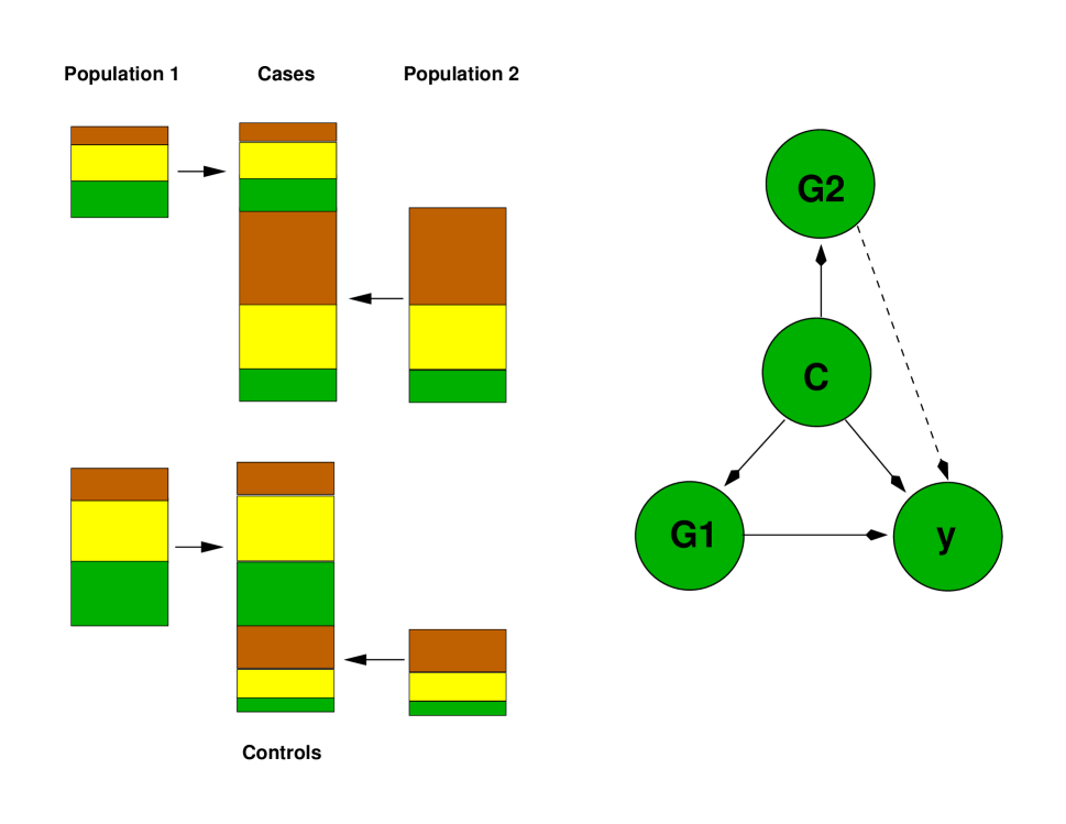
Figure 2: Example of population stratification due to both disease prevalence and allele frequencies varying by ancestry. See text for details.

Due to demographic, biological and random forces, genetic variants differ in allele frequency in populations around the world. A case-control study could be susceptible to population stratification, a form of confounding by ancestry, when such variation is correlated with other unknown risk factors. Fig. 2 shows an example of population stratification. We wish to test the association between candidate SNPs and the outcome (Y) of a disease. In the example, the genotype distributions for Population 1 and 2 are different, as illustrated by the different proportions of red, yellow and green. In addition, there are more cases (Y=1) from Population 2 than 1, and more controls (Y=0) from Population 1 than 2. Let G1 and G2, respectively, be the genotypes of a causal versus a non-causal SNP. The arrow from G1 to Y in the graph to the right indicates a causal association. There is no causal association between G2 and Y but the two variables are indirectly associated, as indicated by the dotted line, through ancestry (C). Ancestry is here a “confounder” as it is both associated with allele frequency and disease prevalence conditional on genotype; it distorts the assessment of the direct relationship between G2 and Y and decreases the power of the study.

Statistical techniques to control spurious findings include stratification by the Cochran-Mantel-Haenszel method, regression and matching Rosenbaum [1995]. These approaches assume that the key confounding factors have been identified, and that at each distinct level of the confounders, the observed genotype is independent of the case and control status. In this work, we estimate confounding ancestry by an eigenanalysis (PCA or spectral graph) of a panel of reference SNPs. Under the additional assumption that the interaction between ancestry and the genotype of the candidate SNPs is neglible, we compare different techniques of controlling for ancestry.

The most straight-forward strategy to correct for stratification is to embed the data using the inferred axes of variation and divide the population into $K$ groups or strata that are homogeneous with respect to ancestry. The Cochran-Mantel-Haenszel (CMH) method represents the data as a series of $K$ contingency tables. One then performs a chi-squared test of the null hypothesis that the disease status is conditionally independent of the genotype in any given stratum. The precision in sample estimates of the CMH test statistic is sensitive to the sample size as well as the balance of the marginals in the contingency table. This can be a problem if we have insufficient data or if cases and controls are sampled from different populations.

An alternative approach is to use a regression model for the disease risk as a function of allele frequency. Effectively, regression models link information from different strata by smoothness assumptions. Suppose that $x$ is the observed allele count (0, 1 or 2) of the candidate SNP, and that the eigenmap coordinates of an individual is given by $\phi_{1},\ldots,\phi_{d}$. Assign $Y=1$ to cases and $Y=0$ to controls and let $q=P(Y=1|x,\phi_{1},\ldots,\phi_{d})$. For a logistic regression model

$$\log\left(\frac{q}{1-q}\right)=\beta x+b_{1}\phi_{1}+\ldots+b_{d}\phi_{d}\ ,$$

the regression parameter $\beta$ can be interpreted as the increase in the log odds of disease risk per unit increase in $x$, holding all other risk variables in the model constant. Thus, the null hypothesis $H_{0}:\beta=0$ is equivalent to independence of disease and SNP genotype after adjusting for ancestry.

A third common strategy to control for confounding is to produce a fine-scale stratification of ancestry by matching. Here we use a matching scheme introduced in an earlier paper [Luca et al., 2008]. The starting point is to estimate ancestry using an eigenanalysis (PCA for “GEM” and the spectral graph approach for “SpectralGEM”). Cases and controls are matched with respect to the Euclidean metric in this coordinate system; hence, the relevance of an MDS interpretation with an explicitly defined metric. Finally, we perform conditional logistic regression for the matched data.

Algorithm for SpectralR and SpectralGEM

Algorithm 1 summarizes the two related avenues that use the spectral graph approach to control for genetic ancestry: SpectralR (for Regression) and SpectralGEM (for GEnetic Matching).

There are many possible variations of the algorithm. In particular, the normalization and rescaling in Steps 3 and 7 can be adapted to the clustering algorithms by Shi-Malik and Ng-Jordan-Weiss. One can also redefine the weight matrix in Step 2 to model different structure in the genetic data.

Algorithm 1 SpectralR and SpectralGEM

1:  Center and scale the allele counts. Let $\mathbf{x}_{i}$ be the genetic information for subject $i$.

2:  Compute weight matrix $W$ where $w_{ij}=(\max\{{\mathbf{x}_{i}\cdot\mathbf{x}_{j}},0\})^{1/2}$.

3:  Compute the normalized Laplacian matrix $\mathcal{L}=I-D^{-1/2}WD^{-1/2}$.

4:  Find the eigenvalues $\nu_{i}$ and eigenvectors $\mathbf{u}_{i}$ of $\mathcal{L}$.

5:  Define the PSD matrix $H=(I-\mathcal{L})_{+}$ with eigenvalues $\lambda_{i}=\max\{0,1-\nu_{i}\}$ and eigenvectors $\mathbf{u}_{i}$. This is the kernel of our map.

6:  Determine the number of significant dimensions $d$ in the eigenvector representation

$$d=\max\{i;\delta_{i}>-0.00016+2.7/n+2.3/p\},$$

7:  Let $\Phi_{d}(i)=(\lambda_{1}^{1/2}\mathbf{u}_{1}(i),\dots,\lambda_{d}^{1/2}\mathbf{u}_{d}(i))$ be the new representation of subject $i$.

8:  For regression (SpectralR):

9:        Perform logistic regression with the the $d$ eigenmap coordinates and the allele count of the candidate SNP as covariates.

10:        Compute p-values for the Wald test of no association between disease and SNP genotype.

11:  For genetic matching (SpectralGEM):

12:        Compute the distance between subjects $i$ and $j$ using $\|\Phi_{d}(i)-\Phi_{d}(j)\|$.

13:        Find homogeneous clusters of individuals via Ward’s $k$-means algorithm [Luca et al., 2008].

14:        Rescale the data as described in the GEM algorithm [Luca et al., 2008].

15:        Remove unmatchable subjects prior to analysis.

16:        Recompute the eigenmap. Match cases and controls in $d$ dimensions.

17:        Perform conditional logistic regression and compute p-values for the Wald test.

Analysis of Data

A large number of subjects participating in multiple studies throughout the world have been assimilated into a freely available database known as POPRES [Nelson et al., 2008]. Data consists of genotypes from a genome-wide 500,000 single-nucleotide polymorphism panel. This project includes subjects of African American, E. Asian, Asian-Indian, Mexican, and European origin. We use these data to assess performance of spectral embeddings. For more detailed analyses of these data see [Lee et al., 2009].

These data are challenging because of the disproportionate representation of individuals of European ancestry combined with individuals from multiple continents. To obtain results more in keeping with knowledge about population demographics, Nelson et al. [2008] supplement POPRES with 207 unrelated subjects from the four core HapMap samples. In addition, to overcome problems due to the dominant number of samples of European ancestry, they remove 889 and 175 individuals from the Swiss and U.K. samples, respectively. Because PCA is sensitive to outliers, they perform a careful search for outliers, exploring various subsets of the data iteratively. After making these adjustments they obtain an excellent description of the ancestry of those individuals in the remaining sample, detecting seven informative axes of variation that highlight important features of the genetic structure of diverse populations. When analysis is restricted to individuals of European ancestry, PCA works very well [Novembre et al., 2008]. Direct application of the approach to the full POPRES data leads to much less useful insights as we show below.

Data Analysis of POPRES

Demographic records in POPRES include the individual’s country of origin and that of his/her parents and grandparents. After quality control the data included 2955 individuals of European ancestry and 346 African Americans, 49 E. Asians, 329 Asian-Indians, and 82 Mexicans. From a sample of nearly 500,000 SNPs we focus on 21,743 SNPs for in depth analysis. These SNPs were chosen because they are not rare (minor allele frequency $\geq.05$), and have a low missingness rate ($\leq.01$). Each pair is separated by at least 10 KB with squared correlation of 0.04 or less.

Outlier Dataset. It is well known that outliers can interfere with discovery of the key eigenvectors and increase the number of significant dimensions discovered with PCA. To illustrate the effect of outliers we created a subsample from POPRES including 580 Europeans (all self-identified Italian and British subjects), 1 African American, 1 E. Asian, 1 Indian and 1 Mexican. Smartpca removes the 4 outliers prior to analysis and discovers 2 significant dimensions of ancestry. If the outliers are retained, 5 dimensions are significant. The first two eigenvectors separate the Italian and British samples and highlight normal variability within these samples. Ancestry vectors 3-5 isolate the outliers from the majority of the data, but otherwise convey little information concerning ancestry.

With SpectralGEM, leaving the outliers in the data has no impact. The method identified 2 significant dimensions that are nearly identical to those discovered by PCA. In our cluster analysis we identified 4 homogeneous clusters: 1 British cluster, 2 Italian clusters, and 1 small cluster that includes the outliers and 6 unusual subjects from the remaining sample.

Cluster Dataset. The ancestral composition of samples for genome-wide association studies can be highly variable. To mimic a typical situation we created a subsample from POPRES including 832 Europeans (all self-identified British, Italian, Spanish and Portuguese subjects), 100 African Americans and 100 Asian-Indians.

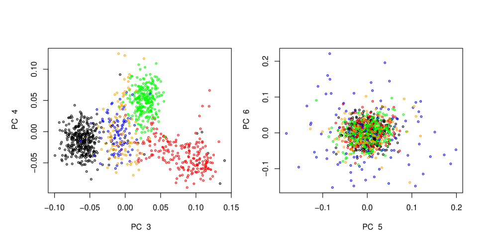
Figure 3: Principal components 3-6 for data from the Cluster Dataset. PC 1 and PC 2 are quite similar to the eigenvectors shown in Fig. 4. Subjects are self-identified as U.K. (black), Italian (red), Iberian Peninsula (green), African American (blue), Indian (orange)

Using smartpca, 7 dimensions of ancestry are significant. The first 2 eigenvectors separate the continental samples. The third and fourth eigenvectors separate the Europeans roughly into three domains ( Fig. 3). The three European populations form three clusters, but they are not completely delineated. The other continental groups generate considerable noise near the center of the plot. The remaining 3 significant dimensions reveal little structure of interest.

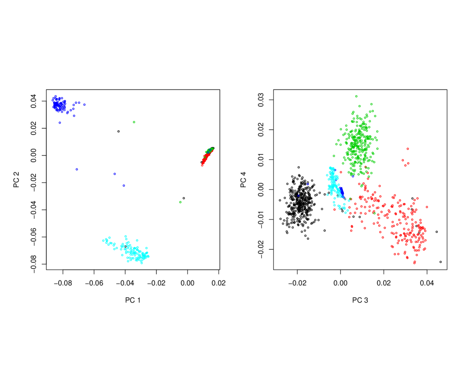
Figure 4: Non-trivial eigenvectors (EV) from the spectral graph approach for the Cluster Dataset. Subjects are self-identified as U.K. (black), Italian (red), Iberian Peninsula (green), African American (blue), Indian (orange).

Using SpectralGEM 4 dimensions are significant (Fig. 4). The first two dimensions separate the continental clusters. In the third and fourth dimensions, the European clusters separate more distinctly than they did for PCA. For these higher dimensions, the samples from other continents plot near to the origin, creating a cleaner picture of ancestry. Six homogeneous clusters are discovered, 3 European clusters, an African American cluster and 2 Indian clusters.

Full Dataset. For the greatest challenge we analyze the full POPRES sample. Smartpca’s 6 standard deviation outlier rule removes 141 outliers, including all of the E. Asian and Mexican samples. If these “outliers” were retained, PCA finds 12 significant dimensions: the first 4 dimensions separate the 5 continental populations (African, European, Latin American, E. Asian and S. Asian). Other eigenvectors are difficult to interpret. Moreover, based on this embedding, Ward’s clustering algorithm failed to converge; thus no sensible clustering by ancestry could be obtained.

With SpectralGEM no outliers are removed prior to analysis. The number of significant dimensions of ancestry is 8. The first 4 dimensions separate the major continental samples; the remaining dimensions separate the European sample into smaller homogeneous clusters.

Applying the clustering algorithm based on this eight dimensional embedding we discover 16 clusters and 3 outliers. Four of these clusters group the African American, E. Asian, Indian and Mexican samples, so that greater than 99% of the subjects in a cluster self-identified as that ancestry, and only a handful of subjects who self-identified as one of those four ancestries fall outside of the appropriate cluster.

The remaining 12 clusters separate the individuals of European ancestry. For ease of interpretation, we removed the samples obtained from Australia, Canada, and the U.S., and focus our validation on 2302 European samples, which can be more successfully categorized by ancestry based on geographic origin. These individuals were classified to one of the 34 European countries represented in the database (Table 1). Sample sizes varied greatly across countries. Seven countries had samples of size 60 or more. Countries with smaller samples were combined to create composite country groupings based on region; see Table 1 for definition of country groupings.

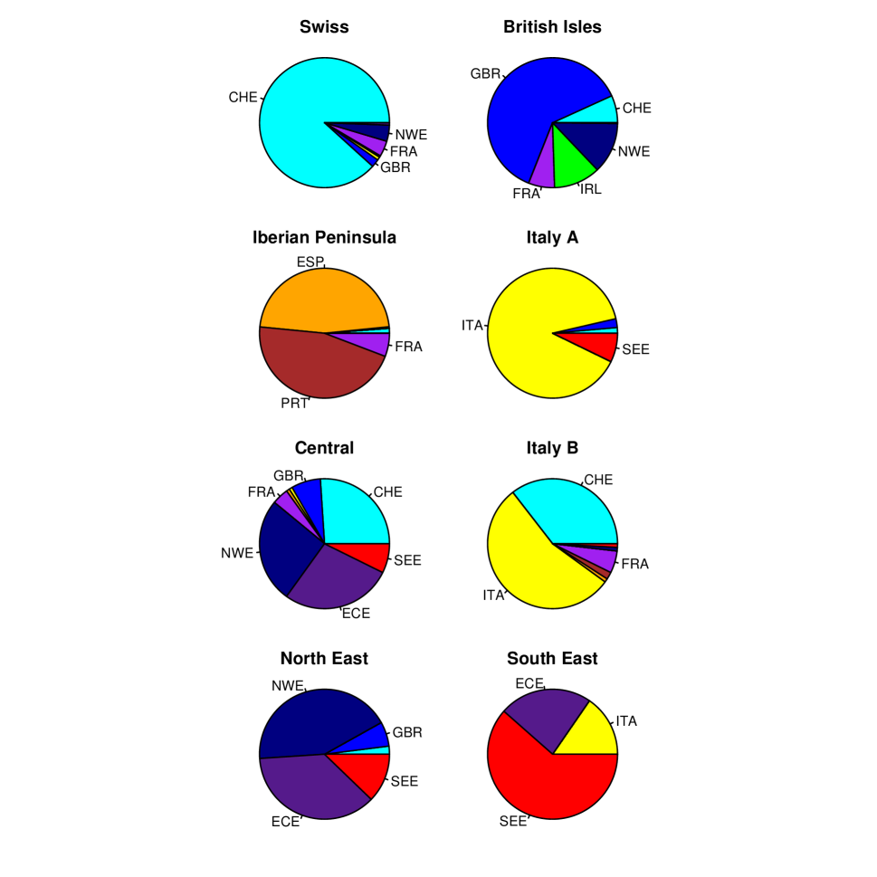
Figure 5: Country membership by cluster for the Full Dataset. Cluster labels and country groupings are defined in Table I. Cluster labels were derived from the majority country or country grouping membership.

By using Ward’s clustering algorithm based on the spectral embedding, all but 81 of the European sample were clustered into one of 8 relatively large European clusters (labeled A-H, Table 1). Fig. 5 illustrates the conditional probability of country grouping given cluster. Clusters tend to consist of individuals sampled from a common ancestry. Labeling the resulting clusters in Fig. 5 by the primary source of their membership highlights the results: (A) Swiss, (B) British Isles, (C) Iberian Peninsula, (D) Italian A, (E) Central, (F) Italian B, (G) North East, and (H) South East. The remaining four small clusters show a diversity of membership and are simply labeled I, J, K, and L. Cluster L has only 7 members who could be classified by European country of origin.

A dendrogram displays the relationships between clusters (Fig. 6). For instance, it appears that the Italian A and B clusters represent Southern and Northern Italy, respectively. Clusters I and J are similar to the Central cluster, while Cluster K represents a more Southern ancestry.

Simulations for association

To compare smartpca with SpectralGEM and SpectralR using the POPRES data it is necessary to create cases ($Y=1$) and controls ($Y=0$) from this undifferentiated sample. Disease prevalence often varies by ancestry due to genetic, environmental and cultural differences. To simulate a realistic case-control sample we wish to mimic this feature. We use cluster membership, $C=k$, $k=1,\ldots,K$, as a proxy for ancestry and assign cases differentially to clusters. In our previous analysis we identified 16 clusters, 12 of European ancestry and 4 of non-European ancestry. For simplicity we reduce the number of European clusters to 8 using the dendrogram and Table 1 to help group the small clusters: K with D, and I, J and L with E.

To generate an association between $Y$ and $C$ we vary $P(Y=1|C=k)$ by cluster. Within each cluster, case and control status is assigned at random. This creates a relationship between $Y$ and the observed SNPs that is purely spurious. Thus we can assess the Type I error rate of smartpca and SpectralGEM to evaluate the efficacy of the two approaches in removing confounding effects induced by ancestry.

To assess power we must generate SNPs associated with $Y$ using a probability model. To maintain as close a correspondence with the observed data as possible, we simulate each causal SNP using the baseline allele frequencies, $p_{k},\,k=1,\ldots,12$, obtained from a randomly chosen SNP in the data base. For cluster $k$, when the individual is a control the simulated genotype is 0, 1 or 2 with probabilities $(1-p_{k})^{2},2p_{k}(1-p_{k})$ or $p_{k}^{2}$, respectively. The association is induced by imposing relative risk $R>1$ which corresponds with the minor allele at a simulated causal locus. Case individuals are assigned genotype 0, 1 and 2 with probabilities proportional to $(1-p_{k})^{2},2Rp_{k}(1-p_{k})$ and $R^{2}p_{k}^{2}$, respectively. We repeat this process to generate $M=1000$ SNPs associated with $Y$.

We wish to compare two approaches for estimating ancestry (PCA and spectral graph) and two approaches for controlling ancestry (regression and matching). Luca et al. (2008) conducted a thorough comparison between regression and matching using eigenvectors derived from PCA. Here we focus on two key comparisons: (i) we control confounding using regression and compare the efficacy of eigenvectors estimated using PCA versus the spectral graph approach (Smartpca versus SpectralR); and (ii) we estimate eigenvectors using the spectral graph approach and compare efficacy of matching versus the regression approach (SpectralGEM versus SpectralR). Finally, we compare all of these methods to the CMH approach which uses the clusters as strata.

We perform the following experiment: randomly sample half of the POPRES data; assign case and control status differentially in clusters according the the model $P(Y|C)$; estimate the eigenvectors using the two approaches based on the $p$ observed SNPs; assess Type I error using the observed SNPs; generate $M$ causal SNPs; assess power using the simulated SNPs. From our previous analysis we know that all of the samples of Indian and Mexican ancestry are declared outliers using the 6 sd rule for outliers. Most practitioners, however, would not discard entire clusters of data. Thus we do not remove outliers in the simulation experiment.

We simulate a disease with differential sampling of cases from each cluster to induce spurious association between $Y$ and the observed genotypes. This experiment is repeated for 5 scenarios (Table 2). In Scenario 1, $P(Y=1|C=k)$ varies strongly by continent, but is approximately constant within Europe. In Scenarios 2 and 3 the tables are reversed, with the variability most exaggerated within Europe. This could occur in practice due to differential efforts to recruit cases in different regions. In Scenarios 3 and 4, $P(Y=1|C=k)$ approximately follows a gradient across Europe with high prevalence in northern Europe and low prevalence in southern Europe. In Scenario 5, $P(Y=1|C)=0$ for three of the small clusters to simulate a situation where some controls were included for convenience, but no cases of corresponding ancestry were included in the study.

All four approaches controlled rates of spurious association fairly well compared to a standard test of association (Table 3). Overall, matching is slightly more conservative than regression (Table 3). For Scenarios 1-4 this leads to a slight excess of control of Type I errors. For Scenario 5, the advantages of matching come to the fore. When regions of the space have either no cases or no controls, the regression approach is essentially extrapolating beyond the range of the data. This leads to an excess of false positives that can be much more dramatic than shown in this simulation in practice [Luca et al., 2008]. The matching approach has to have a minimum of one case and one control per strata, hence it downweights samples that are isolated by pulling them into the closest available strata.

For each scenario the number of significant eigenvectors was 6 or 7 using the spectral graph approach. With PCA the number of dimensions was 16 or 17, i.e the method overestimates the number of important axes of variation. With respect to power, however, there is no penalty for using too many dimensions since the axes are orthogonal. This may explain why the power of smartpca was either equivalent or slightly higher than the power of SpectralR in our simulations. Because matching tends to be conservative, it was also not surprising to find that the power of SpectralR was greater than SpectralGEM. Finally, all of these approaches exhibited greater power than the CMH test, suggesting that control of ancestry is best done at the fine scale level of strata formed by matching cases and controls than by conditioning on the largest homogeneous strata as is done in the CMH test.

Discussion

Mapping human genetic variation has long been a topic of keen interest. Cavalli-Sforza et al. [1994] assimilated data from populations sampled worldwide. From this they created PC maps displaying variation in allele frequencies that dovetailed with existing theories about migration patterns, spread of innovations such as agriculture, and selective sweeps of beneficial mutations. Human genetic diversity is also crucial in determining the genetic basis of complex disease; individuals are measured at large numbers of genetic variants across the genome as part of the effort to discover the variants that increase liability to complex diseases. Large, genetically heterogeneous data sets are routinely analyzed for genome-wide association studies. These samples exhibit complex structure that can lead to spurious associations if differential ancestry is not modeled [Lander and Schork, 1994; Pritchard et al., 2000; Devlin et al., 2001].

While often successful in modelling the structure in data, PCA has some notable weaknesses, as illustrated in our exploration of POPRES [Nelson et al., 2008]. In many settings the proposed spectral graph approach, is more robust and flexible than PCA. Moreover, finding the hidden structure in human populations using a small number of eigenvectors is inherently appealing.

A theory for the eigenvalue distribution of Laplacian matrices, analogous to the Tracy-Widom distribution for covariance matrices, is however not yet available in the literature. Most of current results concern upper and lower bounds for the eigenvalues of the Laplacian [Chung, 1992], the distribution of all eigenvalues of the matrix as a whole for random graphs with given expected degrees [Chung et al., 2003], and rates of convergence and distributional limit theorems for the difference between the spectra of the random graph Laplacian $H_{n}$ and its limit $H$ [Koltchinskii and Giné, 2000; Shawe-Taylor et al., 2002, 2005]. At present, we rely on simulations of homogeneous populations in our work to derive an approximation to the distribution of the key eigengap.

Furthermore, the weight matrix for the spectral graph implemented here was motivated by two features: it is quite similar to the PCA kernel used for ancestry analysis in genetics; and it does not require a tuning parameter. Nevertheless we expect that a local kernel with a tuning parameter could work better. Because the features (SNPs) take on only 3 values, corresponding to three genotypes, the usual Gaussian kernel is not immediately applicable. To circumvent this difficulty, a natural choice that exploits the discrete nature of the data to advantage is based on “IBS sharing”. For individuals $i$ and $j$, let $s_{ij}$ be the fraction of alleles shared by the pair identical by state across the panel of SNPs [Weir, 1996]. Define the corresponding weight as $w_{ij}=\exp\{-(1-s_{ij})^{2}/\sigma^{2}\}$, with tuning parameter $\sigma^{2}$. Preliminary investigations suggest that this kernel can discover the hierarchical clustering structure often found in human populations, such as major continental clusters, each made up of subclusters. Further study is required to develop a data-dependent choice of the tuning parameter.

Acknowledgements. This work was funded by NIH (grant MH057881) and ONR (grant N0014-08-1-0673).

A public domain R language package SpectralGEM is available from the CRAN website, as well as from http://wpicr.wpic.pitt.edu/WPICCompGen/

Country	Subset	Count	Cluster Label
			A	B	C	D	E	F	G	H	I	J	K	L
Switzerland	CHE	1014	871	36	3	2	32	39	1	0	9	14	5	2
England	GBR	26	0	22	0	0	1	0	0	0	1	0	2	0
Scotland	GBR	5	0	5	0	0	0	0	0	0	0	0	0	0
United Kingdom	GBR	344	20	300	0	3	8	0	3	0	1	1	5	1
Italy	ITA	205	8	0	1	124	1	60	0	4	1	2	4	0
Spain	ESP	128	3	0	122	0	1	1	0	0	0	0	1	0
Portugal	PRT	124	1	0	119	0	0	2	0	0	0	0	0	0
France	FRA	108	39	34	15	0	5	6	0	0	3	2	3	1
Ireland	IRL	61	0	61	0	0	0	0	0	0	0	0	0	0
Belgium	NWE	45	21	19	0	0	3	0	0	0	1	1	0	0
Denmark	NWE	1	0	1	0	0	0	0	0	0	0	0	0	0
Finland	NWE	1	0	0	0	0	0	0	1	0	0	0	0	0
Germany	NWE	71	16	22	0	0	22	1	3	0	3	0	2	2
Latvia	NWE	1	0	0	0	0	0	0	1	0	0	0	0	0
Luxembourg	NWE	1	0	0	0	0	1	0	0	0	0	0	0	0
Netherlands	NWE	19	3	15	0	0	1	0	0	0	0	0	0	0
Norway	NWE	2	0	2	0	0	0	0	0	0	0	0	0	0
Poland	NWE	21	0	1	0	0	3	0	16	0	1	0	0	0
Sweden	NWE	10	0	7	0	0	2	0	0	0	0	1	0	0
Austria	ECE	13	3	1	0	0	6	0	0	0	2	0	0	1
Croatia	ECE	8	0	0	0	0	5	0	2	1	0	0	0	0
Czech	ECE	10	1	0	0	0	6	0	3	0	0	0	0	0
Hungary	ECE	18	0	0	0	0	10	0	4	1	2	1	0	0
Romania	ECE	13	0	0	0	0	5	0	2	4	1	1	0	0
Russia	ECE	7	1	0	0	0	0	0	6	0	0	0	0	0
Serbia	ECE	3	0	0	0	0	0	0	1	0	2	0	0	0
Slovenia	ECE	2	0	0	0	0	2	0	0	0	0	0	0	0
Ukraine	ECE	1	1	0	0	0	0	0	0	0	0	0	0	0
Albania	SEE	2	0	0	0	1	0	0	0	1	0	0	0	0
Bosnia	SEE	7	0	0	0	0	3	0	4	0	0	0	0	0
Cyprus	SEE	4	0	0	0	4	0	0	0	0	0	0	0	0
Greece	SEE	5	0	0	0	2	0	0	0	3	0	0	0	0
Kosovo	SEE	1	0	0	0	0	0	0	0	1	0	0	0	0
Macedonia	SEE	3	0	0	0	0	0	1	0	2	0	0	0	0
Turkey	SEE	6	0	0	0	2	0	0	0	3	0	0	0	0
Yugoslavia	SEE	17	0	0	0	1	6	0	2	6	0	2	0	0
Total		2302	988	526	260	139	123	110	49	26	27	25	22	7

Table 1. Counts of Subjects from Each Country Classified to Each Cluster. Labels in column two create country groupings where necessary due to small counts of subjects in many individual countries. Country groupings NWE, ECE, and SEE include countries from north west, east central, and south east Europe, respectively. Eight clusters (A-H) were given descriptive cluster labels based on the majority country or country grouping membership: (A) Swiss, (B) British Isles, (C) Iberian Peninsula, (D) Italian A, (E) Central, (F) Italian B, (G) North East, and (H) South East. The remaining 4 clusters are labeled I, J, K and L.

cluster name	P(cluster)	P(case $|$ cluster)
		Scenario 1	Scenario 2	Scenario 3	Scenario 4	Scenario 5
African-American	0.13	0.33	0.48	0.26	0.25	0.33
Asian Indian	0.13	0.67	0.49	0.27	0.2	0.67
Mexican	0.03	0.2	0.51	0.27	0.34	0.2
Asian	0.02	0.8	0.51	0.26	0.51	0.8
Swiss	0.3	0.5	0.6	0.65	0.62	0.6
British Isles	0.17	0.5	0.8	0.9	0.9	0.85
Iberian Peninsula	0.07	0.51	0.05	0.2	0.45	0
Italian A	0.05	0.5	0.05	0.15	0.1	0
Central European	0.04	0.5	0.39	0.39	0.39	0.2
Italian B	0.04	0.51	0.21	0.6	0.6	0.41
North East European	0.01	0.5	0.21	0.46	0.39	0.21
South East European	0.01	0.62	0.29	0.24	0.19	0

Table 2.

	0.05	0.01	0.005
Scenario 1
No Correction	0.1708	0.0701	0.0477
Smartpca	0.0494	0.0095	0.0049
SpectralR	0.0522	0.0104	0.0052
SpectralGEM	0.0486	0.0091	0.0044
CMH	0.0441	0.0083	0.0041
Scenario 2
No Correction	0.0774	0.0198	0.0112
Smartpca	0.0524	0.0102	0.0051
SpectralR	0.0519	0.0102	0.0050
SpectralGEM	0.0505	0.0096	0.0047
CMH	0.0446	0.0087	0.0042
Scenario 3
No Correction	0.4305	0.2949	0.2507
Smartpca	0.0514	0.0103	0.0049
SpectralR	0.0511	0.0097	0.0051
SpectralGEM	0.0491	0.0096	0.0046
CMH	0.0438	0.0084	0.0040
Scenario 4
No Correction	0.4353	0.2998	0.2564
Smartpca	0.0517	0.0104	0.0051
SpectralR	0.0507	0.0101	0.0052
SpectralGEM	0.0497	0.0097	0.0049
CMH	0.0444	0.0086	0.0044
Scenario 5
No Correction	0.2170	0.1015	0.0734
Smartpca	0.0528	0.0107	0.0053
SpectralR	0.0524	0.0103	0.0051
SpectralGEM	0.0502	0.0096	0.0046
CMH	0.0434	0.0084	0.0042

Table 3. Type I error.

	Scenario 1	Scenario 2	Scenario 3	Scenario 4	Scenario 5
No Correction	0.817	0.832	0.769	0.766	0.815
Smartpca	0.829	0.808	0.785	0.784	0.798
SpectralR	0.832	0.804	0.780	0.782	0.790
SpectralGEM	0.816	0.775	0.757	0.754	0.764
CMH	0.818	0.751	0.741	0.745	0.717

Table 4. Power.

Figure 6: Dendrogram for European clusters from the Full Dataset.

References

- Belkin and Niyogi [2002] Belkin, M. and P. Niyogi (2002). Laplacian eigenmaps and spectral techniques for embedding and clustering. Advances in Neural Information Processing Systems 14.
- Cavalli-Sforza et al. [1994] Cavalli-Sforza, L., P. Menozzi, and A. Piazza (1994). The history and geography of human genes. Princeton: Princeton University Press.
- Chung [1992] Chung, F. (1992). Spectral graph theory. CBMS Regional Conference Series in Mathematics 92.
- Chung et al. [2003] Chung, F., L. Lu, and V. Vu (2003). Spectra of random graphs with given expected degrees. Proceedings of the National Academy of Sciences 100(11), 6313–6318.
- Coifman et al. [2005] Coifman, R., S. Lafon, A. Lee, M. Maggioni, B. Nadler, F. Warner, and S. Zucker (2005). Geometric diffusions as a tool for harmonics analysis and structure definition of data: Diffusion maps. Proceedings of the National Academy of Sciences 102(21), 7426–7431.
- Devlin et al. [2001] Devlin, B., K. Roeder, and L. Wasserman (2001). Genomic control, a new approach to genetic-based association studies. Theor Popul Biol 60, 155–166.
- Fouss et al. [2007] Fouss, F., A. Pirotte, J.-M. Renders, and M. Saerens (2007). Random-walk computation of similarities between nodes of a graph, with application to collaborative recommendation. IEEE Transactions on Knowledge and Data Engineering 19(3), 355–369.
- Gower [1966] Gower, J. C. (1966). Some distance properties of latent root and vector methods in multivariate analysis. Biometrika 53, 325–338.
- Heath et al. [2008] Heath, S. C., I. G. Gut, P. Brennan, J. D. McKay, V. Bencko, E. Fabianova, L. Foretova, M. Georges, V. Janout, M. Kabesch, H. E. Krokan, M. B. Elvestad, J. Lissowska, D. Mates, P. Rudnai, F. Skorpen, S. Schreiber, J. M. Soria, A. C. Syvänen, P. Meneton, S. Herçberg, P. Galan, N. Szeszenia-Dabrowska, D. Zaridze, E. Génin, L. R. Cardon, and M. Lathrop (2008). Investigation of the fine structure of european populations with applications to disease association studies. European Journal of Human Genetics 16, 1413–1429.
- Johnstone [2001] Johnstone, I. (2001). On the distribution of the largest eigenvalue in principal components analysis. Annals of Statistics 29, 295–327.
- Koltchinskii and Giné [2000] Koltchinskii, V. and E. Giné (2000). Random matrix approximation of spectra of integral operators. Bernoulli 6(1), 113–167.
- Lander and Schork [1994] Lander, E. S. and N. Schork (1994). Genetic dissection of complex traits. Science 265, 2037–2048.
- Lee et al. [2009] Lee, A. B., D. Luca, L. Klei, B. Devlin, and K. Roeder (2009). Discovering genetic ancestry using spectral graph theory. Genetic Epidemiology 00(0), 000–000.
- Luca et al. [2008] Luca, D., S. Ringquist, L. Klei, A. Lee, C. Gieger, H. E. Wichmann, S. Schreiber, M. Krawczak, Y. Lu, A. Styche, B. Devlin, K. Roeder, and M. Trucco (2008). On the use of general control samples for genome-wide association studies: Genetic matching highlights causal variants. American Journal of Human Genetics 82(2), 453–463.
- Mardia et al. [1979] Mardia, K., J. Kent, and J. Bibby (1979). Multivariate Analysis. New York: Academic Press.
- Mardia [1978] Mardia, K. V. (1978). Some properties of classical multi-dimensional scaling. Communications in Statistics – Theory and Methods A7, 1233–1241.
- Nelson et al. [2008] Nelson, M. R., K. Bryc, K. S. King, A. Indap, A. Boyko, J. Novembre, L. P. Briley, Y. Maruyama, D. M. Waterworth, G. Waeber, P. Vollenweider, J. R. Oksenberg, S. L. Hauser, H. A. Stirnadel, J. S. Kooner, J. C. Chambers, B. Jones, V. Mooser, C. D. Bustamante, A. D. Roses, D. K. Burns, M. G. Ehm, and E. H. Lai (2008). The population reference sample, popres: A resource for population, disease, and pharmacological genetics research. American Journal of Human Genetics 83(3)(3), 347–358.
- Ng et al. [2001] Ng, A. Y., M. I. Jordan, and Y. Weiss (2001). On spectral clustering: Analysis and an algorithm. Advances in Neural Information Processing Systems 14, 849–856.
- Novembre et al. [2008] Novembre, J., T. Johnson, K. Bryc, Z. Kutalik, A. R. Boyko, A. Auton, A. Indap, K. S. King, S. Bergmann, M. R. Nelson, M. Stephens, and C. D. Bustamante (2008). Genes mirror geography within europe. Nature 456, 98–101.
- Novembre and Stephens [2008] Novembre, J. and M. Stephens (2008). Interpreting principal component analyses of spatial population genetic variation. Nat Genet 40, 646–649.
- Patterson et al. [2006] Patterson, N. J., A. L. Price, and D. Reich (2006). Population structure and eigenanalysis. PLos genetics 2(12)(12), e190 doi:10.1371/journal.pgen.0020190.
- Price et al. [2006] Price, A. L., N. J. Patterson, R. M. Plenge, M. E. Weinblatt, N. A. Shadick, and D. Reich (2006). Principal components analysis corrects for stratification in genome-wide association studies. Nature Genetics 38, 904–909.
- Pritchard et al. [2000] Pritchard, J. K., M. Stephens, and P. Donnelly (2000). Inference of population structure using multilocus genotype data. Genetics 155, 945–959.
- Pritchard et al. [2000] Pritchard, J. K., M. Stephens, N. A. Rosenberg, and P. Donnelly (2000). Association mapping in structured populations. Am J Hum Genet 67, 170–181.
- Rosenbaum [1995] Rosenbaum, P. (1995). Observational Studies. New York: Springer-Verlag.
- Schölkopf et al. [1998] Schölkopf, B., A. Smola, and K.-R. Müller (1998). Nonlinear component analysis as a kernel eigenvalue problem. Neural Computation 10(5), 1299–1319.
- Shawe-Taylor et al. [2002] Shawe-Taylor, J., N. Cristianini, and J. Kandola (2002). On the concentration of spectral properties. In Advances in Neural Information Processing Systems, Volume 14. MIT Press.
- Shawe-Taylor et al. [2005] Shawe-Taylor, J., C. Williams, N. Cristianini, and J. Kandola (2005). On the eigenspectrum of the Gram matrix and the generalisation error of kernel PCA. IEEE Transactions on Information Theory 51(7), 2510–2522.
- Shi and Malik [1997] Shi, J. and J. Malik (1997). Normalized cuts and image segmentation. IEEE Conference on Computer Vision and Pattern Recognition, 731–737.
- Stewart [1990] Stewart, G. (1990). Matrix perturbation theory. Boston: Academic Press.
- Tishkoff et al. [2007] Tishkoff, S. A., F. A. Reed, A. Ranciaro, B. F. Voight, C. C. Babbitt, J. S. Silverman, K. Powell, H. M. Mortensen, J. B. Hirbo, M. Osman, M. Ibrahim, S. A. Omar, T. B. Lema, G. Nyambo, J. Ghori, S. Bumpstead, J. Pritchard, G. A. Wray, and P. Deloukas (2007). Convergent adaptation of human lactase persistence in africa and europe. Nat Genet 39, 31–40.
- Torgerson [1952] Torgerson, W. S. (1952). Multidimensional scaling: I. theory and method. Psychometrika 17, 401–419.
- von Luxburg [2007] von Luxburg, U. (2007). A tutorial on spectral clustering. Statistics and Computing 17(4)(4), 395–416.
- Weir [1996] Weir, B. (1996). Genetic Data Analysis. Sunderland, MA: Sinauer Associates, Inc.