Power Allocation Strategies and Lattice Based Coding schemes for Bi-directional relaying

Abstract

We consider a communication system where two transmitters wish to exchange information through a half-duplex relay in the middle. The channels between the transmitters and the relay have asymmetric channel gains. More specifically, the channels are assumed to be synchronized with complex inputs and complex fading coefficients with an average power constraint on the inputs to the channels. The noise at the receivers have the same power spectral density and are assumed to be white and Gaussian. We restrict our attention to transmission schemes where information from the two nodes are simultaneously sent to the relay during a medium access phase followed by a broadcast phase where the relay broadcasts information to both the nodes. An upper bound on the capacity for the two phase protocol under a sum power constraint on the transmit power from all the nodes is obtained as a solution to a convex optimization problem. We show that a scheme using channel inversion with lattice decoding can obtain a rate a small constant $0.09$ bits from the upper bound at high signal-to-noise ratios. Numerical results show that the proposed scheme can perform very close to the upper bound.

I Introduction

In our previous work [3], we studied the bi-directional relay problem where two users exchange information with each other through a relay in the middle. Therein we assumed same channel gains between the nodes and the relay. In this work we look at a more practical scenario with asymmetric channel gains. There has been recent work on the bi-directional relay problem with asymmetric channel gains. In [1], several schemes including compress and forward, amplify and forward, decode and forward and mixed forward have been suggested. In our work, we show the benefit of using nested lattices for this problem. There has been some work on using nested lattices for asymmetric channel gains in [5, 6]. In [6], a scheme that is optimal at high signal-to-noise ratios (snr) is given for a given realization of the asymmetric channel.

In this paper, we consider a scenario of a fading channel with $L$ channel realizations and assume that channel gains are known to all the nodes. The transmit power is adapted as a function of the channel gains. We show that an upper bound to the achievable exchange capacity (defined later) can be obtained as the solution to a convex optimization problem. We also show that symmetric nested lattices with an appropriate power allocation policy can perform close to the upper bound at high SNRs.

II System Model and Problem Statement

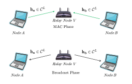
Figure 1: Problem setup with fading links $h_{a}$ and $h_{b}$

We study a simple 3-node linear Gaussian network, with asymmetric channel gains as shown in Fig. 1. Node $A$ and node $B$ wish to exchange information between each other through the relay node $R$. However, nodes $A$ and $B$ cannot communicate with each other directly. The nodes are assumed to be half-duplex, i.e. a node can not transmit and listen at the same time. We use the block fading model to model the channels between the nodes and the relay. The channel gains between the nodes and the relays remain constant over a coherence time interval. It is assumed that the transmission happens over $L$ such coherence time intervals. Each coherence interval corresponds to $N$ uses of the channel. Hence, effectively $NL$ uses of the channel are available for communication. For the channel between the node $A$ and the relay $R$, each of the coefficients of the $L$ length vector $\mathbf{h_{ar}}\in\mathbb{C}^{L}$, represent the channel gain for each coherence time interval. Similarly the channel between the node $B$ and the relay $R$, the relay $R$ and node $A$ and the relay $R$ and node $B$ are captured by the channel gain vectors $\mathbf{h_{br}}$, $\mathbf{h_{ra}}$ and $\mathbf{h_{rb}}\in\mathbb{C}^{L}$ respectively(vectors are denoted by bold face letters such as $\mathbf{v}$ throughout the paper). The channels are assumed to be reciprocal, i.e., $\mathbf{h_{ar}}=\mathbf{h_{ra}}:=\mathbf{h_{a}}$ and $\mathbf{h_{br}}=\mathbf{h_{rb}}:=\mathbf{h_{b}}$.

Let $\mathbf{u}_{A}\in\{0,1\}^{k_{a}L}$ and $\mathbf{u}_{B}\in\{0,1\}^{k_{b}L}$ be the information vectors at nodes $A$ and $B$. We assume a protocol where the communication takes place in two phases at each coherence time interval $i$ ( $i\in\{1,2\ldots L\}$). The phases are the multiple access (MAC) phase and the broadcast phase. $\Delta\in[0,1]$ is the fraction of channel uses for which the MAC phase is used and $(1-\Delta)$ is the fraction of channel uses for which the broadcast phase is used. It is assumed that communication in the MAC and broadcast phases are orthogonal. For example, this could be in two separate frequency bands (or in two different time slots) and hence the MAC phase and broadcast phase do not interfere with each other.

MAC phase

During the MAC phase of each coherence time interval $i$, nodes $A$ and $B$ transmit while the relay node listens. $\mathbf{x_{ai}}\in\mathbb{C}^{\Delta N}$ and $\mathbf{x_{bi}}\in\mathbb{C}^{\Delta N}$ are the transmitted vectors at nodes $A$ and $B$, respectively. The MAC phase takes place in $\Delta N$ uses of the complex additive white Gaussian Channel (AWGN) channel. Further it is assumed that the two transmissions are perfectly synchronized. Hence the received signal at the relay $\mathbf{y_{ri}}\in\mathbb{C}^{\Delta N}$, is given by

$$\mathbf{y_{ri}}=h_{ai}\mathbf{x_{ai}}+h_{bi}\mathbf{x_{bi}}+\mathbf{z_{ri}}$$

where the components of $\mathbf{z_{ri}}\in\mathbb{C}^{\Delta N}$ are independent identically distributed (i.i.d) complex, circularly symmetric Gaussian random variables with zero mean and unit variance. The average transmit power at the nodes $A$ and $B$ in the $i^{th}$ coherence time interval is given as $E[||X_{ai}||^{2}]=P_{ai}$ and $E[||X_{bi}||^{2}]=P_{bi}$.

Broadcast phase

During the broadcast phase, the relay node transmits $\mathbf{x_{ri}}\in\mathbb{C}^{(1-\Delta)N}$ in the $i^{th}$ coherence time interval to both nodes $A$ and $B$. The nodes A and B receive $\mathbf{y_{ai}}$ and $\mathbf{y_{bi}}$, respectively where

$$\mathbf{y_{ai}} = h_{ai}\mathbf{x_{ai}}+\mathbf{z_{ai}}$$

$$\mathbf{y_{bi}} = h_{bi}\mathbf{x_{bi}}+\mathbf{z_{bi}}$$

The average transmit power at the relay node during the $i^{th}$ coherence time interval is given by $P_{ri}$, and the receiver noise at the two nodes is complex Gaussian with zero mean and unit variance.

Further, it is assumed that there is a total sum power constraint over all the nodes. Since the MAC phase is used during the fraction $\Delta$ and the broadcast phase is used during the fraction $(1-\Delta)$ of the available time slots, the total power constraint is expressed as

$$\frac{\Delta}{L}\sum_{i=1}^{L}P_{ai}+\frac{\Delta}{L}\sum_{i=1}^{L}P_{bi}+\frac{(1-\Delta)}{L}\sum_{i=1}^{L}P_{ri}\leq P.$$

We are interested in power allocation strategies and good encoding/decoding schemes that maximize the amount of information (maximize $k_{a}/(LN)+k_{b}/(LN)$) that can be exchanged reliably (such that the probability of error can be made arbitrarily small in the limit of $N\rightarrow\infty$). We refer to the maximum value of $k_{a}/(LN)+k_{b}/(LN)$ that can be reliably exchanged with a given scheme as the exchange rate for that scheme. The exchange capacity is then the supremum of all such rates over the encoding schemes.

III Main Results and comments

We only consider the case when $\Delta=0.5$, or the MAC and broadcast phase each use the channel half the time. For this case, the main results in this paper are

• An upper bound on the exchange rate is setup as a convex optimization problem.

• A scheme is proposed which at high snrs is away from the upper bound by at most 0.09 bits(see Theorem 3). The scheme uses nested lattice encoding and the transmit power is chosen to be inversely proportional to the channel gains.

IV Upper Bound for the two phase protocol

We can easily obtain an upper bound for the two phase protocol using cut-set arguments and as in [1]. In our problem model the channel remains constant in each coherence time interval. Hence, the channel over $L$ such coherence time intervals can be modeled as a set of $L$ parallel channels. At each coherence time interval $i$, the maximum information rate that can be transmitted from node $A$ to node $B$ is bounded by the minimum of the information capacity from node $A$ to relay node $R$, and relay node $R$ to node $B$. This can be expressed as, $\min\{\Delta C(|h_{ai}|^{2}P_{ai}),(1-\Delta)C(|h_{bi}|^{2}P_{ri})\}$, where $C(x):=\log(1+x)$. Here $\Delta$ is the fraction of time node $A$ transmits and $(1-\Delta)$ is the fraction of time the relay node transmits. Similarly the rate that can be transmitted from node $B$ to node $A$ is bounded by the minimum of the information capacity from node $B$ to relay $R$ and from relay $R$ to node $A$, which can be expressed as $\min\{\Delta C(|h_{bi}|^{2}P_{bi}),(1-\Delta)C(|h_{ai}|^{2}P_{ri})\}$. Hence the total rate that can be transmitted over $L$ such coherence time intervals can be expressed as the sum of the rates at each coherence time interval. Combining the above, the upper bound on the exchange capacity can be expressed as the solution of an optimization problem given by,

maximize $$\frac{1}{L}\sum_{i=1}^{L}\min\{\Delta C(|h_{ai}|^{2}P_{ai}),(1-\Delta)C(|h_{bi}|^{2}P_{ri})\}$$

$$+\frac{1}{L}\sum_{i=1}^{L}\min\{\Delta C(|h_{bi}|^{2}P_{bi}),(1-\Delta)C(|h_{ai}|^{2}P_{ri})\}$$

subject to $$\frac{\Delta}{L}\sum_{i=1}^{L}P_{ai}+\frac{\Delta}{L}\sum_{i=1}^{L}P_{bi}+\frac{(1-\Delta)}{L}\sum_{i=1}^{L}P_{ri}\leq P$$ (1)

$$P_{ai},P_{bi},P_{ri}\geq 0,i\in{1,2\ldots L.}$$

Since $\Delta$ is fixed, we can see that the objective function given above is concave and also the constraints form a convex set. Hence convex optimization techniques can be easily applied to this setup to get the optimal solution for the above convex problem.

Though the problem is convex, it is tough to get analytical results for general snr. However to develop some intuition and for ease of analysis, we obtain the power allocation strategy by solving the optimization problem under the high snr approximation, i.e. $C(x):=\log(x)$. We make this precise in the following theorem.

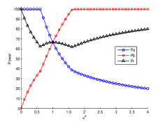
Figure 2: Power allocation as a function of $\kappa^{2}$ for the upper bound

Theorem 1

For finite $L$ and $\Delta=0.5$, and under the high snr approximation, the optimal power allocation for the upper bound on the achievable rate for different ranges of $\kappa_{i}^{2}:=|h_{ai}|^{2}/|h_{bi}|^{2}$ is given by,

Case 1

$0<\kappa_{i}^{2}<=\left.\frac{-1+\sqrt{5}}{2}\right.,$

$$P_{ai}=P\,\,\,\,\,\,P_{bi}=P\frac{\kappa_{i}^{2}}{1+\kappa_{i}^{2}}\,\,\,\,\,\,P_{ri}=P\frac{1}{1+\kappa_{i}^{2}}$$

Case 2

$\left.\frac{-1+\sqrt{5}}{2}\right.<\kappa_{i}^{2}<=\left.\frac{1+\sqrt{5}}{2}\right.,$

$$\begin{split}P_{ai}=P\frac{2}{1+\kappa_{i}^{2}+\kappa_{i}^{4}}\,\,\,\,\,\,P_{bi}=P\frac{2\kappa_{i}^{4}}{1+\kappa_{i}^{2}+\kappa_{i}^{4}}\,\,\,\,\,\,\\ P_{ri}=P\frac{2\kappa_{i}^{2}}{1+\kappa_{i}^{2}+\kappa_{i}^{4}}\end{split}$$

Case 3

$\kappa_{i}^{2}>\left.\frac{1+\sqrt{5}}{2}\right.,$

$$P_{ai}=P\frac{1}{1+\kappa_{i}^{2}}\,\,\,\,\,\,P_{bi}=P\,\,\,\,\,\,P_{ri}=P\frac{\kappa_{i}^{2}}{1+\kappa_{i}^{2}}$$

Proof:

The problem can be solved analytically using the method of Lagrange multipliers and applying the Karush-Kuhn Tucker conditions as given below. The optimization problem for finite $L$ and $\Delta=0.5$ can be expressed below as,

maximize $$\frac{1}{L}\sum_{i=1}^{L}\left(R_{ab}^{(i)}+R_{ba}^{(i)}\right)$$

subject to $$\frac{1}{2}C(|h_{ai}|^{2}P_{ai})>R_{ab}^{(i)},\frac{1}{2}C(|h_{bi}|^{2}P_{ri})>R_{ab}^{(i)}$$

$$\frac{1}{2}C(|h_{bi}|^{2}P_{bi})>R_{ba}^{(i)},\frac{1}{2}C(|h_{ai}|^{2}P_{ri})>R_{ba}^{(i)}$$

$$\frac{1}{L}\sum_{i=1}^{L}\left(P_{ai}+P_{bi}+P_{ri}\right)\leq 2P$$

$$P_{ai},P_{bi},P_{ri}\geq 0,i\in\{1,2\ldots L\}$$

We next use the high snr approximation to simplify the analysis. Under the high snr approximation $C(x)\approx\log x$. The Lagrangian can then be expressed as,

$$\begin{split}\mathcal{L}=-\frac{1}{L}\sum_{i=1}^{L}\left(R_{ab}^{(i)}+R_{ba}^{(i)}\right)\\ +\frac{\lambda}{L}\left(\sum_{i=1}^{L}\left(P_{ai}+P_{bi}+P_{ri}\right)-2P\right)\\ +\sum_{i=1}^{L}\mu_{1}^{(i)}(2R_{ab}^{(i)}-\log(|h_{ai}|^{2}P_{ai}))\\ +\sum_{i=1}^{L}\mu_{2}^{(i)}(2R_{ab}^{(i)}-\log(|h_{bi}|^{2}P_{ri}))\\ +\sum_{i=1}^{L}\mu_{3}^{(i)}(2R_{ba}^{(i)}-\log(|h_{bi}|^{2}P_{bi}))\\ +\sum_{i=1}^{L}\mu_{4}^{(i)}(2R_{ba}^{(i)}-\log(|h_{ai}|^{2}P_{ri}))\end{split}$$

Next taking the partial derivative of $\mathcal{L}$ with respect to each variable in $\mathcal{L}$ and equating to zero, gives us the following set of equations.

$$-\frac{1}{L}+2\mu_{1}^{(i)}+2\mu_{2}^{(i)}=0,-\frac{1}{L}+2\mu_{3}^{(i)}+2\mu_{4}^{(i)}=0$$

$$\frac{\lambda}{L}-\frac{\mu_{1}^{(i)}}{P_{ai}}=0,\frac{\lambda}{L}-\frac{\mu_{3}^{(i)}}{P_{bi}}=0,\frac{\lambda}{L}-\frac{\mu_{2}^{(i)}+\mu_{4}^{(i)}}{P_{ri}}=0$$

Solving for $\lambda$ from the above set of equations gives $\lambda=\frac{1}{2P}$. Solving again the above set of equations for $P_{ai}$, $P_{bi}$ and $P_{ri}$ and together with the Karush-Kuhn Tucker(KKT) conditions, gives us the required power allocation as a function of $\kappa_{i}^{2}$. ∎

In the above proof, the parameter $\lambda$ is not a function of the channel gains. This is so, since we have made the high snr approximation. This implies that the total power allocated $P_{ai}+P_{bi}+P_{ri}$, during each coherence time interval remains the same. However, the power in the individual nodes will vary based on the channel gains. From Theorem 1, we can see that in case 1 we have at low $\kappa_{i}^{2}$, $\kappa_{i}^{2}P_{ai}\approx P_{bi}$. In case 3, where $\kappa_{i}^{2}>>1$, $\kappa_{i}^{2}P_{ai}\approx P_{bi}$. Also for case 2, where $\kappa_{i}^{2}\approx 1$, $\kappa_{i}^{2}P_{ai}\approx P_{bi}$. In other words this implies that $|h_{ai}|^{2}P_{ai}\approx|h_{bi}|^{2}P_{bi}$. In the next section, we propose a scheme that makes use of this property to obtain results close to the upper bound.

V Achievable Scheme using channel inversion and lattice coding

In this section we discuss our achievable scheme based on nested lattice decoding by Erez and Zamir[2]. The proposed scheme follows closely the lattice coding scheme discussed in our previous work [3] and in [4]. The main idea in [3], is that suppose each of the nodes $A$, $B$ and the relay $R$, has the same power constraint (say $P_{\Lambda}$), then at high signal to noise ratios, a rate close to the upper bound $C(P_{\Lambda})$ can be exchanged. In other words, the nested lattice coding approach works best when the receiver channel signal strengths from the two nodes are the same.

In our proposed scheme, we enforce $|h_{ai}|^{2}P_{ai}=|h_{bi}|^{2}P_{bi}$ for every $i^{th}$ coherence time interval in the MAC phase. This matches closely with the observation in section IV, where the power allocation profile at the nodes satisfies $|h_{ai}|^{2}P_{ai}\approx|h_{bi}|^{2}P_{bi}$. This means that each node uses a coarse lattice of power $P_{\Lambda i}$, and each node performs a channel inversion at the transmitter, so that the relay receives equal signal strengths from both the nodes. For the broadcast phase, to ensure that the nodes $A$ and $B$ can decode the message from the relay, we enforce that transmit power at the relay is always larger than the transmit power at the nodes, or $P_{ri}\geq P_{ai},P_{bi}$.

First let us explain our achievable scheme in detail for the $i^{th}$ coherence interval with known channel gains $h_{ai}$, $h_{bi}$. We first obtain the power allocation profiles $P_{ai},P_{bi}$ and $P_{ri}$, based on the additional requirements of $|h_{ai}|^{2}P_{ai}=|h_{bi}|^{2}P_{bi}$ and $P_{ri}\geq P_{ai},P_{bi}$. The allocation is discussed in more detail later in the section. Let us next define $P_{\Lambda i}:=|h_{ai}|^{2}P_{ai}=|h_{bi}|^{2}P_{bi}$ and for each coherence time interval $i$, choose a nested lattice structure having a fine lattice $\Lambda_{i}^{f}$ with a coarse lattice $\Lambda_{i}$ nested in it. The second moment per unit dimension of the coarse lattice is $P_{\Lambda i}/2$. Also the channel model considered in this problem setup has complex inputs and complex noise, when compared to the real Gaussian channel model in [3]. The complex channel provides two degrees of freedom. To take advantage of this we can perform nested lattice coding separately along the in-phase and the quadrature phase components. In all the vectors discussed below namely $\mathbf{x_{ai}},\mathbf{x_{bi}},\mathbf{t_{ai}},\mathbf{t_{bi}},\mathbf{u_{ai}}$ and $\mathbf{u_{bi}}$ are complex vectors and can be expressed as the complex sum of their in-phase and quadrature phase components. For example $\mathbf{x_{ai}}$ can be expressed as ${\rm Re}\{\mathbf{x_{ai}}\}+\jmath{\rm Im}\{\mathbf{x_{ai}}\}.$

First at each coherence interval $i$ during the MAC phase, the data at the nodes $A$ and $B$ are mapped to lattice points $\mathbf{t_{ai}}$ and $\mathbf{t_{bi}}$ respectively. Let $\mathbf{u_{ai}}$ and $\mathbf{u_{bi}}$ be dithers that are uniformly distributed over the coarse lattice. The in-phase component of the dither and the quadrature phase component are independent of each other and each distributed uniformly in the coarse lattice $\Lambda_{i}$, with second moment $P_{\Lambda i}$. An output $(\mathbf{t_{ai}}-\mathbf{u_{ai}})\mod\Lambda_{i}$ is obtained at node $A$ and $(\mathbf{t_{bi}}-\mathbf{u_{bi}})\mod\Lambda_{i}$ at node $B$. Here $\mathbf{t_{i}}\mod\Lambda_{i}$ represents $({\rm Re}\{\mathbf{t_{i}}\}\mod\Lambda_{i})+\jmath({\rm Im}\{\mathbf{t_{i}}\}\mod\Lambda_{i})$

Hence the transmitted vector $\mathbf{x_{ai}}$ at node $A$ is given by,

$$\mathbf{x_{ai}}=\frac{(\mathbf{t_{ai}}-\mathbf{u_{ai}})\mod\Lambda_{i}}{h_{ai}}$$ (2)

Here the numerator $(\mathbf{t_{ai}}-\mathbf{u_{ai}})\mod\Lambda_{i}$ is the sum of the in-phase and quadrature phase components, expressed as ${\rm Re}(\mathbf{t_{ai}}-\mathbf{u_{ai}})\mod\Lambda_{i}+\jmath{\rm Im}(\mathbf{t_{ai}}-\mathbf{u_{ai}})\mod\Lambda_{i}$. Hence the second moment of the numerator per unit dimension is $P_{\Lambda i}/2+P_{\Lambda i}/2=P_{\Lambda i}.$ Hence the average transmit power on $\mathbf{x_{ai}}$ is $P_{\Lambda i}/|h_{ai}|^{2}=P_{ai}.$ Thus we meet the average power constraint of $P_{ai}$ at node $A$. Similarly the transmitted vector $\mathbf{x_{bi}}$ at node $B$ is given below. This also meets the average power constraint $P_{bi}$.

$$\mathbf{x_{bi}}=\frac{(\mathbf{t_{bi}}-\mathbf{u_{bi}})\mod\Lambda_{i}}{h_{bi}}$$ (3)

The relay receives

$$\mathbf{y_{ri}}=h_{ai}\mathbf{x_{ai}}+h_{bi}\mathbf{x_{bi}}+\mathbf{z_{ri}}$$ (4)

or

$$\mathbf{y_{ri}}=(\mathbf{t_{ai}}-\mathbf{u_{ai}})\mod\Lambda_{i}+(\mathbf{t_{bi}}-\mathbf{u_{bi}})\mod\Lambda_{i}+\mathbf{z_{ri}}$$ (5)

The decoder next forms $(\mathbf{y_{ri}}+\mathbf{u_{ai}}+\mathbf{u_{bi}})\mod\Lambda_{i}$ and performs nested lattice decoding and decodes to $\mathbf{t_{ri}}=(\mathbf{t_{ai}}+\mathbf{t_{bi}})\mod\Lambda_{i}$ with high probability, as long as the transmission rate from each of the nodes is less than $2\{\frac{1}{2}\log(0.5+P_{\Lambda_{i}})\}$. The factor 2 is present because the channel coefficients are complex and we have 2 degrees of freedom.

The relay next forms $(\mathbf{t_{ri}}-\mathbf{u_{ri}})\mod\Lambda_{i}$ and during the broadcast phase transmits

$$\mathbf{x_{ri}}=\sqrt{\frac{P_{ri}}{P_{\Lambda_{i}}}}\{(\mathbf{t_{ri}-\mathbf{u_{ri}})\mod\Lambda_{i}\}}$$ (6)

The relays can decode to $\mathbf{t_{ri}}$ as $|h_{ai}|^{2}P_{ri},|h_{bi}|^{2}P_{ri}\geq P_{\Lambda_{i}}$, since $P_{ri}\geq P_{ai},P_{bi}$. Hence effectively a rate of $\frac{1}{2}\log(0.5+P_{\Lambda i})$ can be achieved by the nodes.

Also define $D(x):={u.c.e}\{\log(0.5+x),0.5\log(1+2x)\},x\geq 0$. Here $u.c.e$ denotes the upper concave envelope of the two functions. Hence the optimization problem can be expressed as follows with a few more constraints added.

maximize $$\frac{1}{L}\sum_{i=1}^{L}\min\{\Delta D(|h_{ai}|^{2}P_{ai}),(1-\Delta)D(|h_{bi}|^{2}P_{ri})\}$$

$$+\frac{1}{L}\sum_{i=1}^{L}\min\{\Delta D(|h_{bi}|^{2}P_{bi}),(1-\Delta)D(|h_{ai}|^{2}P_{ri})\}$$

subject to $$\frac{\Delta}{L}\sum_{i=1}^{L}P_{ai}+\Delta\sum_{i=1}^{L}P_{bi}+\frac{(1-\Delta)}{L}\sum_{i=1}^{L}P_{ri}\leq P,$$

$$|h_{ai}|^{2}P_{ai}=|h_{bi}|^{2}P_{bi},$$

$$P_{ri}\geq P_{ai},$$

$$P_{ri}\geq P_{bi},$$

$$P_{ai},P_{bi},P_{ri}\geq 0,i\in{1,2\ldots L}$$

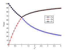
Figure 3: Power allocation as a function of $\kappa^{2}$ for our proposed scheme

The above optimization problem is solved for the case for $\Delta=0.5$ under the high snr assumption with $D(x)$ approximated by $\log(x)$. The next theorem gives us the power allocation profile at the different nodes for different values of $\kappa_{i}^{2}:=|h_{ai}|^{2}/|h_{bi}|^{2}$.

Theorem 2

For finite $L$ with $\Delta=0.5$ and under the high snr approximation, the optimal power allocation for the achievable scheme for different ranges of $\kappa_{i}^{2}:=|h_{ai}|^{2}/|h_{bi}|^{2}$ is given by,

Case 1

$0<\kappa_{i}^{2}<=1,$

$$P_{ai}=P\frac{2}{2+\kappa_{i}^{2}}\,\,\,\,\,\,P_{bi}=P\frac{2\kappa_{i}^{2}}{2+\kappa_{i}^{2}}\,\,\,\,\,\,P_{ri}=P\frac{2}{2+\kappa_{i}^{2}}$$

Case 2

$\kappa_{i}^{2}>1,$

$$P_{ai}=P\frac{2}{1+2\kappa_{i}^{2}}\,\,\,\,\,\,P_{bi}=P\frac{2\kappa_{i}^{2}}{1+2\kappa_{i}^{2}}\,\,\,\,\,\,P_{ri}=P\frac{2\kappa_{i}^{2}}{1+2\kappa_{i}^{2}}$$

Proof:

The problem can be solved analytically using the method of Lagrange multipliers and using the Karush-Kuhn Tucker conditions following along the same lines as in the proof of Theorem 1. ∎

VI Comparison of the upper bound and the achievable schemes

Next we state the main theorem of this paper that compares the upper bound and the achievable scheme for known channel state information in $L$ coherence intervals.

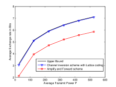
Figure 4: Comparison of bounds for $\Delta=0.5$

Theorem 3

For general $L$ with $\Delta=0.5$, and under the high snr approximation, the achievable rate using the channel inversion scheme with lattice decoding suffers at most a constant $\eta=0.08972$ bits per complex channel use from the upper bound.

Proof:

We compare analytically the results of Theorem 1 and Theorem 2 under the high snr approximation. For different values of $\kappa_{i}$ we compare the exchange rates and we can easily show that the channel inversion scheme suffers at max $0.08972$ bits per complex channel use from the upper bound. ∎

Theorem 3, hence captures the loss due to adding the additional constraints to the upper bound, and the loss is found to be really small. Fig.4 shows some results obtained by numerical solving the optimization problems without the high snr approximation. Here we have $L=100$, and the channel coefficients are taken from a Rayleigh distribution, and they have unit variance. The channel coefficients are fixed and we evaluate the average rate per channel use, each for the upper bound, the lattice based scheme and also the amplify forward scheme.

VII Practical issues with power allocation design

In the previous sections, we discussed techniques to compute the optimal power allocation for a given $\mathbf{h_{a}},\mathbf{h_{b}}$ and $\mathbf{h_{r}}$. However, in practice we are interested in maximizing the average exchange capacity, i.e., the problem is to

maximize $$\mathbb{E}_{h_{a},h_{b}}\left[\min\{\Delta C(|h_{a}|^{2}P_{a}),(1-\Delta)C(|h_{b}|^{2}P_{r})\}\right.$$

$$\left.+\min\{\Delta C(|h_{b}|^{2}P_{b}),(1-\Delta)C(|h_{a}|^{2}P_{r})\}\right]$$

subject to $$\mathbb{E}_{h_{a},h_{b}}\left[\Delta P_{a}+\Delta P_{b}+(1-\Delta)P_{r}\right]\leq P$$

$$P_{a},P_{b},P_{r}\geq 0.$$

Due to the ergodic nature of the channel, the above optimization problem is identical to the one in (1) when $L\rightarrow\infty$. The result in Fig. 4 have been obtained by solving the optimization problem for one realization of $\mathbf{h_{a}},\mathbf{h_{b}}$ and $\mathbf{h_{r}}$ but with $L=100$. Note that while computing the optimal power allocation policy requires us to use a large value of $L$ and optimize the policy, once this policy is fixed, the actual transmit power is chosen based only on the instantaneous channel realization.

VIII Conclusion

In this paper we studied the bi-directional relay problem in which the channels between the nodes and the relays were assumed to have complex inputs with complex fading coefficients. We studied power allocation policies at the nodes for a two phase transmission scheme under the sum transmit power constraint over all nodes. For $\Delta=0.5$, where each phase uses the channel exactly half the time, we obtained an upper bound on the exchange capacity as a solution to a convex optimization problem. We proposed a scheme using nested lattice encoding with the transmit power chosen to be inversely proportional to the channel gains. We obtained analytical solutions for the exchange capacity under the high snr approximation and showed that our proposed scheme can obtain a rate which is at most $0.09$ bits away from the upper bound. For $\Delta\neq 0.5$, we were unable to obtain a good performance using a simple channel inversion power allocation policy. However, it can be shown that using lattice codes with asymmetric rates [6] at the nodes, the upper bound can be achieved at high snrs.

References

- [1] S. J. Kim, N. Devroye, P. Mitran and V. Tarokh, “Achievable rate regions for bi-directional relaying”, arxiv.org 2008.
- [2] U. Erez and R. Zamir, “Achieving on the AWGN channel with lattice encoding and decoding,” IEEE Tran. Info. Theory, vol. 50, pp. 2293 2314, October 2004.
- [3] K. R. Narayanan, M. P. Wilson and A. Sprintson,“Joint Physical Layer Coding and Network Coding for Bi-Directional Relaying”, 45th Annual Allerton Conference on Communication, Control and Computing, September 2007.
- [4] B. Nazer and M. Gastpar, “Lattice Coding Increases Multicast Rates for Gaussian Multiple-Access Networks”, 45th Annual Allerton Conference on Communication, Control and Computing, September 2007.
- [5] I. J. Baik and S. Y. Chung, “Network coding for two-way relay channels using lattices”, Proc. IEEE International Conference on Communications, Beijing, China, May 2008.
- [6] W. Nam, S. Y. Chung and Y. H. Lee, “ Capacity bounds for two-way relay channels”, Proc. IEEE International Zurich Seminar on Communications, Zurich, Switzerland, March 2008.