Linearly Coupled Communication Games

Abstract

This paper discusses a special type of multi-user communication scenario, in which users’ utilities are linearly impacted by their competitors’ actions. First, we explicitly characterize the Nash equilibrium and Pareto boundary of the achievable utility region. Second, the price of anarchy incurred by the non-collaborative Nash strategy is quantified. Third, to improve the performance in the non-cooperative scenarios, we investigate the properties of an alternative solution concept named conjectural equilibrium, in which individual users compensate for their lack of information by forming internal beliefs about their competitors. The global convergence of the best response and Jacobi update dynamics that achieve various conjectural equilibria are analyzed. It is shown that the Pareto boundaries of the investigated linearly coupled games can be sustained as stable conjectural equilibria if the belief functions are properly initialized. The investigated models apply to a variety of realistic applications encountered in the multiple access design, including wireless random access and flow control.

I Introduction

Game theory provides a formal framework for studying the interactions of strategic agents. Recently, there has been a surge in research activities that employ game theory to model and analyze a wide range of application scenarios in modern communication networks [1]-[4]. In communication networks, any action taken by a single user usually affects the utilities of the other users sharing the same resources. Depending on the characteristics of different applications, numerous game-theoretical models and solution concepts have been proposed to describe the multi-user interactions and optimize the users’ decisions in communication networks. Roughly speaking, the existing multi-user research can be categorized into two types, non-cooperative games and cooperative games. Various game theoretic solutions were developed to characterize the resulting performance of the multi-user interaction, including the Nash Equilibrium (NE) and the Pareto-optimality [18].

Non-cooperative approaches generally assume that the participating users simply choose actions to selfishly maximize their individual utility functions. It is well-known that if devices operate in a non-cooperative manner, this will generally limit their performance as well as that of the whole system, because the available resources are not always efficiently exploited due to the conflicts of interest occurring among users [5]. Most non-cooperative approaches are devoted to investigating the existence and properties of the NE. In particular, several non-cooperative game models, such as S-modular games, congestion games, and potential games, have been extensively applied in various communication scenarios [6]-[9]. The price of anarchy, a measure of how good the system performance is when users play selfishly and reach the NE instead of playing to achieve the social optimum, has also been addressed in several communication network applications [10][11].

On the other hand, cooperative approaches in communication theory usually focus on studying how users can jointly improve their performance when they cooperate. For example, the users may optimize a common objective function, which represents the Pareto-optimal social welfare allocation rule based on which the system-wide resource allocation is performed [12][13]. A profile of actions is Pareto-optimal if there is no other profile of actions that makes every player at least as well off and at least one player strictly better off. Allocation rules, e.g. network utility maximization, can provide reasonable allocation outcomes by considering the trade-off between fairness and efficiency. Most cooperative approaches focus on studying how to efficiently find the optimum joint policy. It is worth mentioning that information exchanges among users is generally required to enable users to coordinate in order to achieve and sustain Pareto-efficient outcomes.

In this paper, we present a game model for a particular type of non-cooperative multi-user communication scenario. We name it linearly coupled communication games, because users’ utilities are linearly impacted by their competitors’ actions. In particular, the main contributions of this paper are as follows. First, based on the assumptions that we make about the properties of users’ utility, we characterize the inherent structures of the utility functions for the linearly coupled games. Furthermore, based on the derived utility forms, we explicitly quantify the NE and Pareto boundary for the linearly coupled communication games. The price of anarchy incurred by the selfish users playing the Nash strategy is quantified. In addition, to improve the performance in the non-cooperative scenarios, we investigate an alternative solution: conjectural equilibrium (CE). Using this approach, individual users are modeled as belief-forming agents that develop internal beliefs about their competitors and behave optimally with respect to their individual beliefs. Necessary and sufficient conditions that guarantee the convergence of different dynamic update mechanisms, including the best response and Jacobi update, are addressed. We prove that these adjustment processes based on conjectures and non-cooperative individual optimization can be globally driven to Pareto-optimality in the linearly coupled games without the need of real-time coordination information exchange among agents.

The rest of this paper is organized as follows. Section II defines the linearly coupled communication games. For the investigated game models, Section III explicitly computes the NE and Pareto boundary of the achievable utility region and quantifies the price of anarchy. Section IV introduces the CE and investigates its properties under both the best response and Jacobi update dynamics. Conclusions are drawn in Section V.

II Game Model

In this section, we first provide a general game-theoretic formulation of the multi-user interaction in communication systems. Following the proposed definition, we define the linearly coupled communication games and provide concrete examples of the investigated game model.

II-A Linearly Coupled Communication Games

The multi-user game in various communication scenarios can be formally defined as a tuple $\Gamma=\langle\mathcal{N},\mathcal{A},u,\mathcal{S},s\rangle$. In particular, $\mathcal{N}=\{1,2,\ldots,N\}$ is the set of communication devices, which are the rational decision-makers in the system. Define $\mathcal{A}$ to be the joint action space $\mathcal{A}=\times_{n\in\mathcal{N}}\mathcal{A}_{n}$, with $\mathcal{A}_{n}$ being the action set available for user $n$. As opposed to the traditional strategic game definition[18], we introduce two new elements $\mathcal{S}$ and $s$ into the game formulation. Specifically, $\mathcal{S}$ is the state space $\mathcal{S}=\times_{n\in\mathcal{N}}\mathcal{S}_{n}$, where $\mathcal{S}_{n}\subseteq\mathcal{R}_{+}$ is the part of the state relevant to user $n$. The state is defined to capture the effects of the multi-user coupling such that each user’s utility solely depends on its own state and action. In other words, the utility function $u=\times_{n\in\mathcal{N}}u_{n}$ is a mapping from the individual users’ state space and action space to real numbers, $u_{n}:\mathcal{S}_{n}\times\mathcal{A}_{n}\rightarrow\mathcal{R}$. The state determination function $s=\times_{n\in\mathcal{N}}s_{n}$ maps joint actions to states for each component $s_{n}:\mathcal{A}\rightarrow\mathcal{S}_{n}$. To capture the performance tradeoff, the utility region is defined as $\mathcal{U}=\{(u_{1}(\textbf{a}),\ldots,u_{N}(\textbf{a}))|\ \exists\ \textbf{a}=(a_{1},a_{2},\ldots,a_{N})\in\mathcal{A}\}$.

Definition 1

A multi-user interaction is considered a linearly coupled communication game if the action set $\mathcal{A}_{n}\subseteq\mathcal{R}_{+}$ is convex and the utility function $u_{n}$ satisfies:

$$u_{n}(\mathbf{a})=a_{n}^{\beta_{n}}\cdot s_{n}(\mathbf{a}),$$ (1)

in which $\beta_{n}>0$. In particular, the basic assumptions about $s_{n}(\mathbf{a})$ include:

A1: $s_{n}(\mathbf{a})$ is non-negative;

A2: Denote $s^{\prime}_{nm}(\mathbf{a})=\frac{\partial s_{n}(\mathbf{a})}{\partial a_{m}}$ and $s^{\prime\prime}_{nm}(\mathbf{a})=\frac{\partial^{2}s_{n}(\mathbf{a})}{\partial a_{m}^{2}}$. $s_{n}(\mathbf{a})$ is strictly linear decreasing in $a_{m},\forall m\neq n$, i.e. $s^{\prime}_{nm}(\mathbf{a})<0$ and $s^{\prime\prime}_{nm}(\mathbf{a})=0$; $s_{n}(\mathbf{a})$ is non-increasing and linear in $a_{n}$, i.e. $s^{\prime}_{nn}(\mathbf{a})\leq 0$ and $s^{\prime\prime}_{nn}(\mathbf{a})=0$.

A3: $\frac{s_{n}(\mathbf{a})}{s^{\prime}_{nm}(\mathbf{a})}$ is an affine function, $\forall n\in\mathcal{N}\setminus\{m\}$.

A4: $\frac{s^{\prime}_{nm}(\mathbf{a})}{s_{n}(\mathbf{a})}=\frac{s^{\prime}_{km}(\mathbf{a})}{s_{k}(\mathbf{a})},\forall n,k\in\mathcal{N}\setminus\{m\}$; $\frac{s^{\prime}_{mm}(\mathbf{a})}{s_{m}(\mathbf{a})}=0$ or $\frac{s^{\prime}_{nm}(\mathbf{a})}{s_{n}(\mathbf{a})},\ \forall n\neq m$.

Assumptions A1 and A2 indicate that increasing $a_{m}$ for any $m\neq n$ within the domain of $s_{n}(\mathbf{a})$ will linearly decrease user $n$’s utility. Assumptions A3 and A4 imply that a user’s action has proportionally the same impact over the other users’ utility. The structure of the utility functions that satisfy assumptions A1-A4 will be addressed in Section III.

II-B Illustrative Examples

There are a number of multi-user communication scenarios that can be modeled as linearly coupled communication games. For example, in the random access scenario [15], the action of a node is to select its transmission probability and a node $n$ will independently attempt transmission of a packet with transmit probability $p_{n}$. The action set available to node $n$ is $\mathcal{A}_{n}=[0,1]$ for all $n\in\mathcal{N}$. In this case, the utility function is defined as

$$u_{n}(\mathbf{p})=p_{n}\cdot\prod_{m\neq n}(1-p_{m}).$$ (2)

As an additional example, in flow control [16], $N$ Poisson streams of packets are serviced by a single exponential server with departure rate $\mu$ and each class can adjust its throughput $r_{n}$. The utility function is defined as the weighted ratio of the throughput over the average experienced delay:

$$u_{n}(\mathbf{r})=r_{n}^{\beta_{n}}\cdot(\mu-\sum_{m=1}^{N}r_{m}),$$ (3)

in which $\beta_{n}>0$ is interpreted as the weighting factor. Specifically, we can see that the state determination functions are $s_{n}(\mathbf{p})=\prod_{m\in\mathcal{N}\setminus\{n\}}(1-p_{m})$ in (2) and $s_{n}(\mathbf{r})=\mu-\sum_{m=1}^{N}r_{m}$ in (3). It is straightforward to verify that these functions satisfy assumptions A1-A4 for both (2) and (3).

In this paper, we are interested in comparing the achievable performance attained by different game-theoretic solution concepts. On one hand, it is well-known that NE is generally inefficient in communication games [17], but it may not require explicit message exchanges, while Pareto-optimality can usually be achieved only by exchanging implicit or explicit coordination messages among the participating users. On the other hand, in several recent works [14][15], we have applied an alternative solution in different communication scenarios to improve the system performance in non-cooperative settings, namely the conjectural equilibrium [21]. The following sections aim to compare the solutions of NE, Pareto boundary, and CE in terms of the payoffs and informational requirements in the linearly coupled multi-user interaction satisfying the assumptions A1-A4.

III Computation of the Nash Equilibrium and Pareto Boundary for Linearly Coupled Games

In this section, we show that the computation of the NE and the Pareto boundary in linearly coupled games is equivalent to solving linear equations. Specifically, we investigate the inherent structures of the utility functions satisfying assumptions A1-A4 and define two basic types of linearly coupled games. The performance loss incurred by the Nash strategy are quantified for Type II games.

III-A Nash Equilibrium

In non-cooperative games, the participating users simply choose actions to selfishly maximize their individual utility functions. The steady state outcome of such interactions is an operating point, at which given the other users’ actions, no user can increase its utility alone by unilaterally changing its action. This operating point is known as the Nash equilibrium, which is formally defined below [18].

Definition 2

A profile $\mathbf{a}$ of actions constitutes a Nash equilibrium of $\Gamma$ if $u_{n}(a_{n},\mathbf{a}_{-n})\geq u_{n}(a^{\prime}_{n},\mathbf{a}_{-n})$ for all $a^{\prime}_{n}\in\mathcal{A}_{n}$ and $n\in\mathcal{N}$.

We are interested in computing the NE in the linear coupled games. From equation (1), we have

$$\frac{\partial\log[u_{n}(\mathbf{a})]}{\partial a_{m}}=\left\{\begin{array}[]{ll}\beta_{n}/a_{n}+s^{\prime}_{nn}(\mathbf{a})/s_{n}(\mathbf{a}),&if\ m=n;\\ s^{\prime}_{nm}(\mathbf{a})/s_{n}(\mathbf{a}),&otherwise.\end{array}\right.$$ (4)

On one hand, if $s^{\prime}_{nn}(\mathbf{a})=0,\forall n\in\mathcal{N}$, since user $n$’s utility function strictly increases in $a_{n}$, we have trivial NE at which $a_{n}^{*}$ is the maximal element in $\mathcal{A}_{n}$ that lies in the domain of $s(\cdot)$, $\forall n\in\mathcal{N}$.

On the other hand, if $s^{\prime}_{nn}(\mathbf{a})\neq 0,\forall n\in\mathcal{N}$, according to assumption A3, since the multi-user interactions are linearly coupled, we have

$$s_{n}(\mathbf{a})=f_{n}^{m}(\mathbf{a}_{-m})+g_{n}^{m}(\mathbf{a}_{-m})a_{m},$$ (5)

where $f_{n}^{m}(\mathbf{a}_{-m}),g_{n}^{m}(\mathbf{a}_{-m})$ are both polynomials and $g_{n}^{n}(\mathbf{a}_{-n})\neq 0$. From this, it follows

$$\frac{s^{\prime}_{nn}(\mathbf{a})}{s_{n}(\mathbf{a})}=\bigg{[}\frac{f_{n}^{n}(\mathbf{a}_{-n})}{g_{n}^{n}(\mathbf{a}_{-n})}+a_{n}\bigg{]}^{-1}.$$ (6)

At NE, we have

$$\frac{\partial\log[u_{n}(\mathbf{a})]}{\partial a_{n}}=0,\forall n\in\mathcal{N}.$$ (7)

Under assumption A3 and A4, $\frac{f_{n}^{n}(\mathbf{a}_{-n})}{g_{n}^{n}(\mathbf{a}_{-n})}$ is a affine function, which enables us to explicitly characterize the NE. Denote $\frac{f_{n}^{n}(\mathbf{a}_{-n})}{g_{n}^{n}(\mathbf{a}_{-n})}=h_{n}(\mathbf{a}_{-n})$. Equation (7) can be rewritten as

$$\beta_{n}\cdot h_{n}(\mathbf{a}_{-n})+(\beta_{n}+1)\cdot a_{n}=0,\forall n\in\mathcal{N}.$$ (8)

Therefore, the solutions of Equations (8) are the NE of the linearly coupled games and computing the NE is equivalent to solving $N$-dimension linear equations. The following theorem indicates the inherent structure of the utility functions $\{u_{n}\}_{n=1}^{N}$ when the requirements A1-A3 are satisfied.

Theorem 1

Under assumptions A1-A3, the irreducible factors of $s_{n}(\mathbf{a})$ over the integers are affine functions and have no variables in common.

Proof: Denote the factorization of $s_{n}(\mathbf{a})$ as

$$s_{n}(\mathbf{a})=\prod_{i=1}^{M_{n}}b_{n}^{i}(\mathbf{a}),$$ (9)

in which $M_{n}$ represents the number of the non-constant irreducible factors in $s_{n}(\mathbf{a})$. Define $\mathrm{V}(\cdot)$ as the mapping from a polynomial to the set of variables that appear in that polynomial. Based on assumption A2, we immediately have

$$\mathrm{V}(b_{n}^{i}(\mathbf{a}))\cap\mathrm{V}(b_{n}^{j}(\mathbf{a}))=\varnothing,\forall i,j(j\neq i),n.$$

Without loss of generality, we assume that $a_{j}\in\mathrm{V}(b_{n}^{1}(\mathbf{a}))$ and $b_{n}^{1}(\mathbf{a})=f_{b_{n}^{1}}^{j}(\mathbf{a}_{-j})+g_{b_{n}^{1}}^{j}(\mathbf{a}_{-j})a_{j}$. Then $f_{n}^{j}(\mathbf{a}_{-j}),g_{n}^{j}(\mathbf{a}_{-j})$ in (5) are given by

$$f_{n}^{j}(\mathbf{a}_{-j})=f_{b_{n}^{1}}^{j}(\mathbf{a}_{-j})\cdot\prod_{i=2}^{M_{n}}b_{n}^{i}(\mathbf{a}),\ \textrm{and}\ g_{n}^{j}(\mathbf{a}_{-j})=g_{b_{n}^{1}}^{j}(\mathbf{a}_{-j})\cdot\prod_{i=2}^{M_{n}}b_{n}^{i}(\mathbf{a}).$$

Therefore, $\frac{f_{n}^{m}(\mathbf{a}_{-m})}{g_{n}^{m}(\mathbf{a}_{-m})}=\frac{f_{b_{n}^{1}}^{j}(\mathbf{a}_{-j})}{g_{b_{n}^{1}}^{j}(\mathbf{a}_{-j})}$. By assumption A3, we have that the degree of $\frac{f_{b_{n}^{1}}^{j}(\mathbf{a}_{-j})}{g_{b_{n}^{1}}^{j}(\mathbf{a}_{-j})}$ is less than or equal to 1. Since $b_{n}^{1}(\mathbf{a})$ is irreducible, we can conclude that $g_{b_{n}^{1}}^{j}(\mathbf{a}_{-j})$ is a constant and the degree of $f_{b_{n}^{1}}^{j}(\mathbf{a}_{-j})$ is less than or equal to 1. Note that the arguments above hold, $\forall j,n$. Therefore, the degree of $b_{n}^{i}(\mathbf{a})$ is one, $\forall n\in\mathcal{N},i=1,\ldots,M_{n}$, which concludes the proof. $\blacksquare$

III-B Pareto Boundary

Since $\log(\cdot)$ is concave and $\log[u_{n}(\mathbf{a})]$ is a composition of affine functions [19], $u_{n}(\mathbf{a})$ is log-concave in $\mathbf{a}$ and the log-utility region $\log\mathcal{U}$ is convex. Therefore, we can characterize the Pareto boundary of the utility region as a set of a optimizing the following weighted proportional fairness objective:

$$\max_{\textbf{a}}\sum_{n=1}^{N}\omega_{n}\log[u_{n}(\mathbf{a})],$$ (10)

for all possible sets of $\{\omega_{n}\}$ satisfying $\omega_{n}\geq 0$ and $\sum_{n=1}^{N}\omega_{n}=1$. Denote the optimal solution of problem (10) as $\textbf{a}^{PB}$, which satisfies the following first-order condition:

$$\frac{\partial\sum_{k=1}^{N}\omega_{k}\log[u_{k}(\mathbf{a})]}{\partial a_{n}}\biggr{\rvert}_{\textbf{a}=\textbf{a}^{PB}}=0,\forall n\in\mathcal{N},$$ (11)

Under assumptions A1-A3, the LHS of equation (11) can be rewritten as

$$\frac{\partial\sum_{k=1}^{N}\omega_{k}\log[u_{k}(\mathbf{a})]}{\partial a_{m}}=\omega_{m}\bigg{(}\frac{\beta_{m}}{a_{m}}+\frac{s^{\prime}_{mm}(\mathbf{a})}{s_{m}(\mathbf{a})}\bigg{)}+\sum_{k\neq m}\omega_{k}\frac{s^{\prime}_{km}(\mathbf{a})}{s_{k}(\mathbf{a})}.$$ (12)

By Theorem 1 and assumption A4, we have

$$\frac{s^{\prime}_{km}(\mathbf{a})}{s_{k}(\mathbf{a})}=\frac{1}{\psi_{m}(\mathbf{a})},\ \forall k\in\mathcal{N}\setminus\{m\},$$ (13)

in which $\psi_{m}(\mathbf{a})$ is a affine function. Therefore, equation (12) is equivalent to

$$\frac{\partial\sum_{k=1}^{N}\omega_{k}\log[u_{k}(\mathbf{a})]}{\partial a_{m}}=\left\{\begin{array}[]{ll}\beta_{m}\omega_{m}/a_{m}+(1-\omega_{m})/\psi_{m}(\mathbf{a}),&if\ s^{\prime}_{mm}(\mathbf{a})=0;\\ \beta_{m}\omega_{m}/a_{m}+1/\psi_{m}(\mathbf{a}),&otherwise.\end{array}\right.$$ (14)

We can compute the Pareto boundary of the linearly coupled games by solving linear equations:

$$\frac{\partial\sum_{k=1}^{N}\omega_{k}\log[u_{k}(\mathbf{a})]}{\partial a_{m}}=0\Rightarrow\left\{\begin{array}[]{ll}\beta_{m}\omega_{m}\psi_{m}(\mathbf{a})+(1-\omega_{m})a_{m}=0,&if\ s^{\prime}_{mm}(\mathbf{a})=0;\\ \beta_{m}\omega_{m}\psi_{m}(\mathbf{a})+a_{m}=0,&otherwise.\end{array}\right.$$ (15)

Theorem 1 reveals the structural properties of the utility functions $\{u_{n}\}_{n=1}^{N}$ when assumption A1-A3 are satisfied. Based on Theorem 1, the following theorem further refines these properties of $\{u_{n}\}_{n=1}^{N}$ when the additional assumption A4 is imposed.

Theorem 2

Under assumptions A1-A4, for any polynomial $b_{n}^{i}(\mathbf{a})$ in the factorization $s_{n}(\mathbf{a})=\prod_{i=1}^{M_{n}}b_{n}^{i}(\mathbf{a})$, $\forall n\in\mathcal{N}$, if $|\mathrm{V}(b_{n}^{i}(\mathbf{a}))|\geq 2$ or $\mathrm{V}(b_{n}^{i}(\mathbf{a}))=\{a_{n}\}$, $b_{n}^{i}(\mathbf{a})$ is an irreducible factor of $s_{m}(\mathbf{a})$, $\forall m\in\mathcal{N}$; if $\mathrm{V}(b_{n}^{i}(\mathbf{a}))=\{a_{m}\},m\neq n$, $b_{n}^{i}(\mathbf{a})$ is an irreducible factor of $s_{j}(\mathbf{a})$, $\forall j\in\mathcal{N}/\{m\}$.

Proof: By assumption A2, $s^{\prime}_{nm}(\mathbf{a})<0,\forall m\neq n$, we have $|\mathrm{V}(s_{n}(\mathbf{a}))|\geq N-1,\forall n\in\mathcal{N}$. By Theorem 1, the irreducible factors of $s_{n}(\mathbf{a})$ have no common variables and they are affine functions. Suppose $|\mathrm{V}(b_{n}^{i}(\mathbf{a}))|\geq 2$ and $\{a_{m},a_{l}\}\in\mathrm{V}(b_{n}^{i}(\mathbf{a})$. By assumption A4, we know that $\frac{s^{\prime}_{nm}(\mathbf{a})}{s_{n}(\mathbf{a})}=\frac{s^{\prime}_{km}(\mathbf{a})}{s_{k}(\mathbf{a})}=\frac{b_{nm}^{\prime i}(\mathbf{a})}{b_{n}^{i}(\mathbf{a})},\forall n,k\in\mathcal{N}\setminus\{m\}$. Therefore, it follows

$$s_{k}(\mathbf{a})=\frac{s^{\prime}_{km}(\mathbf{a})b_{n}^{i}(\mathbf{a})}{b_{nm}^{\prime i}(\mathbf{a})}.$$ (16)

Since $b_{nm}^{\prime i}(\mathbf{a})$ is a constant, we can see that $b_{n}^{i}(\mathbf{a})$ is an irreducible factor of $s_{k}(\mathbf{a})$, $\forall k\in\mathcal{N}\setminus\{m\}$. By symmetry, we can conclude that $b_{n}^{i}(\mathbf{a})$ must also be an irreducible factor of $s_{k}(\mathbf{a})$, $\forall k\in\mathcal{N}\setminus\{l\}$. Therefore, $b_{n}^{i}(\mathbf{a})$ is an irreducible factor of $s_{k}(\mathbf{a})$, $\forall k\in\mathcal{N}$. Similarly, we can prove the remaining parts of Theorem 2. $\blacksquare$

Remark 1

For the linearly coupled games satisfying assumptions A1-A4, suppose we factorize all users’ state functions. Theorem 2 indicates that any factor with at least two variables must be a common factor of all the users’ state functions, and any factor with a single variable $a_{k}$ must be a common factor of state functions for users excluding $k$. In reality, it corresponds to the communication scenarios in which the state, i.e. the multi-user coupling, is impacted by a set of users that result in a similar signal to all the users.

We define two basic types of linearly coupled games satisfying the assumptions A1-A4. In Type I games, user $k$’s action linearly decreases all the users’ states but itself. Hence, the utility functions take the form

$$u_{n}(\mathbf{a})=a_{n}^{\beta_{n}}\cdot\prod_{m\neq n}(\mu_{m}-\tau_{m}a_{m}).$$ (17)

In Type II games, all the users share the same non-factorizable state function and their utility functions are given by

$$u_{n}(\mathbf{a})=a_{n}^{\beta_{n}}\cdot(\mu-\sum_{m=1}^{N}\tau_{m}a_{m}).$$ (18)

As special examples, the random access problem in (2) belongs to Type I games and the rate control problem in (3) belongs to Type II games. In fact, all the games that have the properties A1-A4 can be viewed as compositions of these two basic types of games (See the example in Remark 1). Therefore, investigating the two basic types provides us the fundamental understanding of the linearly coupled multi-user interaction. A brief summary of the properties of Type I games will be provided in Section IV.E. For the details about its various game-theoretic solutions, we refer the readers to [15] and the references therein. The rest of this paper will focus on Type II games.

III-C Nash Equilibrium and Pareto Boundary in Type II Games

For Type II games with utility functions given in (18), we have

$$\frac{s^{\prime}_{nn}(\mathbf{a})}{s_{n}(\mathbf{a})}=\frac{-\tau_{n}}{\mu-\sum_{m=1}^{N}\tau_{m}a_{m}}.$$ (19)

Therefore, Equation (8) can be reduced to

$$(1+\beta_{n})\tau_{n}a_{n}+\beta_{n}\sum_{m\neq n}\tau_{m}a_{m}=\beta_{n}\mu,\forall n\in\mathcal{N}.$$ (20)

The solution of the linear equations gives the NE, and its closed form has been addressed in [22] for $\tau_{n}=1,\forall n\in\mathcal{N}$. For the general case, it is easy to verify that the NE is given by

$$a_{n}^{NE}=\frac{\beta_{n}\mu}{\tau_{n}(1+\sum_{m=1}^{N}\beta_{m})},\forall n\in\mathcal{N}.$$ (21)

Similarly, to compute the Pareto boundary of Type II games, Equation (14) can be reduced to

$$(1+\omega_{n}\beta_{n})\tau_{n}a_{n}+\omega_{n}\beta_{n}\sum_{m\neq n}\tau_{m}a_{m}=\omega_{n}\beta_{n}\mu,\forall n\in\mathcal{N}.$$ (22)

The solution is given by

$$a_{n}^{PB}=\frac{\omega_{n}\beta_{n}\mu}{\tau_{n}(1+\sum_{m=1}^{N}\omega_{m}\beta_{m})},\forall n\in\mathcal{N}.$$ (23)

From Section II.B, we know that the region $\log\mathcal{U}$ is convex. Therefore, we can compare the efficiency of $\mathbf{a}^{NE}$ and $\mathbf{a}^{PB}$ using the system-utility metric $\sum_{n=1}^{N}\omega_{n}\log[u_{n}(\mathbf{a})]$. Specifically, we have

$$\sum_{n=1}^{N}\omega_{n}\log\frac{u_{n}(\mathbf{a}^{NE})}{u_{n}(\mathbf{a}^{PB})}=\sum_{n=1}^{N}\omega_{n}\beta_{n}\log\frac{1+\sum_{j=1}^{N}\omega_{j}\beta_{j}}{\omega_{n}(1+\sum_{j=1}^{N}\beta_{j})}+\log\frac{1+\sum_{j=1}^{N}\omega_{j}\beta_{j}}{1+\sum_{j=1}^{N}\beta_{j}}.$$ (24)

Denote $w_{0}=1$, $x_{0}=\frac{1+\sum_{j=1}^{N}\omega_{j}\beta_{j}}{1+\sum_{j=1}^{N}\beta_{j}}$, $w_{n}=\omega_{n}\beta_{n}$, and $x_{n}=\frac{1+\sum_{j=1}^{N}\omega_{j}\beta_{j}}{\omega_{n}(1+\sum_{j=1}^{N}\beta_{j})},\forall n\in\mathcal{N}$. Therefore,

$$\sum_{n=1}^{N}\omega_{n}\log\frac{u_{n}(\mathbf{a}^{NE})}{u_{n}(\mathbf{a}^{PB})}=\sum_{n=1}^{N}w_{n}\log{x_{n}}+w_{0}\log{x_{0}}=\sum_{n=0}^{N}w_{n}\cdot\log{(\prod_{n=0}^{N}x_{n}^{w_{n}})^{1/\sum_{n=0}^{N}w_{n}}}.$$ (25)

Using the inequalities among the arithmetic, geometric and harmonic means [24], we have

$$\frac{(1+\sum_{n=1}^{N}\omega_{n}\beta_{n})^{2}}{(1+\sum_{n=1}^{N}\omega_{n}^{2}\beta_{n})(1+\sum_{n=1}^{N}\beta_{n})}=\frac{\sum_{n=0}^{N}w_{n}}{\sum_{n=0}^{N}\frac{w_{n}}{x_{n}}}\leq\bigl{(}\prod_{n=0}^{N}x_{n}^{w_{n}}\bigr{)}^{\frac{1}{\sum_{n=0}^{N}w_{n}}}\leq\frac{\sum_{n=0}^{N}x_{n}w_{n}}{\sum_{n=0}^{N}w_{n}}=1.$$ (26)

Both inequalities hold with equality if and only if $x_{0}=x_{1}=\ldots=x_{N}$, i.e. $\omega_{1}=\ldots=\omega_{N}=1$. However, since we require $\sum_{n=1}^{N}\omega_{n}=1$, (26) holds as strict inequalities, which leads to

$$(1+\sum_{n=1}^{N}\omega_{n}\beta_{n})\cdot\log{\frac{(1+\sum_{n=1}^{N}\omega_{n}\beta_{n})^{2}}{(1+\sum_{n=1}^{N}\omega_{n}^{2}\beta_{n})(1+\sum_{n=1}^{N}\beta_{n})}}<\sum_{n=1}^{N}\omega_{n}\log\frac{u_{n}(\mathbf{a}^{NE})}{u_{n}(\mathbf{a}^{PB})}<0.$$ (27)

Based on Equation (27), we can make two important observations. First, due to the lack of coordination, the NE in Type II games is always strictly Pareto inefficient. Second, as opposed to Type I games where NE may result in zero utility for certain users [15], the efficiency loss in Type II games are lower bounded, which means that every user receives positive payoff at NE. Noticing that the performance gap between $u_{n}(\mathbf{a}^{NE})$ and $u_{n}(\mathbf{a}^{PB})$ is non-zero, we will investigate how the non-cooperative CE solution can improve the system performance for Type II games.

IV Conjectural Equilibrium for the Linearly Coupled Games

IV-A Definitions

In game-theoretic analysis, conclusions about the reached equilibria are based on assumptions about what knowledge the players possess. For example, the standard NE strategy assumes that every player believes that the other players’ actions will not change at NE. Therefore, it chooses to myopically maximize its immediate payoff [18]. Therefore, the players operating at equilibrium can be viewed as decision makers behaving optimally with respect to their beliefs about the strategies of other players.

To avoid detrimental Nash strategy and encourage cooperation, the conjecture-based model has been introduced by Wellman and others [20][21] to enable non-cooperative players to build belief models about how their competitors’ reactions vary in response to their own action changes. Specifically, each player has some belief about the state that would result from performing its available actions. The belief function $\tilde{s}_{n}$ is defined to be $\tilde{s}_{n}:\mathcal{A}_{n}\rightarrow\mathcal{S}_{n}$ such that $\tilde{s}_{n}(a_{n})$ represents the state that player $n$ believes it would result in if it selects action $a_{n}$ . Notice that the beliefs are not expressed in terms of other players’ actions and preferences, and the multi-user coupling in these beliefs is captured indirectly by individual players forming conjectures of the effects of their own actions. By deploying such a behavior model, players will no longer adopt myopic behaviors that do not forecast $\tilde{s}_{n}$, but rather they will form beliefs $\tilde{s}_{n}(a_{n})$ about how their actions $a_{n}$ will influence the aggregate effects $\tilde{s}_{n}$ incurred by their competitors’ responses and, based on these beliefs, they will choose the action $a_{n}\in\mathcal{A}_{n}$ if it believes that this action will maximize its utility. The steady state of such a play among belief-forming agents can be characterized as a conjectural equilibria.

Definition 3

In the game $\Gamma$, a configuration of belief functions $(\tilde{s}_{1}^{*},\ldots,\tilde{s}_{N}^{*})$ and a joint action $a^{*}=(a_{1}^{*},\ldots,a_{N}^{*})$ constitute a conjectural equilibrium, if for each $n\in\mathcal{N}$,

$$\tilde{s}_{n}^{*}(a_{n}^{*})=s_{n}(a_{1}^{*},\ldots,a_{N}^{*})\ \textrm{and}\ a_{n}^{*}=\arg\max_{a_{n}\in\mathcal{A}_{n}}u_{n}(\tilde{s}_{n}^{*}(a_{n}),a_{n}).$$

From the above definition, we can see that, at CE, all players’ expectations based on their beliefs are realized and each agent behaves optimally according to its expectation. In other words, agents’ beliefs are consistent with the outcome of the play and they use “conjectured best responses” in their individual optimization program. The key challenges are how to configure the belief functions such that cooperation can be sustained in such a non-cooperative setting and how to design the evolution rules such that the communication system can dynamically converge to a CE having satisfactory performance.

IV-B Linear Beliefs

As discussed before, the belief functions need to be defined in order to investigate the existence of CE. To define the belief functions, we need to express agent $n$’s expected state $\tilde{s}_{n}$ as a function of its own action $a_{n}$. The simplest approach is to design linear belief models for each user, i.e. player $n$’s belief function takes the form

$$\tilde{s}_{n}(a_{n})=\bar{s}_{n}-\lambda_{n}(a_{n}-\bar{a}_{n}),$$ (28)

for $n\in\mathcal{N}$. The values of $\bar{s}_{n}$ and $\bar{a}_{n}$ are specific states and actions, called reference points and $\lambda_{n}$ is a positive scalar. In other words, user $n$ assumes that other players will observe its deviation from its reference point $\bar{a}_{n}$ and the aggregate state deviates from the reference point $\bar{s}_{n}$ by a quantity proportional to the deviation of $a_{n}-\bar{a}_{n}$. How to configure $\bar{s}_{n},\bar{a}_{n}$, and $\lambda_{n}$ will be addressed in the rest of this paper. We focus on the linear belief represented in (28), because this simple belief form is sufficient to drive the resulting non-cooperative equilibrium to the Pareto boundary.

The goal of user $n$ is to maximize its expected utility $a_{n}^{\beta_{n}}\cdot\tilde{s}_{n}(a_{n})$ taking into account the conjectures that it has made about the other users. Therefore, the optimization a user needs to solve becomes:

$$\max_{a_{n}\in\mathcal{A}_{n}}a_{n}^{\beta_{n}}\cdot\Big{[}\bar{s}_{n}-\lambda_{n}(a_{n}-\bar{a}_{n})\Big{]}.$$ (29)

For $\lambda_{k}>0$, user $n$ believes that increasing $a_{n}$ will further reduce its conjectured state $\bar{s}_{n}$. The optimal solution of (29) is given by

$$a_{n}^{*}=\frac{\beta_{n}(\bar{s}_{n}+\lambda_{n}\bar{a}_{n})}{\lambda_{n}(1+\beta_{n})}.$$ (30)

In the following, we first show that forming simple linear beliefs in (28) can cause all the operating points in the achievable utility region to be CE.

Theorem 3

For Type II games, all the positive operating points in the utility region $\mathcal{U}$ are essentially CE.

Proof: For each positive operating point $(u_{1}^{*},\ldots,u_{N}^{*})$ (i.e. $u_{n}^{*}>0,\forall n\in\mathcal{N}$) in the utility region $\mathcal{U}$, there exists at least one joint action profile $(a^{*}_{1},\ldots,a^{*}_{N})\in\mathcal{A}$ such that $u_{n}^{*}=u_{n}(\textbf{a}^{*})$, $\forall n\in\mathcal{N}$. We consider setting the parameters in the belief functions $\{\tilde{s}_{n}(a_{n})\}_{n=1}^{N}$ to be:

$$\lambda_{n}^{*}=\beta_{n}\cdot\frac{\mu-\sum_{m=1}^{N}\tau_{m}a_{m}^{*}}{a_{n}^{*}},\forall n\in\mathcal{N}.$$ (31)

It is easy to check that, if the reference points are $\bar{s}_{n}=\mu-\sum_{m=1}^{N}\tau_{m}a_{m}^{*},\bar{a}_{n}=a_{n}^{*}$, we have $\tilde{s}_{n}(a_{n}^{*})=s_{n}(a_{1}^{*},\ldots,a_{N}^{*})$ and $a_{n}^{*}=\arg\max_{a_{n}\in\mathcal{A}_{n}}u_{n}(\tilde{s}_{n}(a_{n}),a_{n})$. Therefore, this belief function configuration and the joint action $\textbf{a}^{*}=(a_{1}^{*},\ldots,a_{N}^{*})$ constitute the CE that results in the utility $(u_{1}^{*},\ldots,u_{N}^{*})$. $\blacksquare$

Theorem 3 establishes the existence of CE, i.e. for a particular $\textbf{a}^{*}\in\mathcal{A}$, how to choose the parameters $\{\bar{s}_{n},\bar{a}_{n},\lambda_{n}\}_{n=1}^{N}$ such that $\textbf{a}^{*}$ is a CE. However, it neither tells us how these CE can be achieved and sustained in the dynamic setting nor clarifies how different belief configurations can lead to various CE.

We consider the dynamic scenarios in which users revise their reference points based on their past local observations over time. Let $s_{n}^{t},a_{n}^{t},\tilde{s}_{n}^{t},\bar{s}_{n}^{t},\bar{a}_{n}^{t}$ be user $n$’s state, action, belief function, and reference points at stage $t$, in which $s_{n}^{t}=\mu-\sum_{m=1}^{N}\tau_{m}a_{m}^{t}$. We propose a simple rule for individual users to update their reference points. At stage $t$, user $n$ sets its $\bar{s}_{n}^{t}$ and $\bar{a}_{n}^{t}$ to be $s_{n}^{t-1}$ and $a_{n}^{t-1}$. In other words, user $n$’s conjectured utility function at stage $t$ is

$$u_{n}^{t}(\tilde{s}_{n}^{t}(a_{n}),a_{n})=a_{n}^{\beta_{n}}\cdot\Bigl{[}\mu-\sum_{m=1}^{N}\tau_{m}a_{m}^{t-1}-\lambda_{n}(a_{n}-a_{n}^{t-1})\Bigr{]}.$$ (32)

Since we have defined the users’ utility function at stage $t$, upon specifying the rule of how user $n$ updates its action $a_{n}^{t}$ based on its utility function $u_{n}^{t}(\tilde{s}_{n}^{t}(a_{n}),a_{n})$, the trajectory of the entire dynamic process is determined. The remainder of this paper will investigate the dynamic properties of the best response and Jacobi update mechanisms and the performance trade-off among the competing users at the resulting steady-state CE. In particular, for fixed $\{\lambda_{n}\}_{n=1}^{N}$, Section IV-C derives necessary and sufficient conditions for the convergence of the best response and the Jacobi update dynamics. Section IV-D quantitatively describes the limiting CE for given $\{\lambda_{n}\}_{n=1}^{N}$ and investigates how the parameters $\{\lambda_{n}\}_{n=1}^{N}$ should be properly chosen such that Pareto efficiency can be achieved.

IV-C Dynamic Algorithms

IV-C1 Best Response

In the best response algorithm, each user updates its action using the best response that maximizes its conjectured utility function in (32). Therefore, at stage $t$, user $n$ chooses its action according to

$$a_{n}^{t}=B_{n}(\textbf{a}^{t-1}):=\frac{\beta_{n}(\mu-\sum_{m\in\mathcal{N}\setminus\{n\}}\tau_{m}a_{m}^{t-1})}{\lambda_{n}(1+\beta_{n})}+\frac{\beta_{n}(\lambda_{n}-\tau_{n})a_{n}^{t-1}}{\lambda_{n}(1+\beta_{n})}.$$ (33)

We are interested in characterizing the convergence of the update mechanism defined by (33) when using various $\lambda_{n}$ to initialize the belief function $\tilde{s}_{n}$.

To analyze the convergence of the best response dynamics, we consider the Jacobian matrix of the self-mapping function in (33). Let $J_{ik}$ denote the element at row $i$ and column $k$ of the Jacobian matrix J. The elements of the Jacobian matrix $\textbf{J}^{BR}$ of (33) are defined as:

$$J^{BR}_{ik}=\frac{\partial a_{i}^{t}}{\partial a_{k}^{t-1}}=\left\{\begin{array}[]{cl}\frac{\beta_{k}(\lambda_{k}-\tau_{k})}{\lambda_{k}(1+\beta_{k})},&\text{if $i=k$},\\ -\frac{\beta_{i}\tau_{k}}{\lambda_{i}(1+\beta_{i})},&\text{if $i\neq k$}.\end{array}\right.$$ (34)

For Type II games, the following theorem gives a necessary and sufficient condition under which the best response dynamics defined in (33) converges.

Theorem 4

For Type II games, a necessary and sufficient condition for the best response dynamics to converge is

$$\sum_{n=1}^{N}\frac{\tau_{n}\beta_{n}}{\lambda_{n}(1+2\beta_{n})}<1.$$ (35)

Proof: The best response dynamics converges if and only if the eigenvalues $\{\xi_{n}^{BR}\}_{n=1}^{N}$ of the Jacobian matrix $\textbf{J}^{BR}$ in (34) are all inside the unit circle of the complex plane [25], i.e. $|\xi_{n}^{BR}|<1,\forall n\in\mathcal{N}$. To determine the eigenvalues of $\textbf{J}^{BR}$, we have

$$\begin{split}\det(\xi I-\textbf{J}^{BR})&=\left|\begin{array}[]{cccc}\xi-\frac{\beta_{1}(\lambda_{1}-\tau_{1})}{\lambda_{1}(1+\beta_{1})}&\frac{\beta_{1}\tau_{2}}{\lambda_{1}(1+\beta_{1})}&\ldots&\frac{\beta_{1}\tau_{N}}{\lambda_{1}(1+\beta_{1})}\\ \frac{\beta_{2}\tau_{1}}{\lambda_{2}(1+\beta_{2})}&\xi-\frac{\beta_{2}(\lambda_{2}-\tau_{2})}{\lambda_{2}(1+\beta_{2})}&\ldots&\frac{\beta_{2}\tau_{N}}{\lambda_{2}(1+\beta_{2})}\\ \vdots&\vdots&\ddots&\vdots\\ \frac{\beta_{N}\tau_{1}}{\lambda_{N}(1+\beta_{N})}&\frac{\beta_{N}\tau_{2}}{\lambda_{N}(1+\beta_{N})}&\ldots&\xi-\frac{\beta_{N}(\lambda_{N}-\tau_{N})}{\lambda_{N}(1+\beta_{N})}\\ \end{array}\right|\\ &=\left|\begin{array}[]{cccc}\xi-\frac{\beta_{1}(\lambda_{1}-\tau_{1})}{\lambda_{1}(1+\beta_{1})}&\frac{\tau_{2}}{\tau_{1}}\bigl{(}\frac{\beta_{1}}{1+\beta_{1}}-\xi\bigr{)}&\ldots&\frac{\tau_{N}}{\tau_{1}}\bigl{(}\frac{\beta_{1}}{1+\beta_{1}}-\xi\bigr{)}\\ \frac{\beta_{2}\tau_{1}}{\lambda_{2}(1+\beta_{2})}&\xi-\frac{\beta_{2}}{1+\beta_{2}}&\ldots&0\\ \vdots&\vdots&\ddots&\vdots\\ \frac{\beta_{N}\tau_{1}}{\lambda_{N}(1+\beta_{N})}&0&\ldots&\xi-\frac{\beta_{N}}{1+\beta_{N}}\\ \end{array}\right|\\ &=\left|\begin{array}[]{cccc}\bigl{(}\xi-\frac{\beta_{1}}{1+\beta_{1}}\bigr{)}\cdot\bigl{[}1-\sum_{n=1}^{N}\frac{\tau_{n}}{\lambda_{n}(1-\frac{1+\beta_{n}}{\beta_{n}}\xi)}\bigr{]}&0&\ldots&0\\ \frac{\beta_{2}\tau_{1}}{\lambda_{2}(1+\beta_{2})}&\xi-\frac{\beta_{2}}{1+\beta_{2}}&\ldots&0\\ \vdots&\vdots&\ddots&\vdots\\ \frac{\beta_{N}\tau_{1}}{\lambda_{N}(1+\beta_{N})}&0&\ldots&\xi-\frac{\beta_{N}}{1+\beta_{N}}\\ \end{array}\right|.\end{split}$$

Therefore, we can see that, the eigenvalues of $\textbf{J}^{BR}$ are the roots of

$$\Bigl{[}\sum_{n=1}^{N}\frac{\tau_{n}}{\lambda_{n}(1-\frac{1+\beta_{n}}{\beta_{n}}\xi)}-1\Bigr{]}\cdot\prod_{n=1}^{N}\bigl{(}\xi-\frac{\beta_{n}}{1+\beta_{n}}\bigr{)}=0.$$ (36)

Denote $q(\xi)=\sum_{n=1}^{N}\frac{\tau_{n}}{\lambda_{n}(1-\frac{1+\beta_{n}}{\beta_{n}}\xi)}$. First, we assume that $\beta_{i}\neq\beta_{j},\forall i,j$. Without loss of generality, consider $\beta_{1}<\beta_{2}<\cdots<\beta_{N}$. In this case, the eigenvalues of $\textbf{J}^{BR}$ are the roots of $q(\xi)=1$. Note that $q(\xi)$ is a continuous function and it strictly increases in $(-\infty,\frac{\beta_{1}}{1+\beta_{1}})$, $(\frac{\beta_{1}}{1+\beta_{1}},\frac{\beta_{2}}{1+\beta_{2}})$, $\cdots$, $(\frac{\beta_{N-1}}{1+\beta_{N-1}},\frac{\beta_{N}}{1+\beta_{N}})$, and $(\frac{\beta_{N}}{1+\beta_{N}},+\infty)$. We also have $\lim_{\xi\rightarrow(\frac{\beta_{n}}{1+\beta_{n}})^{-}}q(\xi)=+\infty$, $\lim_{\xi\rightarrow(\frac{\beta_{n}}{1+\beta_{n}})^{+}}q(\xi)=-\infty,n=1,2,\cdots,N$, and $\lim_{\xi\rightarrow-\infty}q(\xi)=\lim_{\xi\rightarrow+\infty}q(\xi)=0$. Therefore, the roots of $q(\xi)=1$ lie in $(-\infty,\frac{\beta_{1}}{1+\beta_{1}})$, $(\frac{\beta_{1}}{1+\beta_{1}},\frac{\beta_{2}}{1+\beta_{2}})$, $\cdots$, $(\frac{\beta_{N-1}}{1+\beta_{N-1}},\frac{\beta_{N}}{1+\beta_{N}})$. Since $q(\xi)$ strictly increases in $(-\infty,\frac{\beta_{1}}{1+\beta_{1}})$, we have $|\xi_{n}^{BR}|<1,\forall n\in\mathcal{N}$ if and only if $q(-1)=\sum_{n=1}^{N}\frac{\tau_{n}\beta_{n}}{\lambda_{n}(1+2\beta_{n})}<1$.

Second, we consider the cases in which there exists $\beta_{i}=\beta_{j}$ for certain $i,j$. Suppose that $\{\beta_{n}\}_{n=1}^{N}$ take $K$ discrete values $\kappa_{1},\cdots,\kappa_{K}$ and the number of $\{\beta_{n}\}_{n=1}^{N}$ that equal to $\kappa_{k}$ is $n_{k}$. In this case, Equation (36) is reduced to

$$\Bigl{[}\sum_{n=1}^{N}\frac{\tau_{n}}{\lambda_{n}(1-\frac{1+\beta_{n}}{\beta_{n}}\xi)}-1\Bigr{]}\cdot\prod_{k=1}^{K}\bigl{(}\xi-\frac{\kappa_{k}}{1+\kappa_{k}}\bigr{)}^{n_{k}}=0.$$ (37)

Hence, equation $q(\xi)=1$ has $N+K-\sum_{k=1}^{K}n_{k}$ roots in total, and $\xi=\frac{\kappa_{k}}{1+\kappa_{k}}$ is a root of multiplicity $n_{k}-1$ for Equation (37), $\forall k$. All these roots are the eigenvalues of matrix $\textbf{J}^{BR}$. Similarly, the roots of $q(\xi)=1$ lie in $(-\infty,\frac{\kappa_{1}}{1+\kappa_{1}})$, $(\frac{\kappa_{1}}{1+\kappa_{1}},\frac{\kappa_{2}}{1+\kappa_{2}})$, $\cdots$, $(\frac{\kappa_{K-1}}{1+\kappa_{K-1}},\frac{\kappa_{K}}{1+\kappa_{K}})$. A necessary and sufficient condition under which $|\xi_{n}^{BR}|<1,\forall n\in\mathcal{N}$ is still $q(-1)<1$, i.e. $\sum_{n=1}^{N}\frac{\tau_{n}\beta_{n}}{\lambda_{n}(1+2\beta_{n})}<1$. $\blacksquare$

Remark 2

Theorem 4 indicates that, if the condition in (35) is satisfied, the best response dynamics converges linearly to the CE. The convergence rate is mainly determined by $\max_{n\in\mathcal{N}}|\xi_{n}^{BR}|$. Suppose $\beta_{1}<\beta_{2}<\cdots<\beta_{N}$ and $\xi_{1}^{BR}<\xi_{2}^{BR}<\cdots<\xi_{N}^{BR}$. From the proof of Theorem 4, we can see that, under condition (35), $-1<\xi_{1}^{BR}<\frac{\beta_{1}}{1+\beta_{1}}<\xi_{2}^{BR}<\cdots<\xi_{N}^{BR}$, and $\frac{\beta_{N-1}}{1+\beta_{N-1}}<\xi_{N}^{BR}<\frac{\beta_{N}}{1+\beta_{N}}$. Therefore, the rate of convergence can be approximated by $\max\{|\xi_{1}^{BR}|,|\xi_{N}^{BR}|\}$. Note that choosing larger $\{\lambda_{n}\}_{n=1}^{N}$ increases $\xi_{1}^{BR}$. Hence, if $-1<\xi_{1}^{BR}<-|\xi_{N}^{BR}|$, increasing $\{\lambda_{n}\}_{n=1}^{N}$, i.e. having more self-constraint users, accelerate the convergence rate of the best response mechanism. On the other hand, since $\xi_{N}^{BR}>\frac{\beta_{N-1}}{1+\beta_{N-1}}$, the convergence rate is lower bounded by $\frac{\beta_{N-1}}{1+\beta_{N-1}}$. Therefore, if more than two users associate large weighting factors $\beta$ with their individual actions in the utility functions, we have $\frac{\beta_{N-1}}{1+\beta_{N-1}}\rightarrow 1$ and the best response dynamics converges slowly.

Remark 3

Theorem 4 generalizes the necessary and sufficient condition derived in [22], where users are assumed to be symmetric, i.e. $\tau_{n}=1,\forall n$ and they adopt the Nash strategy by choosing $\lambda_{n}=\tau_{n},\forall n$. Due to lack of symmetry, the derivation in [22] is not readily applicable to analyze the convergence of the best response dynamics. The proof of Theorem 4 instead directly characterizes the eigenvalues of the Jacobian matrix, and hence, provides a more general convergence analysis of the dynamic algorithms that allow users to update their actions based on their independent linear conjectures.

Remark 4

In Type II games, a locally stable CE is also globally convergent, which is purely due to the property of its utility functions specified in (18). From (34), we can see that all the elements in $\textbf{J}^{BR}$ are independent of the joint play $\textbf{a}^{t-1}$. This is in contrast with Type I games considered in [15], where local stability of a CE may not imply its global convergence and the best response dynamics may only converge if the operating point is close enough to the steady-state equilibrium.

IV-C2 Jacobi Update

We consider another alternative strategy update mechanism called Jacobi update [23]. In Jacobi update, every user adjusts its action gradually towards the best response strategy. At stage $t$, user $n$ chooses its action according to

$$a_{n}^{t}=J_{n}(\textbf{a}^{t-1}):=a_{n}^{t-1}+\epsilon\bigl{[}B_{n}(\textbf{a}^{t-1})-a_{n}^{t-1}\bigr{]},$$ (38)

in which the stepsize $\epsilon>0$ and $B_{n}(\textbf{a}^{t-1})$ is defined in (33). The following theorem establishes the convergence property of the Jacobi update dynamics.

Theorem 5

In Type II games, for given $\{\tau_{n},\beta_{n},\lambda_{n}\}_{n=1}^{N}$, the Jacobi update dynamics converges if the stepsize $\epsilon$ is sufficiently small.

Proof: The Jacobian matrix $\textbf{J}^{JU}$ of the self-mapping function (38) satisfies $\textbf{J}^{JU}=(1-\epsilon)I+\epsilon\textbf{J}^{BR}$. Therefore, its eigenvalues $\{\xi_{n}^{JU}\}_{n=1}^{N}$ are given by $\xi_{n}^{JU}=1-\epsilon+\epsilon\xi_{n}^{BR}$. From the proof of Theorem 4, we know that $\xi_{n}^{BR}<1,\forall n\in\mathcal{N}$. Therefore, if $\epsilon<\frac{2}{1-\min_{n}\xi_{n}^{BR}}$, we have $\xi_{n}^{JU}\in(-1,1),\forall n\in\mathcal{N}$ and the Jacobi update dynamics converges. $\blacksquare$

Remark 5

Theorem 5 indicates that, for any $\{\tau_{n},\beta_{n},\lambda_{n}\}_{n=1}^{N}>0$, the Jacobi update mechanism globally converges to a CE as long as the stepsize is set to be a small enough positive number. In other words, the small stepsize in the Jacobi update can compensate for the instability of the best response dynamics even though the necessary and sufficient condition in (35) is not satisfied.

IV-D Stability of the Pareto Boundary

In order to understand how to properly choose the parameters $\{\lambda_{n}\}_{n=1}^{N}$ such that it leads to efficient outcomes, we need to explicitly describe the steady-state CE in terms of the parameters $\{\lambda_{n}\}_{n=1}^{N}$ of the belief functions. Denote the joint action profile at CE as $(a^{*}_{1},\ldots,a^{*}_{N})$. From Equation (33), we know that

$$(\lambda_{n}+\beta_{n}\tau_{n})a_{n}^{*}+\sum_{m\in\mathcal{N}\setminus\{n\}}\beta_{n}\tau_{m}a_{m}^{*}=\beta_{n}\mu,\forall n\in\mathcal{N}.$$ (39)

The solutions of the above linear equations are

$$a_{n}^{CE}=\frac{\beta_{n}\mu}{\lambda_{n}(1+\sum_{m=1}^{N}\frac{\tau_{m}\beta_{m}}{\lambda_{m}})},\forall n\in\mathcal{N}.$$ (40)

Based on the closed-form expression of the CE, the following theorem indicates the stability of the Pareto boundary in Type II games.

Theorem 6

For Type II games, all the operating points on the Pareto boundary are globally convergent CE under the best response dynamics.

Proof: Comparing Equations (23) and (40), we can see that, $(a^{CE}_{1},\ldots,a^{CE}_{N})=(a^{PB}_{1},\ldots,a^{PB}_{N})$ if and only if $\lambda_{n}=\tau_{n}/\omega_{n}$. Substitute it into the LHS of (35):

$$\sum_{n=1}^{N}\frac{\tau_{n}\beta_{n}}{\lambda_{n}(1+2\beta_{n})}=\sum_{n=1}^{N}\frac{\omega_{n}\beta_{n}}{1+2\beta_{n}}<\frac{\sum_{n=1}^{N}\omega_{n}}{2}=\frac{1}{2}.$$ (41)

Condition (35) is satisfied for all the Pareto-optimal operating points. In fact, we have $\min_{n}\xi_{n}^{BR}=0$, which is because $q(0)=\sum_{n=1}^{N}\frac{\tau_{n}}{\lambda_{n}}=\sum_{n=1}^{N}\omega_{n}=1$. Therefore, under the best response dynamics, the Pareto boundary is globally convergent. $\blacksquare$

In addition, we also note that Theorem 5 already indicates the stability of the Pareto boundary under Jacobi update as long as the parameters $\{\tau_{n},\beta_{n},\lambda_{n}\}_{n=1}^{N}$ are properly chosen.

Remark 6

Since $\sum_{n=1}^{N}\omega_{n}=1$, we can see from the previous proof that, the belief configurations $\{\lambda_{n}\}_{n=1}^{N}$ lead to Pareto-optimal operating points if and only if

$$\sum_{n=1}^{N}\frac{\tau_{n}}{\lambda_{n}}=1.$$ (42)

Therefore, we can see that, to achieve Pareto-optimality in these non-cooperative scenarios, users need to choose the belief parameters $\{\lambda_{n}\}_{n=1}^{N}$ to be greater than or equal to the parameters $\{\tau_{n}\}_{n=1}^{N}$ in the utility function $\{u_{n}\}_{n=1}^{N}$ and the summation of $\frac{\tau_{n}}{\lambda_{n}}$ should be equal to $1$. Define user $n$’s conservativeness as $\frac{\tau_{n}}{\lambda_{n}}$, which reflects the ratio between the immediate performance degradation $-\tau_{n}\Delta a_{n}$ in the actual utility function and the long-term effect $-\lambda_{n}\Delta a_{n}$ in the conjectured utility function if user $n$ increases its action by $\Delta a_{n}$. The condition in Equation (42) indicates that, to achieve efficient outcomes, the non-collaborative users need to jointly maintain moderate conservativeness by considering the multi-user coupling and appropriately choosing $\{\lambda_{n}\}_{n=1}^{N}$. By “moderate”, we mean that users are neither too aggressive, i.e. $\lambda_{n}\rightarrow\tau_{n}$ and $\sum_{n=1}^{N}\frac{\tau_{n}}{\lambda_{n}}\rightarrow N$, nor too conservative, i.e. $\lambda_{n}\rightarrow+\infty$ and $\sum_{n=1}^{N}\frac{\tau_{n}}{\lambda_{n}}\rightarrow 0$. If more than one user plays the Nash strategy and choose $\lambda_{n}=\tau_{n}$, Equation (42) does not hold and the resulting operating point is not Pareto-optimal. Therefore, myopic selfish behavior is detrimental.

Similarly as in (24), we have

$$\sum_{n=1}^{N}\omega_{n}\log\frac{u_{n}(\mathbf{a}^{CE})}{u_{n}(\mathbf{a}^{PB})}=\sum_{n=1}^{N}\omega_{n}\beta_{n}\log\frac{\tau_{n}(1+\sum_{j=1}^{N}\omega_{j}\beta_{j})}{\lambda_{n}\omega_{n}(1+\sum_{j=1}^{N}\frac{\tau_{j}\beta_{j}}{\lambda_{j}})}+\log\frac{1+\sum_{j=1}^{N}\omega_{j}\beta_{j}}{1+\sum_{j=1}^{N}\frac{\tau_{j}\beta_{j}}{\lambda_{j}}}.$$ (43)

Using Jensen’s inequality, we can conclude $\sum_{n=1}^{N}\omega_{n}\log\frac{u_{n}(\mathbf{a}^{CE})}{u_{n}(\mathbf{a}^{PB})}\leq 0$ and $\sum_{n=1}^{N}\omega_{n}\log\frac{u_{n}(\mathbf{a}^{CE})}{u_{n}(\mathbf{a}^{PB})}=0$ if and only if $\omega_{n}=\frac{\tau_{n}}{\lambda_{n}},\forall n$. Therefore, if a CE is Pareto efficient, user $n$’s conservativeness $\tau_{n}/\lambda_{n}$ corresponds to the weight assigned to user $n$ in the weighted proportional fairness defined in (10).

As an illustrative example, we simulate a three-user system with parameters $\mathbf{\beta}=[1.5\;1\;0.5],\;\mathbf{\tau}=[3\;4\;5],\mu=10,\omega_{n}=\frac{1}{3},\forall n$. In this case, the joint actions and the corresponding utilities at NE and Pareto boundary are summarized in Table I. The price of anarchy quantified according to (27) is $-0.2877$ and the lower bound in (27) is $-0.5754$. As discussed in Section III.C, both the upper bound and lower bound in (27) are not tight. Fig. 1 shows the trajectory of the action updates under both best response and Jacobi update dynamics, in which $a_{n}^{0}=0.5$, $\lambda_{n}=\frac{\tau_{n}}{\omega_{n}},\forall n$, and $\epsilon=0.5$. The best response update converges to the Pareto-optimal operating point in around 8 iterations and the Jacobi update experiences a smoother trajectory and the same equilibrium is attained after more iterations.

IV-E Discussions

IV-E1 Comparison between Type I and Type II games

As mentioned before, the properties of Type I games have been investigated in the context of wireless random access[15]. Table II summarizes some similarities and differences between both types of games. First, the two algorithms exhibit different properties under the best response dynamics. In Type I games, the stable CE may not be globally convergent. However, the local stability of a CE implies its global convergence in Type II games. Second, it is shown in [15] that any operating point that is arbitrarily close to the Pareto boundary of the utility region of Type I games is a stable CE. Similarly, the entire Pareto boundary of Type II games is also stable. At last, different relationships between the parameter selection and the achieved utility at equilibrium have been observed for the two types of games. In particular, in Type I games, user $n$’s utility $u_{n}$ is approximately proportional to the inverse of the parameter $\lambda_{n}$ in its belief function. In contrast, in Type II games, if the CE is Pareto-optimal, the ratio $\tau_{n}/\lambda_{n}$ coincide with the weight $\omega_{n}$ assigned to user $n$ in the proportional fairness objective function. In other words, based on the definition of proportional fairness [26], we know

$$\sum_{n=1}^{N}\frac{\tau_{n}(u_{n}^{\prime}-u_{n}^{*})}{\lambda_{n}u_{n}^{*}}\leq 0,$$ (44)

in which $(u_{1}^{\prime},u_{2}^{\prime},\ldots,u_{N}^{\prime})$ is the users’ achieved utility associated with any other feasible joint action and $(u_{1}^{*},u_{2}^{*},\ldots,u_{N}^{*})$ is the optimal achieved utility for problem (10) with $\omega_{n}=\tau_{n}/\lambda_{n}$ and $\sum_{n=1}^{N}\omega_{n}=1$.

IV-E2 Pricing Mechanism vs. Conjectural Equilibrium

In order to achieve Pareto-optimality, information exchanges among users is generally required in order to collaboratively maximize the system efficiency. The existing cooperative communication scenarios either assume that the information about all the users is gathered by a trusted moderator (e.g. access point, base station, selected network leader etc.), to which it is given the authority to centrally divide the available resources among the participating users, or, in the distributed setting, users exchange price signals (e.g. the Lagrange multipliers for the dual problem) that reflect the “cost” for consuming per unit constrained resources to maximize the social welfare and reach Pareto-optimal allocations. As an important tool, the pricing mechanism has been applied in the distributed optimization of various communication networks [12]. However, we would like to point out that, the pricing mechanism generally requires repeated coordination information exchange among users in order to determine the optimal actions and achieve the Pareto-optimality. In contrast, for the linear coupled communication games, since the specific structure of the utility function is explored, the CE approach is able to calculate the Pareto efficient operating point in a distributed manner, without any real-time information exchange among users. In fact, the underlying coordination is implicitly implemented when the participating users initialize their belief parameters. Once the belief parameters are properly initialized by the protocol according to (42), using the proposed dynamic update algorithms, individual users are able to achieve the Pareto-optimal CE solely based on their individual local observations on their states and no message exchange is needed during the convergence process. Therefore, the conjecture equilibrium approach is an important alternative to the pricing-based approach in the linearly coupled games.

V Conclusion

We derive the structure of the utility functions in the multi-user communication scenarios where a user’s action has proportionally the same impact over other users’ utilities. The performance gap between NE and Pareto boundary of the utility region is explicitly characterized. To improve the performance in non-cooperative cases, we investigate a CE approach which endows users with simple linear beliefs which enables them to select an equilibrium outcome that is efficient without the need of explicit message exchanges. The properties of the CE under both the best response and Jacobi dynamic update mechanisms are characterized. We show that the entire Pareto boundary in linearly coupled games is globally convergent CE which can be achieved by both studied dynamic algorithms without the need of real-time message passing. A potential future direction is to see how to extend the CE approach to the general linearly coupled games that are compositions of the basic two types and certain particular non-linearly coupled multi-user communication scenarios.

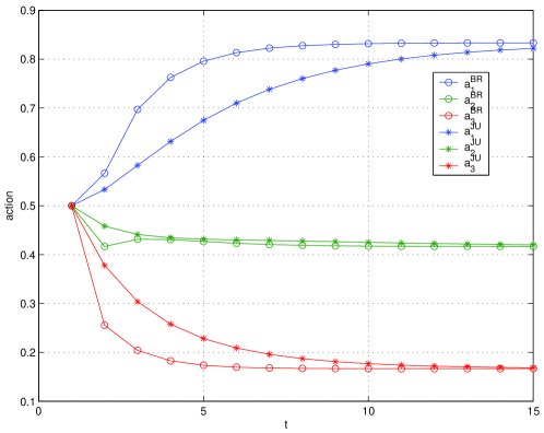
Figure 1: The trajectory of the best response and Jacobi update dynamics.

TABLE I: Actions and payoffs at NE and Pareto boundary.

	User 1	User 2	User 3
$a_{i}^{NE}$	$1.25$	$0.625$	$0.25$
$u_{i}^{NE}$	$3.4939$	$1.5625$	$1.25$
$a_{i}^{PB}$	$0.833$	$0.417$	$0.167$
$u_{i}^{PB}$	$3.8036$	$2.0833$	$2.0412$

TABLE II: Comparison between Type I and Type II games.

Games	Best response dynamics	Stability vs. efficiency	Fairness vs. parameter selection
Type I	local stability $\Leftarrow$ global convergence	stable at near-Pareto-optimal points	$u_{n}\varpropto\tau_{n}/\lambda_{n}$
Type II	local stability $\Leftrightarrow$ global convergence	stable at the Pareto boundary	$\omega_{n}=\tau_{n}/\lambda_{n}$ at the Pareto boundary

References

• [1] E. Altman, T. Boulogne, R. El-Azouzi, T. Jimenez, and L. Wynter, “A survey on networking games in telecommunications,” Computer Operation Research, vol. 33, pp. 286-311, Feb. 2006.
• [2] A. MacKenzie and S. Wicker, “Game Theory and the Design of Self-Configuring, Adaptive Wireless Networks,” IEEE Commun. Magazine, vol. 39, pp. 126-131, Nov. 2001.
• [3] V. Srivastava, J. Neel, A. MacKenzie, R. Menon, L.A. DaSilva, J. Hicks, J.H. Reed, and R. Gilles, “Using game theory to analyze wireless ad hoc networks,” IEEE Commun. Surveys Tutorials, vol. 7, pp. 46-56, 4th Quart. 2005.
• [4] M. Felegyhazi and J. P. Hubaux, “Game Theory in Wireless Networks: A Tutorial”, in EPFL technical report, LCA-REPORT-2006-002, February, 2006.
• [5] R. W. Lucky, “Tragedy of the commons,” IEEE Spectrum, vol. 43, no. 1, p. 88, Jan 2006.
• [6] D. Yao, “S-modular games with queueing applications,” Queueing Syst., vol. 21, pp. 449-475, 1995.
• [7] E. Altman and Z. Altman, “S-modular games and power control in wireless networks”, IEEE Trans. Automatic Control, vol. 48, no. 5, pp. 839-842, May, 2003.
• [8] R. Rosenthal, “A class of games possessing pure-strategy Nash equilibria”, International Journal of Game Theory, vol. 2, pp. 65-67, 1973.
• [9] G. Scutari, S. Barbarossa, D. P. Palomar, “Potential games: A framework for vector power control problems with coupled constraints,” Proc. IEEE ICASSP, Toulouse, May 2006.
• [10] R. Johari and J. N. Tsitsiklis, “Efficiency loss in a network resource allocation game,” Mathematics of Operations Research, vol. 29, no. 3, pp. 407-435, 2004.
• [11] T. Roughgarden and E. Tardos, “How Bad is Selfish Routing?”, Journal of the ACM, vol. 49, no. 2, pp. 236-259, Mar. 2002.
• [12] M. Chiang, S. H. Low, A. R. Calderbank, and J. C. Doyle, “Layering as optimization decomposition,” Proceedings of the IEEE, vol. 95, pp. 255-312. Jan 2007.
• [13] W. Saad, Z. Han, M. Debbah, A. Hjøungnes, and T. Başar, “Coalitional Game Theory for Communication Networks: A Tutorial,” IEEE Signal Processing Magazine, to appear.
• [14] Y. Su and M. van der Schaar, “Conjectural Equilibrium in Multi-user Power Control Games”, IEEE Trans. Signal Process., to appear.
• [15] Y. Su and M. van der Schaar, “Dynamic Conjectures in Random Access Networks Using Bio-inspired Learning”, UCLA Technical Report, Mar. 2009.
• [16] Z. Zhang and C. Douligeris, “Convergence of synchronous and asynchronous greedy algorithm in a multiclass telecommunications environment,” IEEE Tran. Commun., vol. 40, pp. 1277-1281, 1992.
• [17] P. Dubey, “Inefficiency of Nash equilibria,” Mathematics of Operations Research, pp. 1-8, 1986.
• [18] R. Myerson, Game Theory, Harvard University Press, 1991.
• [19] S. Boyd and L. Vandenberghe, Convex Optimization, Cambridge University Press, 2004.
• [20] M. P. Wellman and J. Hu, “Conjectural equilibrium in multiagent learning,” Machine Learning, vol. 33, pp. 179-200, 1998.
• [21] C. Figuières, A. Jean-Marie, N. Quérou, and M. Tidball, Theory of Conjectural Variations, World Scientific Publishing, 2004.
• [22] C. Douligeris and R. Mazumdar, “A game theoretic perspective to flow control in telecommunication networks,” J. Franklin Inst., vol. 329, no. 2, pp. 383-402, 1992.
• [23] R. La and V. Anantharam, “Utility based rate control in the internet for elastic traffic,” IEEE/ACM Trans. Networking, vol. 10, no. 2, pp. 271-286, Apr 2002.
• [24] M. R. Spiegel, Mathematical Handbook of Formulas and Tables. New York: McGraw-Hill, 1968.
• [25] A. Granas and J. Dugundji, Fixed Point Theory, New York: Springer-Verlag, 2003.
• [26] F. P. Kelly, “Charging and rate control for elastic traffic,” European Transactions on Telecommunications, vol. 8, pp. 33-37, 1997.
Refer to caption