Two Exoplanets Discovered at Keck Observatory

Abstract

We present two exoplanets detected at Keck Observatory. HD 179079 is a G5 subgiant that hosts a hot Neptune planet with $\mbox{$M\sin i$}=27.5$ $M_{\oplus}$ in a 14.48 d, low-eccentricity orbit. The stellar reflex velocity induced by this planet has a semiamplitude of $K=6.6$ m s^-1. HD 73534 is a G5 subgiant with a Jupiter-like planet of $\mbox{$M\sin i$}=1.1$ $M_{\rm Jup}$ and $K=16$ m s^-1 in a nearly circular 4.85 yr orbit. Both stars are chromospherically inactive and metal-rich. We discuss a known, classical bias in measuring eccentricities for orbits with velocity semiamplitudes, $K$, comparable to the radial velocity uncertainties. For exoplanets with periods longer than 10 days, the observed exoplanet eccentricity distribution is nearly flat for large amplitude systems ($K>80$ m s^-1), but rises linearly toward low eccentricity for lower amplitude systems ($K>20$ m s^-1).

1 Introduction

Since the discovery of 51 Peg (Mayor & Queloz, 1995), more than 300 exoplanets have been detected, mostly by Doppler measurements of stellar reflex velocities. The distributions of these exoplanet masses, semi-major axes, and orbital eccentricities provide evidence for planet formation and orbital evolution (Marcy et al., 2008). Currently, known exoplanets have a median mass of about 1 $M_{\rm Jup}$ and median semi-major axis of about 1 AU. Early exoplanet discoveries were mostly massive gas giants in short-period orbits because such orbits have velocity amplitudes much larger than measurement errors and because it takes less time to observe many orbits and get complete phase coverage. Steady improvements in Doppler precision have enabled the recent detection of planets with $\mbox{$M\sin i$}\sim 10\mbox{$M_{\oplus}$}$ (Howard et al., 2009; Rivera et al., 2005; Udry et al., 2007; Mayor et al., 2009), despite velocity semiamplitudes of only a few m s^-1.

Here, we present two new exoplanets detected at Keck Observatory as part of a search for hot Neptune-mass and other low-amplitude planets. The host stars were originally observed as part of the N2K program, a survey of metal-rich stars to detect hot Jupiters (Fischer et al., 2005). We continued observing a subset of promising N2K stars to search for exoplanets with lower velocity amplitudes, including Neptune mass planets in short period orbits (“hot Neptunes”). The hot Neptune sample consists of about a hundred N2K stars with low chromospheric activity, low $v\sin i$, and a velocity scatter greater than $2\sigma$ but less than 20 m s^-1. The hot Neptune sample inherits from the N2K survey a selection bias in favor of high-metallicity stars that increases the probability of detecting massive planets (Fischer & Valenti, 2005) and a Malmquist bias that increases the number of subgiants because stellar magnitude was a factor in target selection.

The orbital eccentricity distribution is an interesting characteristic of detected exoplanets. In sharp contrast to planets in our solar system, exoplanets with orbital periods longer than 10 d have eccentricities that range from circular to greater than 0.9, with a median eccentricity of 0.24. Planets with orbital periods shorter than about 10 d are expected to circularize over time via tidal interactions with the host star. Consistent with this prediction, the median eccentricity of exoplanets with orbital periods shorter than 10 days is only 0.013. Interesting exceptions include HD 185269b (Johnson et al., 2006, $P=6.84$ d, $e=0.30$), HD 147506b (Bakos et al., 2007, $P=5.6$ d, $e=0.5$), and (Johns-Krull et al., 2008, $P=3.2$ d, $e=0.26$). Precise eccentricity measurements for planets with a range of periods, masses, and ages help to empirically constrain orbital evolution models.

2 Data and Methods

2.1 Spectroscopic Observations

We used the HIRES spectrometer (Vogt et al., 1994) at Keck Observatory for 3–5 years to obtain a temporal sequence of $R=65,000$ spectra for each star. An iodine cell in the beam imprinted a rich set of molecular absorption lines on the stellar spectrum. These iodine lines constrain the wavelength scale, point-spread functions, and Doppler shift for each individual observation (Marcy & Butler, 1992; Butler et al., 1996). An exposure meter was used to adjust each exposure time to achieve a consistent signal-to-noise ratio of 200 per extracted pixel, which alleviates some types of systematic errors. The exposure meter was also used to determine the photon-weighted midpoint of each exposure, which improves the precision of the barycentric velocity correction.

Spectra obtained after 2004 August with the new HIRES detector mosaic include the Ca II H & K lines, which provide a diagnostic of chromospheric activity. We characterized line core emission in terms of the S index (Vaughan et al., 1978; Duncan et al., 1991). To improve measurement precision, we matched the line wings and neighboring continua for each observation of a given star to the mean value for all observations of that star (Isaacson, 2009).

2.2 Photometric Observations

We obtained photometric observations of HD 179079 and HD 73534 with the T12 0.8 m automated photometric telescope (APT) at Fairborn Observatory in southern Arizona. The T12 APT and its precision photometer are very similar to the T8 APT described in Henry (1999). The precision photometer uses two temperature-stabilized EMI 9124QB photomultiplier tubes to measure photon count rates simultaneously through Strömgren $b$ and $y$ filters.

The telescope was programmed to measure each target star with respect to three nearby comparison stars in the following sequence: DARK, A, B, C, D, A, SKY_A, B, SKY_B, C, SKY_C, D, SKY_D, A, B, C, D, where A, B, and C are comparison stars and D is the program star. Each complete sequence, referred to as a group observation, was reduced to form three independent measures of each of the six differential magnitudes D$-$A, D$-$B, D$-$C, C$-$A, C$-$B, and B$-$A. The differential magnitudes were corrected for differential extinction with nightly extinction coefficients and transformed to the standard Strömgren system with yearly mean transformation coefficients. To filter out observations taken under non-photometric conditions, an entire group of observation was discarded if the standard deviation of any of the six mean differential magnitudes exceeded 0.01 mag. We also combined the Strömgren $b$ and $y$ differential magnitudes into a single $(b+y)/2$ passband to improve the precision.

2.3 Stellar Analysis

We determined stellar properties by analyzing one spectrum of each star obtained without the iodine cell. We used SME (Valenti & Piskunov, 1996) and the procedure of Valenti & Fischer (2005) to fit each observed spectrum with a synthetic spectrum, obtaining the stellar effective temperature $T_{\rm eff}$, surface gravity ${\rm\log g}$, metallicity [M/H], projected rotational velocity $v\sin i$, and elemental abundances of Na, Si, Ti, Fe, and Ni. Our [M/H] parameter here (as in Valenti & Fischer, 2005) scales solar abundances for elements other than Na, Si, Ti, Fe, and Ni that have significant spectral lines in our fitted wavelength intervals. We report iron abundance [Fe/H] rather than [M/H] because [Fe/H] is better defined. We use the abundance of Si relative to iron [Si/Fe] as a proxy for alpha-element enrichment [$\alpha$/Fe].

We obtained a bolometric correction (BC) for each star by interpolating the “high-temperature” grid of VandenBerg & Clem (2003) to our spectroscopically determined $T_{\rm eff}$, ${\rm\log g}$, and [Fe/H]. Using formulae and constants in Valenti & Fischer (2005), we calculated stellar luminosity from apparent visual magnitude $V$, BC, and distance $d$ of the star, and then stellar radius $R_{\star}$ from $L_{\star}$ and $T_{\rm eff}$.

Following Valenti & Fischer (2005), we determined stellar mass $M_{\star}$, age, and surface gravity $\log g_{\rm iso}$ by interpolating tabulated Yonsei–Yale isochrones (Demarque et al., 2004), first to our measured [$\alpha$/Fe], then to our measured [Fe/H], then to our measured $T_{\rm eff}$, and finally to the observed $L_{\star}$. This yields zero, one, or multiple possible stellar models. We repeat the interpolation for a grid of $17^{4}$ values of [$\alpha$/Fe], [Fe/H], $T_{\rm eff}$, and $L_{\star}$ that span the range of measurement uncertainties. We weight each outcome by the likelihood of the interpolation parameter and by the lifetime of the output evolutionary state. This favors relatively stable main-sequence states over rapidly evolving states.

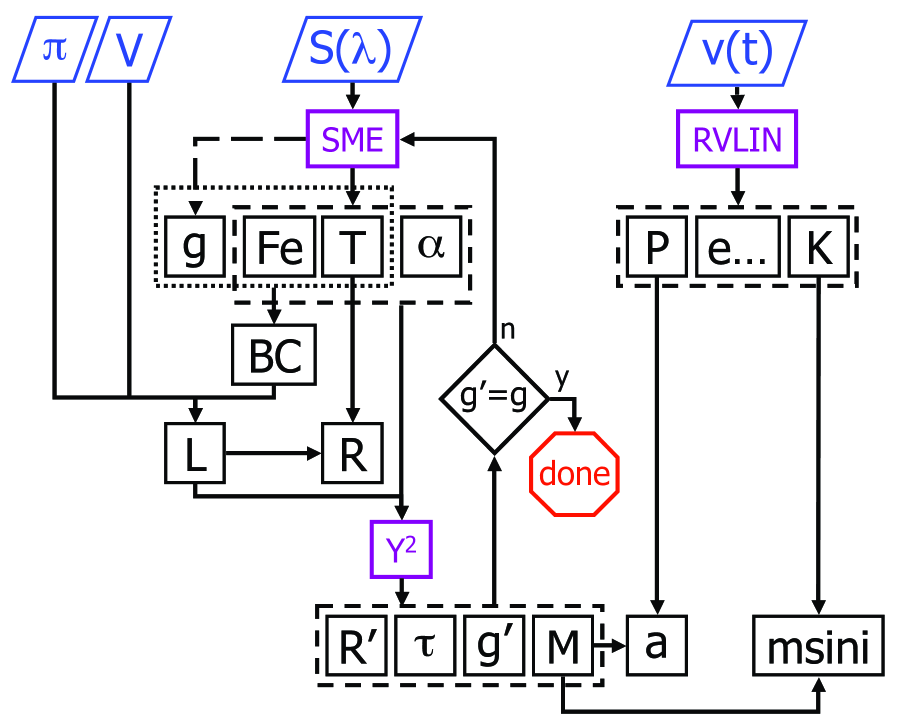
Figure 1: Graphical representation of the analysis flow. Observables in the top row are parallax, apparent visual magnitude, a high-resolution spectrum, and measured radial velocities. The left side shows the spectroscopic (SME) and isochrone (Y²) analysis, while the right side shows the orbital analysis (RVLIN). Symbols for derived quantities are as described in the text, but with Fe for [Fe/H], $\alpha$ for [$\alpha$/Fe], $\tau$ for age, and $g^{\prime}$ for $g_{\rm iso}$. The arrow pointing up to the $g^{\prime}=g_{\rm iso}$ decision diamond illustrates a new outer loop that enforces consistency between spectroscopic and isochrone gravities. (A color version of this figure is available in the online journal.)

The Valenti & Fischer (2005) procedure described above does not require agreement between ${\rm\log g}$ from spectroscopy and $\log g_{\rm iso}$ from isochrones, though the two are usually close. Here we introduce an outer iteration loop in which the SME analysis is repeated with ${\rm\log g}$ fixed at the value of $\log g_{\rm iso}$ from the preceding iteration. After a few iterations, the output ${\rm\log g}$ from SME agrees with the input $\log g_{\rm iso}$. The price for this self-consistency is a greater dependence on models and worse $\chi_{\nu}^{2}$ for the spectrum fits. However, we are already completely dependent on stellar evolution models for $M_{\star}$, and systematic errors in spectral line data dominate $\chi_{\nu}^{2}$. Using evolutionary tracks as an additional constraint on ${\rm\log g}$ while fitting spectra should improve the accuracy of the other derived parameters. We give examples later in this paper. Figure 1 shows the analysis procedure graphically.

2.4 Orbital Analysis

Using the periodogram procedure described in Marcy et al. (2005), we analyzed the velocity time series for each star to identify planet candidates and prospective periods. Once a sufficient number of observations were obtained, we fitted the velocities with Keplerian orbits, using a Levenberg-Marquardt algorithm (Wright & Howard, 2009). The free parameters are orbital period $P$, velocity semiamplitude $K$, eccentricity $e$, time of periastron passage $T_{p}$, argument of periastron referenced to the line of nodes $\omega$, and velocity offset of the center-of-mass $\gamma$.

When fitting Keplerian models, we adopted a total variance equal to the quadrature sum of our velocity measurement precision (1–2 m s^-1) and a velocity jitter term of 3.5 m s^-1. Jitter includes both systematic measurement errors and astrophysical velocity perturbations caused by photospheric flows and inhomogeneities. Our adopted jitter of 3.5 m s^-1 for the two subgiants in this paper yields $\chi_{\nu}^{2}$ near unity and is consistent with the range of values in Wright (2005). The exact choice of jitter has an insignificant effect on our derived values of $P$ and $K$.

We used $10^{5}$ Monte Carlo trials to estimate uncertainties in our derived orbital parameters. In each trial, we constructed a simulated observation by adding errors to the Keplerian model that best matches our observed velocities. These errors were selected randomly from the distribution of observed residuals. A particular residual could be used multiple times or not at all in any given trial. We fitted each simulated observation using exactly the same procedure that we used to analyze the actual observation. Each trial included a periodogram analysis, which for stars with few observations can occasionally yield a distinct period. After $10^{5}$ trials, the width of the distribution function for a particular orbital parameter yields an estimate of the uncertainty in our observed value of that parameter.

3 HD 179079

3.1 Stellar Characteristics

HD 179079 (HIP 94256, $V=7.95$, $B-V=0.744\pm 0.013$) is a G5 subgiant at a distance of $65.5\pm 3.3$ pc (Perryman & ESA, 1997; van Leeuwen, 2008). High-resolution spectroscopic analysis (see Section 2.3) yields $\mbox{$T_{\rm eff}$}=5684\pm 44$ K, $\mbox{${\rm\log g}$}=4.06\pm 0.06$, $\mbox{\rm[Fe/H]}=+0.25\pm 0.03$ dex, and $\mbox{$v\sin i$}<1.0$ km s^-1. These spectroscopic results imply a bolometric correction of $\mbox{BC}=-0.094$ and hence a stellar luminosity of $\mbox{$L_{\star}$}=2.41\pm 0.27$ $L_{\odot}$, where the uncertainty in luminosity is dominated by the uncertainty in distance. Using $L_{\star}$ and $T_{\rm eff}$, we obtain a stellar radius of $\mbox{$R_{\star}$}=1.60\pm 0.09$ $R_{\odot}$. Stellar evolutionary tracks imply a stellar mass of $\mbox{$M_{\star}$}=1.15\pm 0.03$ $M_{\odot}$.

HD 179079 is chromospherically inactive, based on weak emission in the cores of the Ca II H & K lines. We measure $S_{\rm HK}$= 0.153, which yields $\mbox{$\log R^{\prime}_{\rm HK}$}=-5.06$ and implies a rotation period of roughly 38 d (Noyes et al., 1984). The level of chromospheric activity implies an approximate age of 7 Gyr, which is consistent with the 68% credible interval of 6.1–7.5 Gyr from the isochrone analysis. We estimate that surface motion in the photosphere of this early subgiant contributes 3.5 m s^-1 of velocity jitter that we add in quadrature to velocity measurement uncertainties, when modeling the data. Table 1 summarizes the stellar parameters. Table 2 shows how key stellar parameters changed during the iteration procedure introduced in Section 2.3.

3.2 Doppler Observations and Keplerian Fit

We obtained 74 observations of HD 179079 beginning in 2004 July. The observation dates, radial velocities and measurement uncertainties are listed in Table 3. Typical exposure times were about 2 minutes. The median velocity measurement uncertainty is 1.2 m s^-1, which is small compared to the velocity jitter of 3.5 m s^-1.

Figure 2 shows a periodogram of the 74 measured radial velocities, with an unambiguous peak in power at 14.46 days. The false alarm probability (FAP) is less than 0.0001, i.e., the probability that a random set of data would produce a peak with the observed power is less than 0.01%. The FAP test checks for spurious peaks that can arise because of window functions in the data. To calculate the FAP, simulated velocities for actual observation times were drawn randomly from the distribution of observed velocities, allowing reuse of any value. After $10^{4}$ trials, we found no peaks for simulated data with as much power as the observed peak at 14.48 days. Thus, the FAP is less than the reciprocal of the number of trials, i.e. less than $10^{-4}$.

Our best-fitting Keplerian model has a period $P=14.476\pm 0.011$ d, velocity semiamplitude $K=6.64\pm 0.60$ m s^-1, and eccentricity $e=0.12\pm 0.09$. Uncertainties for the orbital parameters were derived from Monte Carlo trials, as described in Section 2.4. The rms residual about the model fit is 3.9 m s^-1. Including jitter of 3.5 m s^-1, we find $\mbox{$\chi_{\nu}^{2}$}=1.04$. The eccentricity is poorly constrained, as indicated by the large uncertainty found in our Monte Carlo trials. A circular orbit yields $\mbox{$\chi_{\nu}^{2}$}=1.03$, which is as probable as the solution obtained with eccentricity and $T_{p}$ as free parameters. The challenge of measuring low eccentricities in low amplitude systems is discussed in Section 5.1.

Figure 3 shows the phase-folded RV data together with the Keplerian (solid line) and circular (dotted line) models that best fit the data. Observations are plotted using phases based on the Keplerian fit, rather than the circular fit. In this and subsequent velocity plots, error bars are dominated by velocity jitter, rather than velocity measurement precision. Adopting a stellar mass of $1.146\pm 0.028$ $M_{\odot}$, we derive a minimum mass of $\mbox{$M\sin i$}=27.5\pm 2.5$ $M_{\oplus}$ and a semi-major axis of $0.121\pm 0.001$ AU. The complete Keplerian orbital solution is given in Table 4.

3.3 Transit Search

Because the orbital period for this planet is relatively short, we have carried out an extensive search for transits, both with photometry (described in the following section) and by phase-folding the radial velocities to search for velocities that might have been obtained serendipitously during the $\sim 3$ hr transit window. As the planet traverses the stellar disk, it blocks light from first one side (say the approaching, blueshifted edge of the stellar disk) and then the other side (the receding, redshifted edge) of the star. Our Doppler analysis interprets the spectral line asymmetry as excess velocity shifts during ingress and egress. This phenomenon is known as the Rossiter-McLaughlin effect.

The amplitude of the Rossiter-McLaughlin effect increases with both projected stellar rotation velocity and planet size relative to the star. HD 179079 has a low rotational velocity ($\mbox{$v\sin i$}=0.5$ km s^-1) and a small radius (expected to be similar to Neptune for an $\mbox{$M\sin i$}=25.4$ $M_{\rm Jup}$ planet). Therefore, the amplitude of the Rossiter-McLaughlin effect is expected to be no more than our measurement errors of about 2 m s^-1 for HD 179079. Nevertheless, we phase-folded the radial velocities and calculated the ingress and egress times for eccentricities ranging from 0 to 0.1. Uncertainties in the orbital eccentricity lead to shifts of up to 16 hr in the prospective transit time at the epochs of our radial velocity measurements. Velocity residuals during these broad transits windows were no larger than velocity residuals at other orbital phases.

3.4 Photometry

Our 243 good brightness measurements of HD 179079 were made between 2007 June and 2008 June and cover parts of the 2007 and 2008 observing seasons. The comparison stars A, B, and C were HD 177552 ($V=6.51$, $B-V=0.36$, F1 V), HD 181420 ($V=6.57$, $B-V=0.44$, F2), and HD 180086 ($V=6.63$, $B-V=0.35$, F0), respectively. The differential magnitudes C$-$A, C$-$B, and B$-$A demonstrated that all three comparison stars were constant to 0.002 mag or better. To minimize the effect of any low-level intrinsic variation in the three comparison stars, we averaged the three D$-$A, D$-$B, and D$-$C differential magnitudes of HD 179079 within each group into a single value, representing the difference in brightness between HD 179079 and the mean brightness of the three comparison stars: $D-(A+B+C)/3$. The standard deviation of these ensemble differential magnitudes for the complete data set is 0.00190 mag. This is comparable to the typical precision of a single observation with this telescope, indicating there is little or no photometric variability in HD 179079.

Solar-type stars often exhibit brightness variations caused by cool, dark photospheric spots as they are carried into and out of view by stellar rotation (e.g., Gaidos, Henry, & Henry, 2000). Periodogram analyses of the D$-$A, D$-$B, and D$-$C differential magnitudes for HD 179079 yield no significant periodicity between 1 and 100 days, consistent with the star’s low level of chromospheric activity and its low $v\sin i$ (Table 1). We see no significant power at any period within a factor of 2 of 38 d, which is the rough rotation period implied by the chromospheric activity level.

The 243 ensemble $(b+y)/2$ differential magnitudes of HD 179079 are plotted in the top panel of Figure 4. Phases are computed from the orbital period given in Table 4 and the epoch JD $2,454,678.8\pm 0.67$, a recent time of mid-transit derived from the orbital elements. A least-squares sine fit on the orbital period yields a semiamplitude of only 0.00007 $\pm$ 0.00016 mag. This very low limit to photometric variability on the radial velocity period is strong evidence that the low-amplitude radial velocity variations observed in the star are, in fact, due to reflex motion induced by a low-mass companion and not to activity-induced intrinsic variations in the star itself (e.g., Paulson et al., 2004).

The photometric observations of HD 179079 near the predicted time of transit are replotted with an expanded horizontal scale in the bottom panel of Figure 4. The solid curve shows the predicted time (0.00 phase units) and duration ($\pm 0.009$ phase units) of transits with a depth of 0.08% computed from estimated stellar and planetary radii. The error bar in the upper right of both panels represents the mean precision of a single observation (0.0019 mag). The horizontal error bar immediately below the transit in both panels represents the uncertainty in the predicted time of mid-transit ($\pm 0.67$ days or $\pm 0.046$ phase units). It is clear from the data in the bottom panel that we cannot rule out the possibility of shallow transits of HD 179079b.

4 HD 73534

4.1 Stellar Characteristics

HD 73534 (HIP 42446, $V=8.23$, $B-V=0.962\pm 0.021$) is a G5 subgiant at a distance of $81.0\pm 4.9$ pc (ESA, 1997; van Leeuwen, 2008). High-resolution spectrum synthesis modeling yields $\mbox{$T_{\rm eff}$}=5041\pm 44$ K, $\mbox{${\rm\log g}$}=3.78\pm 0.06$, $\mbox{\rm[Fe/H]}=+0.23\pm 0.03$ dex, and $\mbox{$v\sin i$}<1.0$ km s^-1. The resulting bolometric correction of $\mbox{BC}=-0.266$ yields a stellar luminosity of $\mbox{$L_{\star}$}=3.33\pm 0.43$ $L_{\odot}$. Combining $T_{\rm eff}$ and $L_{\star}$, we obtain a stellar radius of $\mbox{$R_{\star}$}=2.39\pm 0.16$ $R_{\odot}$. Stellar evolutionary tracks yield a stellar mass of $\mbox{$M_{\odot}$}=1.23\pm 0.06$ $M_{\odot}$.

HD 73534 has minimal emission in the Ca II H & K line cores, implying chromospheric inactivity, which is typical for subgiants (Wright, 2004). Applying Noyes et al. (1984) relationships that were calibrated using main-sequence stars, our measured $\mbox{$S_{\rm HK}$}=0.155$ yields $\mbox{$\log R^{\prime}_{\rm HK}$}=-5.13$ and a crude rotation period of 53 d. The level of chromospheric activity implies an approximate age of 9 Gyr, which differs significantly from the 68% credible interval of 5.2–7.2 Gyr from the isochrone analysis.

Subgiants have slightly more velocity jitter than inactive main-sequence stars, as evidenced by the greater rms scatter seen in subgiants without detected planets. We estimate that the intrinsic stellar jitter of HD 73534 is 3.5 m s^-1. Table 1 lists our derived stellar parameters. Table 6 shows how key parameters for HD 73435 changed during the iteration procedure introduced in Section 2.3.

4.2 Doppler Observations and Keplerian Fit

We began observing HD 73534 in 2004 July as part of the N2K program (Fischer et al., 2005). No short-period velocity variations were detected, but we continued to obtain a few velocity measurements each year to map out an emerging low-amplitude, long-period planet. We now have a total of 30 observations that span five years. The raw velocity measurements have a precision of 1.1 m s^-1, but the (unmodeled) rms is 13.8 m s^-1. Exposure times were two to five minutes. The observation dates, radial velocities and associated uncertainties are listed in Table 5.

The best fit Keplerian model has a period, $P=1770\pm 40$ d, velocity semiamplitude, and $K=16.2\pm 1.1$ m s^-1. The orbital eccentricity, $e=0.07\pm 0.07$, is not significantly different from zero. The rms residual of the fit is 3.36 m s^-1 with $\chi_{\nu}^{2}$= 0.91 after including stellar jitter of 3.5 m s^-1. Adopting a stellar mass of $\mbox{$M_{\odot}$}=1.228\pm 0.060$ $M_{\odot}$, we derive $\mbox{$M\sin i$}=1.103\pm 0.087$ $M_{\rm Jup}$ and a semimajor axis of $a=3.067\pm 0.068$ AU. The complete set of orbital parameters are listed in Table 4. Figure 5 shows the phased radial velocity data with the best-fit Keplerian (solid line) and circular (dotted line) models overplotted.

4.3 Photometry

From 2004 November to 2008 December, we collected 521 good photometric observations of HD 73534 during five consecutive observing seasons. We do not see a correlation between radial velocities and activity or photometric measurements, however, we present the photometric data for posterity.

The comparison stars A, B, and C were HD 72943 ($V=6.33$, $B-V=0.34$, F0 IV), HD 73347 ($V=8.00$, $B-V=0.40$, F0), and HD 73821 ($V=7.82$, $B-V=0.30$, F0), respectively. Comparison star A (HD 72943) was found to be variable with an amplitude of 0.010 mag and a period of 0.0919 d; it is probably a $\delta$ Scuti variable. Comparison stars B and C were constant to 0.002 mag or better, so we created and analyzed ensemble differential magnitudes using only those two comparison stars: $D-(B+C)/2$.

The standard deviation of all 521 observations is 0.0018 mag, which is the typical precision of our photometry. To search for low-amplitude periodic brightness variations, we calculated power spectra for each observing season and combined the results. We did not detect any significant power for periods between 1 and 100 days, which more than spans the range of plausible rotation periods. The absence of significant optical variability on rotational time scales is consistent with the low level of chromospheric activity detected in HD 73534.

To search for low-amplitude, brightness variations on longer time scales, we computed the mean brightness for each of our five observing seasons. For HD 73534, the seasonal means have a full range of 0.0029 mag and a standard deviation of 0.0012 mag. For the two comparison stars, the seasonal mean values of $C-B$ have a full range of only 0.0014 mag and a standard deviation of only 0.0006 mag, a factor of 2 smaller. Wright et al. (2008) demonstrated that for solar-type stars, we can measure seasonal means with a precision (standard deviation) of 0.0002 mag. HD 73534 varies by about 0.001 mag from year to year, but the variations are not systematic.

Finally, we compared our seasonal mean brightness measurements with our seasonal mean radial velocities, obtaining a linear correlation coefficient of 0.3345. With only five data points, the correlation coefficient would be at least this large 42% of the time, if brightness and velocity are uncorrelated random variables. A significant correlation between stellar brightness and radial velocity would raise doubts about the planetary origin of the stellar velocity variations, but in this case we do not detect a significant correlation.

5 Eccentricity

5.1 Eccentricity Measurement Bias

Eccentricity cannot be negative. For a circular orbit, errors in individual radial velocity measurements can only drive the measured eccentricity away from the true value of zero (e.g., Shen & Turner, 2008). As radial velocity planet searches push to lower amplitude systems, this bias becomes significant for low eccentricity planets.

When observed velocity constraints for a circular orbit are uniformly distributed in orbital phase (approximately true for most radial velocity planet detections), Lucy (1971) derives the probability distribution for measured eccentricity,

$$p(e)de={e\over\sigma_{e}^{2}}\exp\left(-{e^{2}\over 2\sigma_{e}^{2}}\right)de,$$ (1)

where the eccentricity uncertainty, $\sigma_{e}$, is given by Luyten (1936) as

$$\sigma_{e}={\sigma\over K}\left({2\over N}\right)^{0.5},$$ (2)

where $\sigma$ is the typical uncertainty in velocity and $N$ is the number of velocity measurements. The detection of nonzero eccentricity with better than 95% confidence requires approximately $e/\sigma_{e}>2.45$.

To demonstrate the challenge in recovering zero eccentricity for HD 179079, we created $10^{5}$ synthetic data sets based on an $e=0$ fit of the observed velocities for HD 179079. We added errors by drawing randomly (with replacement) from the observed distribution of residuals about the $e=0$ fit. Finally, we fitted each simulated data set with a Keplerian, leaving eccentricity as a free parameter. Figure 6 shows the resulting distribution of imprecisely measured eccentricities.

Even though we simulated a circular orbit, the measured eccentricities in Figure 6 are significantly biased toward positive values. The eccentricity distribution has a median of 0.164 and a standard deviation of 0.075. Clearly, our observed eccentricity of $0.115\pm 0.087$ does not rule out a circular orbit.

Our $N=74$ observations of HD 179079 are spread nearly uniformly in orbital phase and have an rms residual of $\sigma=3.9$ m s^-1 (dominated by stellar jitter with an amplitude of about 3.5 m s^-1). With a measured eccentricity of $e=0.11$ and a velocity semiamplitude of $K=6.6$ m s^-1, we obtain $e/\sigma_{e}=1.1$, which is well below the approximate threshold for a significant detection.

The dotted line in Figure 6 shows the predicted distribution according to Equation 1, but with $\sigma=4.2$ m s^-1, rather than the observed rms of 3.9 m s^-1, to better match the observed distribution. This slight excess in $\sigma_{e}$ relative to Equation 2 may be due to velocity constraints that are not uniformly distributed in phase or non-optimal behavior of the Levenberg-Marquardt algorithm used to fit Keplerian orbits. The Keplerian fitting routine also returns the limiting value of $e=0$ more often than predicted by the analytic approximation.

5.2 Observed Eccentricity Distributions

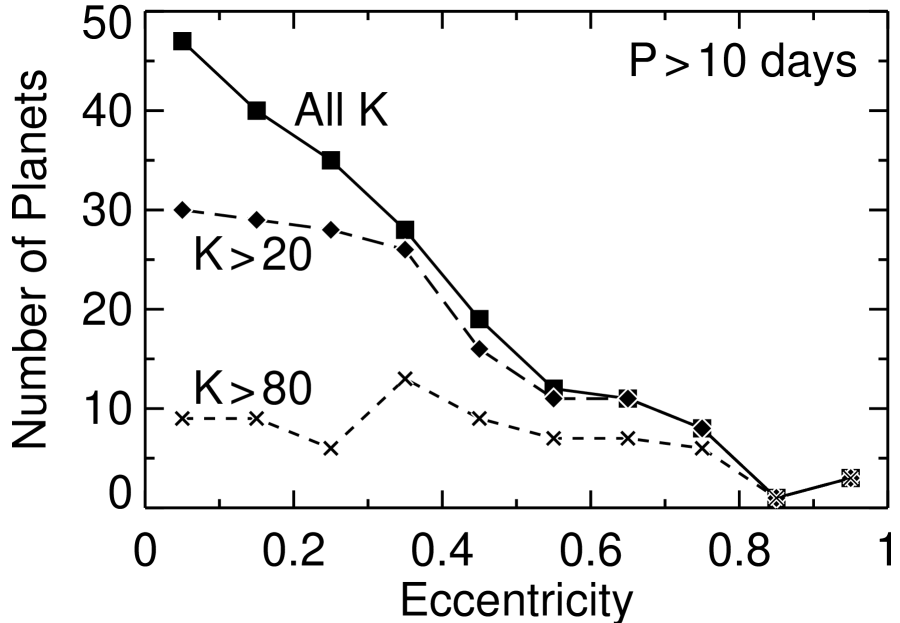
Figure 7: Ignoring planets with periods shorter than 10 days, which may have circularized, the eccentricity distribution for known planets decreases linearly from $e=0$ to $e=0.6$. For planets with $K>20$ m s^-1, the distribution is much flatter from $e=0$ to $e=0.4$ and then declines. For planets with $K>80$ m s^-1, the distribution is flat all the way up to $e=0.8$. These distributions may reflect an observational bias against detecting high eccentricity planets with velocity semiamplitudes $K$ near the detection limit, in which case the observed distribution for large $K$ may represent the intrinsic eccentricity distribution for giant planets.

Figure 7 shows observed eccentricity distributions for 204 well-characterized planets, a subset of 163 planets with $K>20$ m s^-1, and a further subset of 70 planets with $K>80$ m s^-1. In all three cases, we exclude 53 planets with periods less than 10 days that may have experienced orbital evolution due to tidal interaction with the star.

The observed eccentricity distributions become flatter as lower $K$ planets are excluded. This flattening cannot be due to eccentricity measurement bias (Section 5.1), which would create the opposite slope, as positively biased measurements for lower $K$ planets are included in the distribution. The sequence of observed eccentricity distributions in Figure 7 may reflect dynamical processes that link planet mass and eccentricity (e.g., Jurić & Tremaine, 2008; Ford & Rasio, 2008, for high mass planets), but below we discuss briefly a possible origin based on observational bias.

At fixed $K$, planets in more eccentric orbits induce large velocity shifts for a smaller fraction of the orbit, making them harder to detect. For this reason, the dependence of the observed eccentricity distribution on $K$ threshold may reflect an observational bias, rather than measurement bias. If true, the flat eccentricity distribution for $K>80$ m s^-1 in Figure 7 may be the true distribution for giant planets. For the $K>20$ m s^-1 threshold, detection of highly eccentric planets may become more difficult, causing the eccentricity distribution to drop above $e=0.4$. Finally, the lowest $K$ planets may be very difficult to detect reliably except in nearly circular orbits. If this hypothesis is true, a large population of low $K$, high $e$ planets have yet to be detected. It would be interesting to quantify the expected detection bias as a function of eccentricity in actual radial velocity planet search programs.

6 Discussion

We have presented two exoplanets detected at Keck Observatory in a search for hot Neptunes and other low-amplitude planets. The two planets have masses $1.61\pm 0.15$ and $20.7\pm 2.2$ times the mass of Neptune. The radial velocity semiamplitudes of these planets are $6.64\pm 0.60$ and $16.3\pm 1.3$ m s^-1, respectively. Both host stars are metal rich subgiants, which is consistent with the selection criteria of the parent N2K sample (Fischer et al., 2005).

HD 179079 is a G5 subgiant with an $\mbox{$M\sin i$}=27.5\pm 2.5$ $M_{\oplus}$ planet in a low eccentricity, 14.48 d orbit. The semivelocity amplitude of the star is only 6.6 m s^-1, making this a challenging detection. Although the periodogram signal was apparent after about 30 observations, we obtained 74 Doppler measurements before announcing this planet because of the small velocity amplitude and concern about jitter in this slightly evolved star. However, the periodogram power continues to grow at the same period and the rotational period for this subgiant is expected to be about 38 days.

HD 73534b is a $\mbox{$M\sin i$}=1.103\pm 0.087$ $M_{\rm Jup}$ planet in a nearly circular 4.85 yr orbit around a metal-rich subgiant. This is one of the handful of known planets (e.g., Wright et al., 2008) in low low eccentricity orbits that did not migrate well inside the ice line in the parent protoplanetary disk. As precise Doppler observations extend over longer time baselines, more such planets will be discovered.

Numerical simulations of the efficiency of orbital migration (Ida & Lin, 2004, 2008, Figure 5) provide predictions for the mass and semi-major axis distribution of exoplanets. The distribution of gas giant planets provides a good match to the numerical prescriptions, however the most remarkable feature of the simulations is the prediction of a planet “desert.” Over a wide range of initial conditions (migration speeds, stellar metallicity, and mass or surface density in the protoplanetary disks), these results consistently show a paucity of intermediate mass ($M_{p}\sim 10-100$ $M_{\oplus}$) planets closer than a few AU. One of the two planets presented here, HD 179079, populates this “no planet” region, providing an interesting, benchmark for future simulations.

The detected stellar velocity amplitudes are small for both new planets. Figure 8 compares the masses and orbital periods of these new planets with 256 known exoplanets. The Doppler technique has progressed both in precision and duration to a point where the detection of planets with amplitudes of 5 m s^-1 define a boundary for orbital periods out to 10 years. Clearly, we stand at the threshold for detecting the signpost of our solar system, Jupiter, with a 12 m s^-1 velocity amplitude in a 11.7 year orbit.

Figure 2: Periodogram of 74 radial velocity measurements for HD 179079. The prominent peak at 14.46 d is consistent with the $14.476\pm 11$ d period returned by a Keplerian fit of the measured velocities. The next four strongest peaks (labeled in the figure) are significantly weaker.

Figure 3: Phased radial velocities for HD 179079 reveal an orbital period of 14.48 d, a velocity amplitude of 6.64 m s^-1, and an eccentricity of 0.12. Error bars illustrate the quadrature sum of the velocity precision for each measurement and 3.5 m s^-1 of jitter (systematic errors and/or intrinsic stellar variability). The Keplerian model is overplotted with a solid line and the dotted line shows the model with eccentricity fixed to zero. Adopting a stellar mass of 1.15 $M_{\odot}$ we derive a planet mass, $\mbox{$M\sin i$}=28$ $M_{\oplus}$ and orbital radius of 0.122 AU.

Figure 4: Top panel: the 243 ensemble $D-(A+B+C)/3$ photometric observations of HD 179079 in the combined Strömgren $(b+y)/2$ passband, acquired with the T12 0.8 m APT over two observing seasons and plotted modulo the 14.476 d orbital period of the inner companion. Phase 0.0 corresponds to a predicted time of mid transit. A least-squares sine fit at the orbital period yields a semiamplitude of only $0.00007\pm 0.00016$ mag. Bottom panel: the photometric observations of HD 179079 near the predicted time of transit plotted with an expanded scale on the abscissa. The solid curve shows the predicted time of transit with a drop in stellar brightness of 0.08% ($\sim 0.00087$ mag). The error bar in the upper right of both panels represents the mean precision of a single observation (0.0019 mag). The error bar immediately below the predicted time of transit in both panels represents the uncertainty in the predicted time of mid-transit ($\pm 0.67$ days or $\pm 0.046$ phase units).

Figure 5: Radial velocities for HD 73534 are fit with an orbital period of 1770 d, velocity amplitude of 16.2 m s^-1, and a nearly circular orbit. Error bars illustrate the quadrature sum of the velocity precision for each measurement and 3.5 m s^-1 of jitter (systematic errors and/or intrinsic stellar variability). The assumed stellar mass of 1.23 $M_{\odot}$ yields $\mbox{$M\sin i$}=1.10$ $M_{\rm Jup}$ and a semi-major axis of 3.07 AU.

Figure 6: Probability that we would measure an eccentricity $e$ for our 74 Keck observations of HD 179079, if the true eccentricity is zero, $e_{*}=0$. The asymmetric distribution of measured eccentricities has a median of 0.123 and a standard deviation of 0.075, despite a true eccentricity of zero. The hatched regions show 34.1% of the distribution on either side of the median.

Figure 8: Velocity semiamplitude vs. orbital period for planets with radial velocity detections. The two planets announced in this paper are indicated by filled squares. Diagonal dashed lines show the approximate locus of Jupiter and Neptune mass planets, assuming $M=\mbox{$M_{\odot}$}$, $e=1$, and $\sin i=1$. Detecting low mass planets with long periods is particularly challenging.

Table 1: Stellar Parameters

Parameter	HD 179079	HD 73534
Spectral type	G5 IV	G5 IV
Distance (pc)	65.5(3.3)	81.0(4.9)
$V$	7.95	8.23
$B-V$	0.744(13)	0.962(21)
$T_{\rm eff}$ (K)	5684(44)	5041(44)
${\rm\log g}$	4.062(60)	3.780(60)
[Fe/H]	0.250(30)	0.232(30)
$v\sin i$ (km s-1)	$<1.0$	$<1.0$
BC	$-$0.094	$-$0.266
$M_{\rm bol}$	3.77	3.42
$L_{\star}$ ($L_{\odot}$)	2.41(27)	3.33(43)
$R_{\star}$ ($R_{\odot}$)	1.599(92)	2.39(16)
$M_{\star}$ ($M_{\odot}$)	1.146(28)	1.228(60)
$S_{\rm HK}$	0.153	0.155
$\log R^{\prime}_{\rm HK}$	$-$5.06	$-$5.13
$P_{\rm rot}$ (d)	$\sim 38$	$\sim 53$

Note. — Parentheses after each table entry enclose the uncertainty in the last two or three tabulated digits. For example, 0.744(13) is equivalent to $0.744\pm 0.013$ and 81.0(4.9) is equivalent to $81.0\pm 4.9$.

Table 2: HD 179079 Parameters versus Iteration

Parameter	Iter 1	Iter 2	Iter 3
$\chi_{\nu}^{2}$	8.60	9.17	9.18
${\rm\log g}$ [SME]	4.107	4.074	4.063
${\rm\log g}$ [Iso]	4.074	4.063	4.062
$T_{\rm eff}$ (K)	5692	5686	5683
[Fe/H]	0.267	0.250	0.250
BC	$-0.092$	$-0.094$	$-0.094$
$L_{\star}$ ($L_{\odot}$)	2.404	2.407	2.408
$R_{\star}$ ($R_{\odot}$)	1.593	1.597	1.599
$M_{\star}$ ($M_{\odot}$)	1.153	1.147	1.146

Table 3: Radial Velocities for HD 179079

	RV	$\sigma_{\rm RV}$
JD-2440000	(m s-1)	(m s-1)
13197.99712	5.70	2.21
13198.96331	8.79	2.96
13199.90927	2.30	2.45
13208.02469	-13.65	2.10
13603.86010	7.88	1.43
13961.87556	-9.86	1.45
13963.86704	-2.02	1.51
13981.76031	3.64	1.34
13982.80620	4.89	1.36
13983.77032	2.27	1.29
13984.84523	-2.68	1.27
14249.03715	-13.04	1.32
14250.08001	-12.97	1.40
14251.05687	-6.73	0.99
14251.93641	-1.91	1.07
14256.08978	6.74	1.24
14279.03934	-6.23	1.10
14280.04708	-11.07	1.17
14286.03795	-1.14	1.33
14304.97219	-4.18	1.26
14305.97242	-7.59	1.15
14306.97185	-1.31	1.12
14308.00091	-1.65	1.18
14308.96870	1.09	1.12
14309.96526	-2.20	1.18
14310.95716	4.63	1.04
14311.95490	4.60	1.22
14312.95049	3.91	1.27
14313.94773	5.53	1.14
14314.95737	13.65	1.06
14318.86262	-7.74	1.09
14335.96501	-3.14	1.10
14336.98916	3.24	1.23
14339.85272	6.09	1.03
14343.88818	1.41	1.21
14344.94423	-1.79	1.15
14345.75855	-5.08	1.16
14396.72957	-1.40	1.22
14397.75656	-2.19	1.14
14398.74164	-0.82	1.12
14399.72544	-1.40	1.40
14427.74492	1.30	1.21
14428.70443	3.35	1.22
14429.68634	3.74	1.24
14430.68308	-1.72	1.20
14548.15175	-1.22	1.19
14549.14521	-6.58	1.88
14602.97662	3.42	1.20
14603.99723	13.06	1.44
14634.04919	-0.11	1.36
14634.97773	0.10	1.33
14636.02087	-3.08	1.23
14637.06667	-7.61	1.33
14638.01419	-7.99	1.13
14639.04519	-8.91	1.20
14640.12738	-11.60	1.26
14641.00624	-9.48	1.11
14642.10448	-6.49	1.32
14644.10005	-1.80	1.24
14674.83794	6.63	1.19
14688.84946	4.80	1.32
14690.02171	5.29	1.34
14717.77181	2.51	1.20
14718.79085	4.81	1.14
14719.80332	4.79	1.09
14720.84228	5.45	1.18
14721.82896	-2.64	1.13
14722.77201	1.66	1.18
14723.76538	-3.10	1.27
14724.77867	-2.92	1.27
14725.76972	-10.69	1.25
14726.76598	-6.77	1.16
14727.84278	-11.92	1.16
14777.76256	7.17	1.25

Table 4: Orbital Parameters

Parameter	HD 179079b	HD 73534b
$P$ (d)	14.476(11)	1770(40)
$K$ (m s-1)	6.64(60)	16.2(1.1)
$e$	0.115(87)	0.074(71)
$T_{p}$ (JD)	2454400.5(2.4)	2456450(850)
$\omega$ (deg)	357(62)	12(66)
$M\sin i$ ($M_{\rm Jup}$)	0.0866(80)	1.103(087)
$M\sin i$ ($M_{\oplus}$)	27.5(2.5)	350(27)
$a$ (AU)	0.1216(10)	3.067(68)
$N_{\rm obs}$	74	30
Jitter (m s-1)	3.5	3.5
rms (m s-1)	3.88	3.36
$\chi_{\nu}^{2}$	1.04	0.91

Note. — Parentheses after each table entry enclose the uncertainty in the last two or three tabulated digits. For example, 14.476(11) is equivalent to $14.476\pm 0.011$ and 2456450(850) is equivalent to $2456450\pm 850$.

Table 5: Radial Velocities for HD 73534

	RV	$\sigma_{\rm RV}$
JD - 2440000	(m s-1)	(m s-1)
13014.92199	13.92	1.61
13015.91840	20.34	1.45
13016.92449	14.69	1.65
13071.88830	18.52	1.79
13369.04318	-4.59	1.04
13369.90891	-5.77	0.98
13397.90482	1.29	1.00
13746.93249	-9.00	1.13
13747.97716	-6.34	1.11
13748.93288	-10.62	1.14
13749.86191	-13.88	1.03
13750.86815	-20.34	1.15
13752.97936	-9.79	0.92
13775.94527	-9.63	1.01
13776.83750	-15.35	1.21
14130.09538	1.43	1.29
14428.05313	13.21	0.98
14428.99770	18.79	1.00
14779.07344	18.32	1.05
14780.12264	18.86	1.09

Table 6: HD 73534 Parameters versus Iteration

Parameter	Iter 1	Iter 2	Iter 3	Iter 4	Iter 5	Iter 6	Iter 7
$\chi_{\nu}^{2}$	43.91	44.40	45.11	45.57	45.78	45.86	46.10
${\rm\log g}$ [SME]	3.576	3.709	3.746	3.767	3.770	3.777	3.780
${\rm\log g}$ [Iso]	3.709	3.746	3.767	3.770	3.777	3.780	3.779
$T_{\rm eff}$ (K)	4946	4990	5018	5023	5034	5040	5038
[Fe/H]	0.165	0.201	0.225	0.228	0.235	0.232	0.234
BC	$-0.304$	$-0.284$	$-0.273$	$-0.272$	$-0.268$	$-0.266$	$-0.267$
$L_{\star}$ ($L_{\odot}$)	3.451	3.389	3.356	3.351	3.338	3.332	3.335
$R_{\star}$ ($R_{\odot}$)	2.528	2.461	2.422	2.415	2.400	2.392	2.396
$M_{\star}$ ($M_{\odot}$)	1.178	1.209	1.224	1.226	1.229	1.228	1.229

References

- Bakos et al. (2007) Bakos, G. Á., et al. 2007, ApJ, 670, 826
- Butler et al. (1996) Butler, R. P., Marcy, G. W., Williams, E., McCarthy, C., Dosanjh, P. & Vogt, S. S. 1996, PASP, 108, 500
- Demarque et al. (2004) Demarque, P., Woo, J.-H., Kim, Y.-C., & Yi, S. K. 2004, ApJS, 155, 667
- Duncan et al. (1991) Duncan, D. K., et al. 1991, ApJS, 76, 383
- ESA (1997) ESA 1997, The Hipparcos and Tycho Catalogs, ESA-SP 1200
- Fischer et al. (2005) Fischer, D. A. et al. 2005, ApJ, 620, 481
- Fischer & Valenti (2005) Fischer, D. A., & Valenti, J. 2005, ApJ, 622, 1102
- Fischer et al. (2005) Fischer, D. A., et al. 2005, ApJ, 620, 481
- Ford & Rasio (2008) Ford, E. B., & Rasio, F. A. 2008, ApJ, 686, 621
- Gaidos, Henry, & Henry (2000) Gaidos, E. J., Henry, G. W., & Henry, S. M. 2000, AJ, 120, 1006
- Henry (1999) Henry, G. W. 1999, PASP, 111, 845
- Howard et al. (2009) Howard, A. W., et al.2009, ApJ, 696, 75
- Ida & Lin (2004) Ida, S., & Lin, D. N. C. 2004, ApJ, 604, 388
- Ida & Lin (2008) Ida, S., & Lin, D. N. C. 2008, ApJ, 673, 487
- Isaacson (2009) Isaacson, H. 2009, Masters thesis, San Francisco State Univ.
- Johns-Krull et al. (2008) Johns-Krull, C. M., et al. 2008, ApJ, 677, 657
- Johnson et al. (2006) Johnson, J. A., Marcy, G. W., Fischer, D. A., Henry, G. W., Wright, J. T., Isaacson, H., & McCarthy, C. 2006, ApJ, 652, 1724
- Jurić & Tremaine (2008) Jurić, M., & Tremaine, S. 2008, ApJ, 686, 603
- Lucy (1971) Lucy, L. B. 1971, AJ, 76, 544
- Luyten (1936) Luyten, W. J. 1936, ApJ, 84, 85
- Marcy & Butler (1992) Marcy, G. W., & Butler, R. P. 1992, PASP, 104, 270
- Mayor et al. (2009) Mayor, M., et al. 2009, å, 493, 639
- Mayor & Queloz (1995) Mayor, M., & Queloz, D. 1995, Nature, 378, 355
- Marcy et al. (2008) Marcy, G. W., et al.2008, Phys. Scr. Vol. T, 130, 1
- Marcy et al. (2005) Marcy, G. W., Butler, R. P., Vogt, S. S., Fischer, D. A., Henry, G. W., Laughlin, G., Wright, J. T., & Johnson, J. A. 2005, ApJ, 619, 570
- Noyes et al. (1984) Noyes, R. W., Hartmann, L., Baliunas, S. L., Duncan, D. K. & Vaughan, A. H. 1984, ApJ, 279, 763
- Paulson et al. (2004) Paulson, D. B., Saar, S. H., Cochran, W. D., & Henry, G. W. 2004, AJ, 127, 1644
- Perryman & ESA (1997) Perryman, M. A. C., & ESA 1997, ESA Special Publication, 1200
- Rivera et al. (2005) Rivera, E. J., et al. 2005, ApJ, 634, 625
- Shen & Turner (2008) Shen, Y., & Turner, E. L. 2008, ApJ, 685, 553
- Udry et al. (2007) Udry, S., et al. 2007, A&A, 469, L43
- Valenti & Piskunov (1996) Valenti, J. A., & Piskunov, N. 1996, A&AS, 118, 595
- Valenti & Fischer (2005) Valenti, J. A., & Fischer, D. A. 2005, ApJS, 159, 141
- van Leeuwen (2008) van Leeuwen, F. 2008, VizieR Online Data Catalog, 1311, 0
- VandenBerg & Clem (2003) VandenBerg, D. A., & Clem, J. L. 2003, AJ, 126, 778
- Vaughan et al. (1978) Vaughan, A. H., Preston, G. W., & Wilson, O. C. 1978, PASP, 90, 267
- Vogt et al. (1994) Vogt, S. S. et al. 1994, Proc. SPIE, 2198, 362
- Wright (2004) Wright, J. T. 2004, AJ, 128, 1273
- Wright (2005) Wright, J. T. 2005, PASP, 117, 657
- Wright et al. (2008) Wright, J. T., Marcy, G. W., Butler, R. P., Vogt, S. S., Henry, G. W., Isaacson, H., & Howard, A. W. 2008, ApJ, 683, L63
- Wright & Howard (2009) Wright, J. T., & Howard, A. W. 2000, ApJ(in press)