Exploring molecular dynamics with forces from n-body potentials using MATLAB
Abstract
Molecular dynamics is usually performed using specialized software packages. We present methods to perform exploratory studies of various aspects of molecular dynamics using MATLAB. Such methods are not suitable for large scale applications, but they can be used for developement and testing of new types of interactions and other aspects of the simulations, or simply for illustration of the principles for instruction and education purposes. One advantage of MATLAB is the integrated visualization environment. We also present in detail exploration of forces obtained from 3-body potentials in Molecular Dynamics in this framework. The methods are based on use of matrices and multidimensional arrays for which MATLAB has a set of both linear algebra based as well as element-wise operations. The numerical computations are based on these operations on the array objects rather than on the traditional loop-based approach to arrays . The discussed approach has a straightforward implementation for pair potentials. Applications to three-body interactions are the main aspect of this work, but extension to any general form of n-body interactions is also discussed. The methods discussed can be also applied without any change using the latest versions of the package GNU OCTAVE as a replacement for MATLAB. The code examples are listed in some detail, a full package of the MATLAB and OCTAVE codes is available for download.
1 Introduction
Modelling of atomic motions in terms of classical Newtonian equations is usually called molecular dynamics (MD). Such modelling is considered useful in many areas of material research, chemistry, molecular biology, with various justifications for the applied approximations. In most applications large ensembles of atoms are treated using specialized software. In this paper we describe an alternative approach and describe methods which can be useful in design and exploration of new interactions, or simply in education. While the large systems require optimization of the computations and often possibility of parallel computation, the presented MD models are supposed to be of the size up to tenths or possibly hundreds of particles. We show that for such relatively small systems of model atoms the computations can be carried out inside the systems MATLAB or OCTAVE. These systems should be relatively well known, but we give detailed references and small presentation of features relevant for this work in the Appendix A,
It is generally well known that MATLAB and related systems have interpreted programming languages and this can make execution of large programs rather slow. On the other hand, they have the ability to perform mathematical operations on complicated structured objects in one single statement using ordinary mathematical notation. This property is essential for our approach. A simple MD simulation code with pair potentials can be written in about 30 statements. These can be complemented by another set of routines of a comparable size (about 20 to 30 statements) for quite powerful real time visualizations. See Appendix A for some special aspects in MATLAB language.
The system MATLAB and its open source relative GNU OCTAVE have emerged as ”matrix laboratory”, i.e. a system for working with matrices. In their latest versions they have been extended to handle not only matrices and vectors, but also multidimensional arrays. The systems are based on the use of an internal programming language. The coding is made easier by an internal on-line manual system, which explains in detail the various built in functions. The disadvantage of computing with MATLAB is that the language is interpreted and not compiled, thus not efficient in large scale calculations. On the other hand, the internal operations are based on optimized FORTRAN and C libraries and thus perform very well and very efficiently. Most of the statements about MATLAB are valid to OCTAVE, except the graphical cabilities. MATLAB has a very advanced graphical system, its counterpart in OCTAVE has long been slightly different and much simpler, but in the latest versions it is attempted to become very compatible.
For exploratory work and small projects the fact that the programs are interpreted and not compiled is of a great advantage. Codes can be quickly adapted to any new required tasks and tested in matter of seconds, since no compilation and linking cycles are required. The codes discussed in this paper and additional material are available for download [1].
2 Molecular dynamics and Verlet algorithm
Generally, molecular dynamics refers to classical mechanics modeling of atomic systems where the atoms are represented by mass points interacting with their surroundings, including the other atoms, by forces which can be represented by potentials, schematically, for each atom there is a Newton equation
| (1) |
In many cases the coupled second order equations are solved using the well known Verlet algorithm. This is a special difference scheme for solving Newton-type equations
| (2) |
using the following difference scheme
| (3) |
We illustrate the use by the code for one particle moving in attractive Coulomb potential, with the possibility of changing it to the so called soft Coulomb, where the 1/r form is modified. Such code is very popular for teaching demonstrations, but in our context it is useful to test the accuracy and stability of the solutions in this very simple case. The code (we leave out the simple input and definition statements) is
 1. t=0:tmax/ntime:tmax;
 2. r=zeros(2,ntime);
 3.     r(:,1)= r0;
 4.     r(:,2)= r1 ;
 5. for nt = 2:ntime
 6.     Rt=r(:,nt);  accel=-Cm * Rt/sqrt(a^2+sum(Rt.^2))^3;
 7.    r(:,nt+1)= 2*r(:,nt)- r(:,nt-1) + accel *( t(nt)-t(nt-1) )^2;
 8. end
Here in line 6 we see that the vector Rt representing is assigned the latest known position and the accelerations vector is evaluated according to
Line 7 implements the Verlet algorithm as given above in eq. 3. This line of code with only occasional small modifications is used in all the discussed applications. Note that this operation is performed on a vector. Later, when we consider more than one particle, the symbol r can represent a ”vector of vectors”, then this line will become
r(:,:,nt+1)= 2*r(:,:,nt)- r(:,:,nt-1) + accel *( t(nt)-t(nt-1) )^2;
Similar notation is available in the new versions of FORTRAN.
The simple code for this classical central force problem is very illustrative and useful for exploring the stability and precission of the numerical method. When the parameter a is zero, we have the Coulomb-Kepler problem and the motion is periodic along an ellipse. If the a is different from zero, the motion is generally not periodic and we get a rosette-like motion. This elementary example is included because the codes in this paper use the same Verlet implementation.
3 Two body interactions
The two-body forces considered here are forces between mass points, so that the potential energies can only be functions of the distances between the particles, perhaps with addition of global forces of the environment on each particle, but we shall limit this discussion to the pair forces only, a global force is analogue to the first example of planetary motion above.
The total potential energy is given by
| (4) |
and the force on each particle is obtained by gradient operation
| (5) |
The symbol
| (6) |
denotes the element of the matrix obtained by applying function
on the matrix . We will generalize this notation to any type of objects, e.g.
| (7) |
denotes the element of the corresponding 3-index array. Without the indices, the discussed symbol represents the whole matrix or array.
4 MATLAB implementation
We shall now show in detail how solutions of eq. 5 can be implemented in very short codes in MATLAB.
For one-dimensional world, to generate an object holding all the distances , we can proceed as follows. We can aim at a matrix D with elements . In traditional programming such a construction would require two loops. In MATLAB this can be done in one statement. Provided that the positions are in a vector
D=ones(N,1)*x-x’*ones(1,N);
In mathematical notation this means
| (8) |
and the following matrix operation
| (9) |
results in the matrix of all scalar distances whose elements are the distances
The diagonal of the matrix D is clearly zero, and that could cause some problems in inversions and similar operations. Besides, the forces ”on itself” are not considered, so that there should be a mechanism of keeping the diagonal out of the calculations. The simple mechanism in MATLAB is to use ”not” operation on the unity matrix, given by the built-in function eye(N)
U= eye(N)
The matrix Un is matrix with one everywhere except on diagonal, obtained by
Un = ~eye(N)
In MATLAB there are two types of multiplication: the mathematical product of matrices
A * B
and the element by element, , appearing in code as
A.*B
It should be rather clear that this can be used as a decomposition by projection operators into a part which has zeros on the diagonal and the diagonal part itself:
C= Un .* A + U .* A; C= (~U) .* A + U.*A; C= ~eye(N).*A + eye(N).*A
In the above code, the three assignments perform the same operation, assigning the matrix A to C, but the first term in the assignment is always the non-diagonal part. This decomposition can be used in various combinations, as we shall see below.
The code for our molecular dynamics engine has only one disadvantage: for speed it is necessary to write the function for the force explicitly, but in principle it could be specified by a call to function script. Here we shall use the explicit form.
The whole code for the time development of the system of particles, i.e. the whole molecular dynamics engine in this approach is
 1. Umat=zeros(2,N,N); Umat(1,:,:)=~eye(N,N); Umat(2,:,:)=~eye(N,N);
 2. x=zeros(1,N); y=x; F=zeros(2,N); RR=zeros(2,N,N);
 3. N=input(’No of particles > ’);  ntime=input(’No of time steps > ’);
 4. R=zeros(2,N,ntime);     t=0:dtime:ntime*dtime;
 5. start_solutions(R,N,ntime);
 6.
 7. for m = 2:ntime
 8.    x(:)=R(1,:,m);    y(:)=R(2,:,m);
 9.    dx= ones(N,1)*x - x’ * ones(1,N) ;
10.    dy= ones(N,1)*y - y’ * ones(1,N) ;
11.    dr=sqrt(dx.^2 + dy.^2) + eye(N);  % eye(N) avoids div. by zero
12.    RR(1,:,:)=dr;    RR(2,:,:)=dr;
13.    dR(1,:,:)=dx;    dR(2,:,:)=dy;
14.    forces =  (-a*A*exp(-a*RR) +b*B*exp(-b*RR) ).* ( - dR ./ RR);
15.    F(:,:)=sum(forces.*Umat,3);
16.    R(:,:,m+1)= 2*R(:,:,m)- R(:,:,m-1) + F/M *( t(m)-t(m-1) )^2;
17. end
Note that the above is not a pseudocode, but actual code. The fifth line is a shorthand notation for starting the solution. The Verlet method must be started by assigning the starting time values of positions and the volues at the first time step. Otherwise, the first 5 lines effectively declare the variables. The 3-index array of positions storing the whole simulation is R - for all times, the value of x and y (and z in 3-dimensional case) are the present positions, evaluated in previous step, are equivalently written as
R(1:2,1:N,1:ntime) x(1:N) y(1:N)
i.e. specifying the whole definition range gives the object itself.
We have chosen to present the case of particles moving in 2-dimensional space.
The 3-dimensional version
of this code is obtained by only adding relevant analogues
for z, dz and changing
the value 2 to 3 in all the zeros(2,....) statements. It is naturally possible
to write the code so that it includes both two and three-dimensional versions,
but we present here the more transparent explicit form used in the listing.
The actual loop over the time mesh is shown in lines 7-17. Line 8 assigns
the present time values. The matrices dx and dy are discussed above,
they hold the components of the distances between the particles.
We use multidimensional arrays to perform all the operations, therefore there
is a new complexity element. Since the operations on the forces components
are evaluated in one statement, line 14, the dr is duplicated
into the appropriately dimensioned RR(1:2,1:N,1:N)
For the understanding of the more compact code which we shall use further on we reformulate the code in the above example. First we repeat the relevant part to be changed
 8.    x(:)=R(1,:,m);    y(:)=R(2,:,m);
 9.    dx= ones(N,1)*x - x’ * ones(1,N) ;
10.    dy= ones(N,1)*y - y’ * ones(1,N) ;
11.    dr=sqrt(dx.^2 + dy.^2) + eye(N);  % eye(N) avoids div. by zero
12.    RR(1,:,:)=dr;    RR(2,:,:)=dr;
13.    dR(1,:,:)=dx;    dR(2,:,:)=dy;
14.    forces =  (-a*A*exp(-a*RR) +b*B*exp(-b*RR) ).* ( - dR ./ RR);
and below we see the more compact code. This way of coding is now applicable for both two-dimensional and three-dimensional physical space. First the instantaneous array of vectors is assigned to r (replacing x and y). Then the vector multiplications are replaced by constructions explained in the appendix.
 8.    r(:,:)=R(:,:,m);
 9.    dR=r(:,:,ones(1,N)) - permute( r(:,:,ones(1,N)) , [1,3,2] );
10.
11.    RR(1,:,:)=sqrt( sum(dR.^2,1 )) + ~Umat ;  % ~Umat avoids div. by zero
12.    RR=RR([1 1],:,:);
13.
14.    forces =  (-a*A*exp(-a*RR) +b*B*exp(-b*RR) ).* ( - dR ./ RR);
15.    F(:,:)=sum(forces.*Umat,3);
16.    R(:,:,m+1)= 2*R(:,:,m)- R(:,:,m-1) + F/M *( t(m)-t(m-1) )^2;
17. end
The operation permute is a generalization of the transpose operation,
where the permutation of indices is specified by the second variable of the
operation, i.e. if A=ones(N,N), both of the following calls
 permute( A, [2,1] )-transpose(A)
 permute( A, [1,2] )-A
would return zero matrices.
In the last code there is still too much calculation going on. It can be simplified by having the forces predefined
 8.    r(:,:)=R(:,:,m);
 9.    dR=r(:,:,ones(1,N)) - permute( r(:,:,ones(1,N)) , [1,3,2] );
10.    rr(:,:)=sqrt( sum(dR.^2,1 )) + eye(N);
11.    RR(1,:,:)=rr;    RR=RR([1 1],:,:);
12.    forces(1,:,:)=  (-a*A*exp(-a*rr) +b*B*exp(-b*rr) );
13.    forces=forces([ 1 1],:,:);
14.    forces =  forces.* ( - dR ./ RR);
15.    F(:,:)=sum(forces.*Umat,3);
16.    R(:,:,m+1)= 2*R(:,:,m)- R(:,:,m-1) + F/M *( t(m)-t(m-1) )^2;
17. end
The calculation might become faster for very large number of particles but the code in the previous listing is more understandable. For small numbers of particles the first formulation might even perform faster in some cases, simply because the code is shorter.
4.1 Two body forces reformulated
In this part we reformulate the two-body problem in order to generalize to the n-body case. The total energy is a sum over the pairs
| (10) |
which can be rewritten as, ( provided that which is always satisfied )
| (11) |
and the condition is automatically reflected by the properties of the interactions. The force on -th particle is obtained by
| (12) |
In evaluating each of the contributions in the sum
| (13) |
we must realize that (note that this is the simplest notation, already including symmetry)
| (14) |
Due to the properties of the -symbols this can be written as
| (15) |
where represents the unit vector in the direction and the terms after summation will become and . Since the index m appears at different positions, after the summations are performed, the two terms will correspond to two different positions of the matrix. For simplification of the notation we will just consider the notation for the x,y,z components of the unit vectors and consider now just the x-components ; the whole matrix will be then denoted by . Thus
| (16) |
We observe that the right hand side of the last eq. 16 is in the form of matrix product, in the first term we use the fact that
since and the two terms can be brought to the same form as the second,
| (17) |
i.e. the matrix product of matrix X and the derivative matrix, not element-wise product encountered before. The matrix notation conveniently denotes the result, but it is not needed for the practical evaluation (it takes times longer time). The element-wise product of the two matrices (the second transposed) and summation over the second index will perform the same operation. In MATLAB notation,
A= B*C;                 % A matrix N x N   VEC(k) = A(k,k)
VEC=sum( B .* C.’, 2 );
The reduction to a vector shown in eq. 17 can be seen as a general rule which will be useful below, in the three-body case. This formulation is already implemented in the listings in section 4.
5 Three body interactions
Consider now a system of N mass points whose interactions are described by both pairwise distance dependent forces and additional three-body forces with dependence on the angles between the ”bonds” to the neighboring points, a situation usually found in molecular dynamics. The two-body part of the forces can be treated as above. To evaluate quantities related to triplets of objects, as e.g. angles between vectors connecting the particles (known as bond angles), a set of all pairs would be first computed, then a loop would run over that set, effectively including a triple or even four-fold loop, depending on algorithms chosen. All further evaluations of various functions of distances and bond-angles would involve writing efficient loops for manipulations, evaluations and summations of energies and forces, and solving the differential equations for the coupled system. Here we discuss the extension of the approach discussed above to cover also the three-body case. We show the methods on the example of Stillinger and Weber three-body potentials. We show that also for this case the operations can be programmed in MATLAB in simple scalar-like notation and from the point of view of efficiency, the mathematical operations on matrices,or even multidimensional arrays, can be performed with speeds comparable to compiled and optimized code.
5.1 Stillinger-Weber potential
A typical three-body potential is the Stillinger and Weber potential defined (additional details not important for the present discussion can be found in the original reference) as
| (18) |
and the force on each particle is still obtained by gradient operation
| (19) |
exactly as in eq. 5, but now the simple evaluation resulting in sum of forces from the individual neighbours can not be used as in the second part of eq. 5.
The part contributes to the forces as described in the previous section. The new three body part is by Stillinger and Weber chosen as
| (20) |
where is the angle between and
| (21) |
at the position of the -th particle. We also introduce here the notation for the unit vectors in direction of the distance vectors . The functions are chosen by Stillinger and Weber as
| (22) |
where the functions mainly play a role of cut-off functions. We see that the most important feature of three-body part are the angles between the lines connecting the pairs of particles. This is the element which is going to be investigated in detail in the following section.
For later use we denote
| (23) |
a notation useful in discussion of the evaluation of the forces below. Note that in this part we have followed to high degree the notation used by the authors in the original paper. Below we shall use our notation with stress on the pair-separability of this interaction, as discussed below. The main feature is the rather simple rewriting by the secongd part of eq. 21.
5.2 Array operations for three-body quantities
In eq. 9 we have introduced the fast way to compute and represent the distances between all particles - and in the following used both the scalar distances and their vector versions. These quantities have two indices and are thus conveniently treated as matrices, or objects. When we wished to keep all the space components in the same object, we ended with array objects. For three body interactions the potential terms of eq. 23 are at the outset array objects.
To start we imagine a simplified term: instead of eq. 22 ( which we have already rewritten according to a more transparent notation of eq. 21 )
| (24) |
we first consider only the first two terms in the product
| (25) |
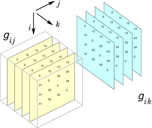
The objects with indices which would represent the and can be built from the matrices D as shown schematically in figure 1.
D3=zeros(N,N,N);
D3(:,:,:)  =  D2 (:,:,ones(N,1))
This corresponds to the first cube in figure 1, and it is going to be multiplied by a similar object obtained by permuting the indices as shown schematically in this listing:
D3=zeros(N,N,N);
D3(:,:,:)  =  D2 (:,:,ones(N,1)) ;
G1=gfun(D3);
G2=gfun(  permute ( D3, [ 1 3 2 ]  );
V3=  G1  .*  G2;
where the two matrices are multiplied element-wise.
5.3 Evaluation of the forces from SW potential
The total energy is sum over the triplets
but now the energies inside of the triplet must be specified. Since
With most reasonable interaction forms, where the first index specifies the “vertex of the ordered triplet”, in the specific case discussed, the atom where the bond angle is measured. For such cases the summation can run over all individual cases and results in
where now only factor 1/2 comes from the fact , i.e. the vertex is the same but the remaining pair ) can be counted twice. The evaluation of the forces is in principle identical, but can become quite different for cases where different degrees of simplification are possible.
For The SW case, the interactions can be described as pair-separable. For a given one has the form
| (26) |
Clearly, this form of interaction can be built as a three-index array, produced by element-wise multiplications of arrays constructed by duplication of matrices. Consider first a simpler form, where we keep just the funcions of distances,
The total energy three-index array
The notation is schematic, and shows that the total array be constructed as a product of two three index arrays each of which originates from replication of the original matrices. We introduce a symbol to denote the replication of matrix along the dimension which contains the number, while the dimensions marked by asterix appear once. Construction of the two arrays is shown in figure 1. We have also used the operator for element-wise multiplication of two arrays of the same dimensions in analogy with the MATLAB notation.
The importance of this is that also the gradient operations on such object will be obtained by operations on the original matrices, i.e. as . These are in form identical to the and so will be the . These gradients thus need to be calculated only for the matrix and replicated. Schematically we can write, following the above notation,
| (27) | |||||
Rewriting of these relations in the MATLAB notation will immediately produce the desired code. There will be a summation over two indices to produce the vector of forces from the three-index arrays. The evaluation of the gradients of the full SW-interaction follows in a straightforward manner the rules of chain derivative. The details and illustration of the evaluation of the gradient of the cosine is given in the appendix. Implementing the result shown in the appendix, we can also there apply the discussed fact that the term consists of pair-separable terms. Thus all the operations can be also there performed on matrices of distances and duplicated to the necessary three-index objects in precisely the same way as shown above for the distance functions. The only difference is that these are now Euclidian three dimensional vectors in addition to the particle-index dimensions. Thus the three-body forces can be constructed in a very similar way as the two-body forces. The computation is longer only due to the duplication of the matrices and element-wise products of the resulting matrices. The evaluation of the functional dependence does not change, since also here the computations are performed on matrices.
5.4 Symmetry aspects of 3-body force computations
The computations above can also be based on symmetry analysis. For a 3-body potential, each unique interacting triplet of particles has six different permutations contributing thus a total of six forces per index (particle). Since the Stillinger-Weber potential -formula , defined in eq. 23 - exhibits symmetry over the permutation of the second and third indices, i.e. , so that forces on the partilce satisfy
| (28) |
where the parenthesis denotes the particle coordinate of the gradient
| (29) |
Relations in eq. 28 demonstrate the symmetry of the problem and show that only three unique elements of the force array need to be computed for each particle in each triplet, as discussed also in other applications [6], [7]. Potential formula exhibits also the following antisymmetry due to the triplet’s geometrical configuration;
| (30) |
which can also be written as . Thus only two unique forces per particle per unique triplet are to be evaluated.
Computations of force arrays
Evaluation of analytical derivatives (gradients) of the 3-body term of the given potential with respect to the third index (along the fourth dimension), gives the array, which is denoted , holding the following six unique (two on each particle) force elements per triplet:
Those six unique force elements per triplet are what is needed to generate all the other elements by symmetry and antisymmetry exploitation. Transposing dimensions corresponding to the second and third indices of particles in array yields a new array , holding the other six force elements per triplet
The third array holding the last six force elements per triplet (cf. eq. 30)
is computed by the antisymmetry relation:
Finally the total force on -particle is a double sum over neighbors in triplets, i.e.
This will be done in array form by addition of arrays ,
[1 3 2 4]-permuted and
[1 4 3 2]-permuted (the permutation of array dimensions is done to place
the particle in the same position, see Appendix). The resulting 4-index array
and then summing over the third and fourth index of results in array of the forces.
Similar considerations and constructions can be done for the three-index arrays and their gradients in the case of Tersoff-type potentials in section 6 below, but there the symmetry and antisymmetry occur at two different stages of construction of the forces.
5.5 Experiments with three-body forces
In this section we have shown how one can use MATLAB functionality for evaluation of three body potentials and forces for three-body interactions. The operations on three-index arrays of the type discussed are ”expensive” in computer time but rather straightforward in terms of programming. The use of symmetries and more efficient build-up as discussed in sections 5.3 and 5.4 makes the computations much faster, but is much more error-prone. Here it can be useful to use a simple trick, formulate the computations first in a slow but easier programmed full-object version, even perhaps with the Kronnecker-deltas shown in eq. 15 implemented and explicitely summed, and then gradually introduce the more efficient computations in further versions. This offers possibilities for code development which are difficult to match in simplicity in other approaches. However, this approach offers even more benefits when investigating more complex interactions, as the Tersoff type discussed in the following section.
6 Tersoff-type many body potential
A more complex many-body potentials quite extensively used are the Tersoff type potentials. They are constructed in a slightly different way, but the techniques discussed in previous section can be used with some modifications also here. The many body character is introduced via a pair interaction, but the parameters of the interaction depend on the positions of the neigbours and the same bond angles for triplets formed by the pair and a neighbour atom. We first follow the formulation usually found in literature and later translate this to our notation. Considering a Morse-like potential, the energy can be written as a sum of cite energies as follows:
| (31) |
where
| (32) |
but where , i.e. their value is dependent on all the other particles, in practice on those which are in the neighborhood, as assured by the cut-off function. The function is an aproperiate cutoff function, while and are refered to as repulsive and attractive pair potentials respectively.
The two potential functions of the pair-wise interactions are:
| (33) |
The many-particle character in Tersoff’s formula is introduced by the following:
| (34) |
| (35) |
| (36) |
where is the angle between the and as defined above, and the set of parameters for carbon is given in [4]. In our work we used a Fermi-type cutoff function which has proven continuity and smoothness (infinitely differentiable) at any point,
where , and it is defined and parametrized in correspondence to that introduced by Tersoff [5], which has a different functional form but a very similar shape. Note that the same cut-off limits the pair interaction and the influence on the pair by the neighbors, the same appears both in eq. 33 and eq. 35.
To apply methods discussed in the previous section, we realize that the gradient operation can work on the various parts of the functional dependence. For simplicity, we omit the cut-off function in this discussion. The force on each particle is calculated by applying the the gradient
| (37) |
where we now re-write the above eqs. 31 to 36 in a more transparent notation
| (38) |
or
| (39) |
where
| (40) |
Applying the gradient,
| (41) |
we recognize that the first term is simply a two-body case discussed before. The really multi-body term is
| (42) |
The evaluation of the elements of matrices and as well as the function can be done in a straightforward way: construct the distance matrix as in eq 9, the unit vectors, and then construct the three-index array as in eq. 21, in MATLAB notation
Z=sum(Q,3);
produces the matrix Z.
We can treat all of the terms as before, except the
term
but we recognize that there is only one new typ of object,
| (43) |
but the has exactly the same form as the whole three-body contribution eq. 26 in the SW case and thus can be evaluated and reduced to a matrix in the same way as in the SW case. The difference is that it must be combined with the other terms above. In spite of its complicated formal nature the Tersoff-type potentials still contain only quantities including triplets of particles and the construction of the code is only a slightly more complex modification of the method outlined in section 5.2.
7 Conclusion
The discussed method, implementing multidimensional arrays along with their pre-defined operations, has proven to be a useful alternative to the standard loops aggregations in the vector-based MATLAB-like languages. It enables fast and powerful memory manipulations for interactive or exploratory work. In contrast to explicit loop programming it opens for speed-up and efficiency comparable to well optimized compiled arithmetic expressions in the framework of an interpreted code. Speed improvement is a main result of vectorized coding to which any numerical algorithm is very sensitive. Vectorization is known as performing operations on data stored as vectors, MATLAB stores matrices and arrays by columns in contiguous locations in the memory, and allows thus the use of vectorization on those objects. The elements of arrays can be selectively accessed in a vectorized fashion using so called logical indices. Mutidimensional logical arrays, as logical indices, have proven to be efficient and their use has resulted in a speed gain. Finally, the practicality, simplicity and generality of such a method to program empirical formulae for molecular dynamics purposes, make it effective to perform simulations on relatively small systems, up to 140 particles in a personal machine of 1 GB RAM, for Tersoff’s potential, a bigger system when using Stillinger-weber potential, and up to 1000 particles if only a pair interactions are used. The described methodology can be applied both to investigation of aspects of molecular dynamics and to educational purposes. Finally, programming in this method results in very short codes which are easily used and modified in interactive sessions.
Appendices
Appendix A Some aspects of MATLAB language
Matrix(Array) manipulation in MATLAB
-
Matrix(array) entering The lines starting with
>>are user input, the rest is matlab response. If input is ended by semicolon, no output follows.>> A= [ 1 4 5 2.5 7 ] A 1.0000 4.0000 5.0000 2.5000 7.0000 >> B= [ 1; 4; 2.5] B = 1.0000 4.0000 2.5000 >> C= [ 0 1 ; 1 0] C = 0 1 1 0 >> D=[ 1 4 3 5 2 3 7 6.6 2 2 ] D = 1.0000 4.0000 3.0000 5.0000 2.0000 3.0000 7.0000 6.6000 2.0000 2.0000The last example, matrix
Dshows multi-line possibility, the previous is a more compact matrix input. -
Accessing matrix(array) elements: Basic indexing
Assume
Ais a random 6 by 6 matrixA=rand(6,6)A([1 2 3],4)returns a column vector [ A(1,4) ; A(2,4) ; A(3,4) ]A(4,[1,1,1])returns a row vector [ A(4,1) A(4,1) A(4,1) ]A([2,5],[3,1])returns a 2 by 2 matrix [ A(2,3) A(2,1) ; A(5,3)A(5,1) ] -
Matrix(Array) size, length and number of dimensions:
The size of an array can be determined by the
size()command as :[nrows,ncols, npages, ....] = size(A)
where
nrows=size(A,1), ncols=size(A,2), npages=size(A,3)
This function is of much importance when aiming elements-wise operations as it is the key for arrays’ size matching.
The
ndims(A)function reports how many dimensions the arrayAhas. Trailing singleton dimensions are ignored but singleton dimensions occurring before non-singleton dimensions are not. This means thata=5; c=a(1,1); B=zeros(5,5); B(5,5,1)=4;
are valid expressions, even though they seemingly have non matching number of indices, but it is essential that the extra dimensions are ”singletons”, i.e. the extra dimensions have length one.
An interesting construction: one can construct matrices and arrays expanding the singleton dimensions.
a=5;   B=a([1 1],[1 1 1 1])
B =
     5     5     5     5
     5     5     5     5
The
length()command gives the number of elements in the longest dimension, and is equivalent tomax(size()). It is also used with a row or a column vector. -
Matrix(Array) replication:
One can use the MATLAB built-in script repmat, to replicate a matrix by the command:
repmat(A,[m n]), which replicates the matrixA(:,:)m-times in the first dimension (rows), and n-times in the second dimension (columns). This is a block matrix construction, the block corresponding to the original matrix A is repeated in a m n ”supermatrix”. The operation repmat is not a built-in but it is a script which means a slow execution. An alternative efficient way to achieve the same replication is by :A([1:size(A,1)]’*ones(1,m),[1:size(A,2)]’*ones(1,n))which is an application of basic indexing techniques.In this work we can use another aspect of
repmat()script, for building multidimensional arrays from matrices. Given a matrix A, its elements can be accessed byA(:,:), but that is equivalent toA(:,:,1), but alsoA(:,:,1,1), this is referred to as ”trailing singleton dimensions”. Using this, one can replicate the trailing dimensions. From an NN matrix we can construct a three-index NNN array byB=repmat(A,[1,1,N]);In the text we discuss a more efficient equivalentB=A(:,:,ones(1,N) ) -
Transpose and its generalization permute:
For a matrix (2D array) non-conjugate transpose is given by
transpose(A)and it is equivalent to a standard matrix operationA.’. The normal Hermite type conjugation is denoted byA’and has an equivalent functionctranspose(A). TheA.’-notation is somewhat surprising, since the dot usually denotes element-wise counterpart of the undotted operator (as e.g.A.^2, orA .* Betc).The generalizations of transpose-function to multi-dimensional arrays are given as
permute(A,ORDER)andipermute(A,ORDER)where ORDER means an array of reordered indeces. When ORDER is [1 2 3 4] for 4-index array, it means identity.transpose(A)andpermute(A,[2 1])give the same results as (A.’). The two permute-functions are related as shown in the exampleH=permute(G,[3,1,2]), G=ipermute(H,[3,1,2])If
size(G)is e.g.3 4 2thensize(H)is2 3 4Clearly, the inverse permute is introduced for convenience, the same result could be achieved by using the permute with appropriate order of dimensions.
-
Logical array addressing and predefined functions:
For a given matrix or array
Gthe functionlogical(G)returns an equal size array where there are logical ones (true) in elements which were nonzero and logical zeros (false) where the original array had zeros. ThusLg=logical(G)andLg=G>0both return the same matrix of logical ones and zeros.The extreme usefulness of these functions is that when we write
G(Lg)= 1 ./ G(Lg)the calculation will be performed only for the logically true addresses, thus no division by zero will happen. Or, we can ”shrink” a range of values; for example all values below a threshold can be given the threshold value and all values above a chosen top value can be given the top value. As an example, we take a matrix which should be modified by replacing all values smaller than 2 by 2 and all larger than 5 by 5. This can be done by the following commandsB=A; B(A>5) = A(A>5)*0+5; B(A<2) = A(A<2)*0+2The original matrix and the resulting one are
A=[ 1   5   3   6          B=  2   5   3   5
    7   3   1   1              5   3   2   2
    9   3   4   1              5   3   4   2
    3   4   2   1              3   4   2   2
    9   2   3   1 ]            5   2   3   2
There are also available functions analogous to
ones( )andzeros( ). As an example,false(5,2,2)returns the same logical array aszeros(5,2,2)>0andtrue(5,2,2)is the same as e.g.logical(ones(5,2,2))The use of logical addressing can shorten some large array manipulations and calculations, but also consumes some processing time.
One can test the gains and losses by filling a large array and doing the element-wise operations on the whole array and the logically addressed part of the array.
In this example we show the array of ten million numbers, where only 100 are nonzero.
N =  10000000;
octave >  tic;  C=zeros(N,1);  C(100:200)=1;  D=exp(C);  toc
     Elapsed time is 0.601 seconds.

octave > tic;C=zeros(N,1);C(100:200)=1;    D(C>0)=exp(C(C>0));toc
     Elapsed time is 0.394 seconds.
In the second line we have calculated only the nonzero cases using the discussed logical addressing. We observe that there is a certain small gain in time, but far under the factor expected from the number of calculations. It should also be mentioned that the return times are not reproduceable, they depend on the over all state of the computer memory.
Speed improvement in Matlab
-
Array Preallocation :
Matlabs matrix variables dynamically augment rows and columns and the matrix is automatically resized. Internally, the matrix data memory must be reallocated with larger size. If a matrix is resized repeatedly like within a for loop, this overhead becomes noticeable. When a loop is of a must demand, as the inevitable time-loop in MD programs, frequent reallocations are avoided by preallocating the array with one of thezeros(),ones(),rand(),true()andfalse()commands. -
Vectorization of MATLAB’s computation and logical addressing: Vectorized computations which mean replacing parallel operations, i.e., simultaneous execution of those operations in loops, with vector operations, improves the speed often ten-fold. For that purpose, most standard functions in Matlab are vectorized, i.e., they operate on an array as if the function was applied individually to every element. Logical addressing operations are also vectorized, the use of logical addressing may lead to vectorized computations only for elements where the indices are true, thus reducing execution time, in some cases substantially.
Appendix B Gradient of the cosine of the bond angle for three body forces
Let a, b and c mark three atoms, the b-atom is at the vertex of the angle ;
Define the following quantities:
; ;
;
![[Uncaptioned image]](/html/0908.1561/assets/x2.png)
Gradient with respect to the end
| (44) |
Gradient with respect to the end
| (45) |
gradient with respect to point ’b’ :
| (46) |
The gradients satisfy the following relation
| (47) |
which simply confirms the fact that moving the vertex point by a vector is the same as moving each of the end points and simultaneously by the vector .
Derivation:
In view of eq. 47 it is necessary to evaluate just one endpoint, the second follows from symmetry and the vertex is given by relation eq. 47
The calculation is done by using
| (48) |
and
| (49) |
Applying these two to the chain derivatives in the gradient as
References
-
[1]
http://web.ift.uib.no/AMOS/matlab_md/ -
[2]
Peter J. Acklam.
Matlab array manipulation tips and tricks.
Oct 2003.
http://home.online.no/~pjacklam/matlab/doc/mtt/index.html - [3] Frank H. Stillinger and Thomas A. Weber. Computer simulation of local order in condensed phases of silicon. Phys. Rev. B, 31(8):5262–5271, Apr 1985.
- [4] J. Tersoff. Empirical interatomic potential for carbon, with applications to amorphous carbon. Phys. Rev. Lett., 61(25):2879–2882, Dec 1988.
- [5] J. Tersoff. New empirical approach for the structure and energy of covalent systems. Phys. Rev. B, 37(12):6991–7000, Apr 1988.
- [6] J. V. Sumanth, David R. Swanson, and Hong Jiang. A symmetric transformation for 3-body potential molecular dynamics using force-decomposition in a heterogeneous distributed environment. In ICS ’07: Proceedings of the 21st annual international conference on Supercomputing, pages 105–115, New York, NY, USA, 2007. ACM.
- [7] Jianhui Li, Zhongwu Zhou, and Richard J. Sadus. Modified force decomposition algorithms for calculating three-body interactions via molecular dynamics. Computer Physics Communications, 175(11-12):683 – 691, 2006.