Steady-State Two Atom Entanglement in a Pumped Cavity

Abstract

In this paper we explore the possibility of a steady-state entanglement of two two-level atoms inside a pumped cavity by taking into account cavity leakage and the spontaneous emission of photons by the atoms. We describe the system in the dressed state picture in which the coherence is built into the dressed states while transitions between the dressed states are incoherent. Our model assumes the vacuum Rabi splitting of the dressed states to be much larger than any of the decay parameters of the system which allows atom-field coherence to build up before any decay process takes over. We show that, under our model, a pumping field cannot entangle two closed two-level atoms inside the cavity in the steady-state, but a steady-state entanglement can be achieved with two open two-level atoms.

I Introduction

In this paper we investigate the steady-state entanglement of two two-level atoms inside a high-Q cavity which is pumped by an external field. We assume a large vacuum Rabi splitting, and take into account the presence of cavity leakage and spontaneous emission by the atoms. We demonstrate that a pumping field cannot entangle two two-level atoms inside a cavity in the steady-state, but it is possible to have steady state entanglement between two open two-level atoms in a cavity in the presence of a pumping field. This is achieved by optically pumping half of the atomic population outside of the decoherence-free subspace of the system, and the process yields an entanglement equivalent to a Bell state content of $\frac{1}{2}$.

Entanglement between two partitions of a system is often due to some constraint placed on the dynamics of the system. This constraint can take the form of energy conservation, momentum conservation, or structural constraint to name a few. In this paper we direct our attention to the entanglement that arises from the constraints on the energy, or more specifically, the number of excitations in our system.

In a simple system of two two-level atoms inside a cavity, initially in their ground states, and with one photon in the cavity mode, we know that the two atoms get entangled and disentangled periodically in time. This could lead one to think that if the two atoms were placed in a sufficiently high-Q cavity with small losses introduced and externally pumped such that the average photon number in the cavity is less than or equal to one, then the two atoms would still get entangled in some fashion. In the simplest case in which one pumps the cavity with a single photon source, and constrains the pumping rate to be less than or equal to the decay rate of the system, it would seem plausible that the two atoms inside the cavity can be entangled. In fact, making a weak field assumption and only taking into account the first order correction to the reduced density matrix of the atoms will yield a non-zero entanglement between the atoms. However, we show that if one were to take into account the higher order corrections in the density matrix, then the entanglement between the atoms vanish. The result is due to the fact that the concurrence measure is a nonlinear function of the parameters of the atomic density matrix. The weak field assumption is only valid if one is calculating some property of the atoms which is linearly dependent on the parameters.

Recent experimental advances in atomic traps and cavity QED Wienman ; Wineland ; Haroche ; Walther ; Kimble offer exciting new possibilities in quantum computation and quantum networking using the entanglement between atoms in the cavity Walther2 . It is within our technological limits to trap and manipulate atoms inside a microcavity to study their entanglement behavior Haroche . Therefore, it is important to characterize the entanglement of the atoms in the cavity, and how the entanglement is changed by the dynamics of the system.

Theoretical work on atoms inside a cavity Guo ; Li ; Orozco ; Knight suggests not only entanglement between atoms in a cavity, but the possibility of a steady-state atomic entanglement in presence of a weak pump. Here we will investigate under what circumstances the atoms inside the cavity will get entangled with each other, and whether a steady-state entanglement can be attained.

Our approach to characterizing the entanglement between atoms inside a cavity is through the dressed state picture of the atom-field states in the limit of large vacuum Rabi splitting. This approach enables us to use rate equations to characterize the transitions between the dressed states Tan1 ; Stroud . All the coherent effects are contained within the dressed states, and the transitions between the dressed levels are incoherent effects which are attributed to spontaneous decay of the atom, cavity leakage, or pumping. Also, for simplicity, we ignore longitudinal dipole-dipole interaction between the atoms and motional effects in our calculation. The advantage to our approach, which expresses the density matrix of the system as a mixture of the dressed states, is that we can identify which dressed states contribute to the entanglement between the atoms. This will more directly suggest how one may manipulate the system in order to maximize entanglement between the atoms. We will show that in the steady-state regime a pumping field cannot entangle two closed two-level atoms in the steady-state, but it is possible to entangle two open two-level atoms in the steady-state with an entanglement content worth one half a Bell state through optically pumping atomic population out of the decoherence-free subspace of the system using a pumping field.

First, we will investigate the case in which two closed two-level atoms are inside a cavity by taking into account the $n=0$, $n=1$, and $n=2$ dressed states, and we show there is no entanglement between the atoms. Then we will show that a calculation involving only the $n=0$ and $n=1$ dressed states yield a non-zero entanglement between the atoms. Although this approach is reasonable for weak pumping fields when one is seeking the density matrix for the purpose of determining the population distribution, or other characteristics of the atoms which depend linearly on the density matrix, we will show that taking into account only the $n=1$ dressed states is insufficient for the purposes of determining the entanglement between the atoms. We then proceed to show that a steady-state entanglement can be obtained in the presence of a pumping field for the case of two open two-level atoms even when we consider all the dressed states of the system.

II Model System: Two Closed Two-level Atoms Inside a Cavity

II.1 Multiple Excitation in the Cavity

In this section we will show that a pumping field cannot generate entanglement between two two-level atoms inside a high-Q cavity in the presence of cavity leakage and spontaneous emission by the atoms. The atoms are both initially in the ground state, and they are placed in the cavity with the cavity mode being on resonance with the atomic transition. The external pumping field is also on resonance with the atomic transition in our model. Furthermore, to be consistent with the high-Q cavity assumption, we will stipulate that the Rabi splitting is much larger than the spontaneous decay rate and the cavity leakage rate. The large Rabi splitting justifies the rate equation approach we will take to analyze our system.

The system we are considering consists of two atoms, each with energy structure shown in Fig.(1), in a cavity which is externally pumped on resonance with the atomic transition. The system can lose energy through cavity leakage or through spontaneous emission of the atoms.

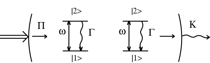
Figure 1: Two closed two-level atoms inside a cavity

Since we wish to characterize this system using rate equations, we will first obtain the dressed states of the closed system, and later calculate the transition rates between these dressed states. We assume that the Rabi splitting in this system is large such that the coherence of the atoms and the field is contained in the dressed states. Therefore, pumping population from the ground state up to these dressed states results in populating an incoherent mixture of these dressed states. We will study the entanglement between the atoms in the steady-state regime after we obtain the rate equations that govern the population distribution of the system.

The Hamiltonian of the closed system in the interaction picture is

$$\hat{H}_{I}=g_{1}\hat{\sigma}_{12}^{(1)}\hat{a}^{\dagger}+g_{2}\hat{\sigma}_{12}^{(2)}\hat{a}^{\dagger}+H.C.$$ (1)

where $\hat{\sigma}_{ij}^{(n)}$ is the atomic transition operator for the $n^{th}$ atom and $\hat{a}^{\dagger}$ is the field creation operator. For the sake of simplicity we will assume the coupling constants, $g_{i}$, to be the same for each atom. In the case in which there is only one excitation in the system there are three essential states,

$$\begin{array}[]{l}|11;1\rangle\\ |12;0\rangle\\ |21;0\rangle,\\ \end{array}$$ (2)

and three dressed states,

$$|\chi_{o}\rangle=\frac{1}{\sqrt{2}}\big{(}|12;0\rangle-|21;0\rangle\big{)},$$ (3)

$$|\chi_{+}\rangle=\frac{1}{\sqrt{2}}|11;1\rangle+\frac{1}{2}\big{(}|12;0\rangle+|21;0\rangle\big{)},$$ (4)

$$|\chi_{-}\rangle=\frac{1}{\sqrt{2}}|11;1\rangle-\frac{1}{2}\big{(}|12;0\rangle+|21;0\rangle\big{)}.$$ (5)

Here $|ab;c\rangle=|a\rangle_{1}\otimes|b\rangle_{2}\otimes|c\rangle_{f}$ indicates the first atom is in state $|a\rangle$, the second atom in state $|b\rangle$, and the field in state $|c\rangle$.

In order to construct the rate equations governing the distribution of the populations we will now need to calculate the spontaneous emission rate, pumping rate, and the cavity leakage rate of the system. The spontaneous emission rate between states $|a\rangle$ and $|b\rangle$ is proportional to $|\langle a|\hat{d}_{ab}|b\rangle|^{2}$ where $\hat{d}_{ab}$ is the dipole matrix element between states $|a\rangle$ and $|b\rangle$. Therefore, the rate of decay of the dressed states into the ground state, $|g\rangle=|11;0\rangle$, is given by,

$$\begin{array}[]{l}\gamma_{o\rightarrow g}=\Gamma|\langle\chi_{o}|\hat{d}^{(1)}+\hat{d}^{(2)}|g\rangle|^{2}=0,\\ \gamma_{+\rightarrow g}=\Gamma|\langle\chi_{+}|\hat{d}^{(1)}+\hat{d}^{(2)}|g\rangle|^{2}=\Gamma,\\ \gamma_{-\rightarrow g}=\Gamma|\langle\chi_{-}|\hat{d}^{(1)}+\hat{d}^{(2)}|g\rangle|^{2}=\Gamma,\end{array}$$ (6)

where $\Gamma$ is the Einstein A coefficient of the $2\rightarrow 1$ transition of the single atom in free space.

Likewise, the pumping rate of the cavity is proportional to $|\langle c|\hat{a}^{\dagger}|c-1\rangle|^{2}$, where $|c\rangle$ is the field state in the Fock basis. The pumping rates for the dressed states from the ground state is given by,

$$\begin{array}[]{l}\pi_{g\rightarrow o}=\Pi|\langle\chi_{o}|\hat{a}^{\dagger}|g\rangle|^{2}=0,\\ \pi_{g\rightarrow+}=\Pi|\langle\chi_{+}|\hat{a}^{\dagger}|g\rangle|^{2}=\frac{\Pi}{2},\\ \pi_{g\rightarrow-}=\Pi|\langle\chi_{-}|\hat{a}^{\dagger}|g\rangle|^{2}=\frac{\Pi}{2},\end{array}$$ (7)

where $\Pi$ is the single photon pumping rate inside the cavity (i.e. $\Pi=\Pi_{source}T^{2}$ where $T$ is the amplitude transmission coefficient of the input cavity mirror and $\Pi_{source}$ is the single photon emission rate of the pumping source).

The cavity leakage rate is obtained in a similar fashion,

$$\begin{array}[]{l}\kappa_{o\rightarrow g}=K|\langle\chi_{o}|\hat{a}^{\dagger}|g\rangle|^{2}=0,\\ \kappa_{+\rightarrow g}=K|\langle\chi_{+}|\hat{a}^{\dagger}|g\rangle|^{2}=\frac{K}{2},\\ \kappa_{-\rightarrow g}=K|\langle\chi_{-}|\hat{a}^{\dagger}|g\rangle|^{2}=\frac{K}{2}.\end{array}$$ (8)

Here $K$ is the power transmission coefficient of the cavity output mirror.

The $n\geq 2$ excitation of the system will have a different set of dressed states since there are four essential states in this case. The four essential states for $n\geq 2$ are,

$$\begin{array}[]{l}|11;n\rangle\\ |12;n-1\rangle\\ |21;n-1\rangle,\\ |22;n-2\rangle.\\ \end{array}$$ (9)

The dressed states are then given by,

$$|\phi_{o}^{n}\rangle=\frac{1}{\sqrt{2}}\big{(}|12;n-1\rangle-|21;n-1\rangle\big{)},$$ (10)

$$|\phi_{o^{\prime}}^{n}\rangle=\frac{1}{\sqrt{2}}\big{(}|11;n\rangle-|22;n-2\rangle\big{)},$$ (11)

$$|\phi_{+}^{n}\rangle=\frac{1}{2}\big{(}|11;n\rangle+|12;n-1\rangle+|21;n-1\rangle+|22;n-2\rangle\big{)},$$ (12)

$$|\phi_{-}^{n}\rangle=\frac{1}{2}\big{(}|11;n\rangle-|12;n-1\rangle-|21;n-1\rangle+|22;n-2\rangle\big{)}.$$ (13)

After we calculate the pumping rate, cavity leakage rate, and spontaneous emission rate by the atoms between the dressed states, as we have done before for the $n=1$ dressed states and the ground state, we can construct the rate equation governing the population distribution amongst the $n=0$, $n=1$, and $n=2$ dressed states. The rate equation is given by,

$$\begin{array}[]{l}\dot{P}_{g}=\Gamma P_{s1}+\frac{K}{2}P_{s1}-\Pi P_{g},\\ \dot{P}_{s1}=-\Gamma P_{s1}-\frac{K}{2}P_{s1}+\Pi P_{g}+\frac{3}{2}\Gamma P_{s2}+\Gamma P_{o^{\prime},2}+K(P_{s2}+P_{o^{\prime},2})+\frac{3}{2}\Pi P_{s1},\\ \dot{P}_{s2}=-\frac{3}{2}\Gamma P_{s2}-KP_{s2}+\Pi P_{s1},\\ \dot{P}_{o^{\prime},2}=-\Gamma P_{o^{\prime},2}-KP_{o^{\prime}}+\frac{1}{2}\Pi P_{s1},\\ \dot{P}_{o}=0,\\ \dot{P}_{o,2}=0,\\ P_{s1}=P_{+}+P_{-},\\ P_{s2}=P_{+,2}+P_{-,2},\end{array}$$ (14)

where $P_{g}$ is the population of the ground state of the system, $P_{\pm}$ is the population in the $|\chi_{\pm}\rangle$ dressed states, $P_{0}$ is the population in the $|\chi_{o}\rangle$ dressed state, $P_{\pm,n}$ is the population in $|\phi_{\pm}^{n}\rangle$, $P_{o,n}$ is the population in the $|\phi_{o}^{n}\rangle$, and $P_{o^{\prime},n}$ is the population in $|\phi_{o^{\prime}}^{n}\rangle$. Here we assume that there is no population initially in the $|\chi_{o}\rangle$ and $|\phi_{o}^{n}\rangle$ dressed states, and because these states don’t couple to any other states, they will not accumulate any population at later times.

The steady-state solution to these rate equations is,

$$\begin{array}[]{l}P_{g}=\mathcal{N}(3\Gamma+2K)(2\Gamma+K)(\Gamma+K),\\ P_{s1}=\mathcal{N}2\Pi(\Gamma+K)(3\Gamma+2K),\\ P_{s2}=\mathcal{N}4\Pi^{2}(\Gamma+K),\\ P_{o^{\prime},2}=\mathcal{N}\Pi^{2}(3\Gamma+2K),\\ \mathcal{N}=7\Gamma\Pi^{2}+6\Pi^{2}K+6\Pi\Gamma^{2}+10\Pi K\Gamma+4\Pi K^{2}+6\Gamma^{3}+13K\Gamma^{2}+9K^{2}\Gamma+2K^{3}.\\ \end{array}$$ (15)

Are the two atoms in the cavity entangled? In order to answer this question we will have to calculate the entanglement content of this bipartite two-level mixed state of the system. Here we will employ the concurrence measure put forward by Wootters wooters . The concurrence measure of entanglement is defined as,

$$C=max(\sqrt{\lambda_{1}}-\sqrt{\lambda_{2}}-\sqrt{\lambda_{3}}-\sqrt{\lambda_{4}},0)$$ (16)

where $\lambda_{i}$ are the eigenvalues, in descending order of value, of the matrix $\rho\tilde{\rho}$ ($\tilde{\rho}=(\sigma_{y}\otimes\sigma_{y})\rho^{*}(\sigma_{y}\otimes\sigma_{y})$).

To determine the entanglement between the atoms in the cavity we will trace out the field component of the density matrix to obtain the reduced density matrix of the system. The reduced density matrix of the two atoms is given by,

$$\hat{\rho}_{atoms}=P_{g}\hat{\rho}_{g}+P_{s1}\hat{\rho}_{s1}+P_{s2}\hat{\rho}_{s2}+P_{o^{\prime},2}\hat{\rho}_{o^{\prime},2}$$ (17)

where

$$\hat{\rho}_{g}=\begin{pmatrix}1&0&0&0\\ 0&0&0&0\\ 0&0&0&0\\ 0&0&0&0\\ \end{pmatrix},\hat{\rho}_{s1}=\begin{pmatrix}\frac{1}{2}&0&0&0\\ 0&\frac{1}{4}&\frac{1}{4}&0\\ 0&\frac{1}{4}&\frac{1}{4}&0\\ 0&0&0&0\\ \end{pmatrix},\hat{\rho}_{s2}=\begin{pmatrix}\frac{1}{4}&0&0&0\\ 0&\frac{1}{4}&\frac{1}{4}&0\\ 0&\frac{1}{4}&\frac{1}{4}&0\\ 0&0&0&\frac{1}{4}\\ \end{pmatrix},\hat{\rho}_{o^{\prime},2}=\begin{pmatrix}\frac{1}{2}&0&0&0\\ 0&0&0&0\\ 0&0&0&0\\ 0&0&0&\frac{1}{2}\\ \end{pmatrix}.$$ (18)

The important point to note in the dressed states for $n\geq 2$ is that, aside from the $|\phi_{o}^{n}\rangle$ which does not couple to any of the other dressed states through spontaneous emission, pumping, or leakage, the other three dressed $|\phi_{o^{\prime}}^{n}\rangle$, $|\phi_{+}^{n}\rangle$, and, $|\phi_{-}^{n}\rangle$ have no entanglement (i.e $C=0$) between the atoms. This is in contrast with the $n=1$ dressed states, $|\chi_{\pm}\rangle$, which does contain entanglement between the two atoms ($C=\frac{1}{2}$). This suggests that any strong pumping which puts appreciable population in the $n\geq 2$ will disentangle the atoms. On the other hand, it may seem to suggest that in the limit of weak pumping, in which the $n\geq 2$ dressed states are not appreciably populated, the atoms may turn out entangled. We will show that the atoms do not get entangled no matter how weak the pumping field.

The concurrence of $\hat{\rho}_{atoms}$ is,

$$C_{atoms}=max\big{(}\frac{1}{2}(P_{s1}+P_{s2})-\frac{1}{2}\sqrt{(P_{s2}+2P_{o^{\prime},2})(2P_{o^{\prime},2}+P_{s2}+4P_{g}+2P_{s1})},0\big{)}.$$ (19)

It is not easy to determine by observation if there exists some combination of parameters which would provide a non-zero concurrence. The plot of the expressions inside the $max$ function of the concurrence (which we will call $\mathcal{C}$) against $\Pi$ and $K$ (in units of $\Gamma$) Fig. (2) suggests that there is indeed no combination of parameters which will provide a non-zero entanglement content.

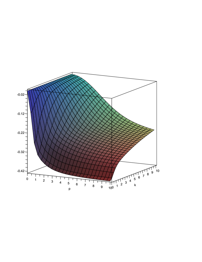
Figure 2: Plot of $\mathcal{C}$ against $\Pi$ and $K$ (in units of $\Gamma$)

Can there be a miniscule amount of entanglement that we don’t see in the plot? In order to answer this let us take a closer look at the expression for concurrence. First, we will determine if there are any extremums in the expression for concurrence by looking at the partial derivatives of $C$ with respect to the $P_{i}$ parameters and setting the expression to zero. After differentiating C we obtain,

$$\begin{array}[]{l}\frac{\partial C}{\partial P_{g}}=-\frac{\mathcal{A}}{4}(8P_{o^{\prime},2}+4P_{s2})=0,\\ \frac{\partial C}{\partial P_{s1}}=\frac{1}{2}-\frac{\mathcal{A}}{4}(4P_{o^{\prime},2}+2P_{s2})=0,\\ \frac{\partial C}{\partial P_{s2}}=\frac{1}{2}-\frac{\mathcal{A}}{4}(4P_{g}+2P_{s1}+2P_{s2}+4P_{o^{\prime},2})=0,\\ \frac{\partial C}{\partial P_{o^{\prime},2}}=-\frac{\mathcal{A}}{4}(4P_{s2}+8P_{g}+4P_{s1}+8P_{o^{\prime},2})=0,\\ \mathcal{A}=\frac{1}{\sqrt{4P_{s2}P_{g}+2P_{s1}P_{s2}+P_{s2}^{2}+4P_{s2}P_{o^{\prime},2}+8P_{o^{\prime},2}P_{g}+4P_{o^{\prime},2}P_{s1}+4P_{o^{\prime},2}^{2}}}.\end{array}$$ (20)

It is easy to see that $\frac{\partial C}{\partial P_{g}}=0$ and $\frac{\partial C}{\partial P_{o^{\prime},2}}=0$ cannot be satisfied by positive real values of the $P_{i}$. The $P_{i}$ have to be positive real values since they are the probability weighting of the density matrix, and the steady-state solution suggests a non-zero value for all the $P_{i}$. The $\frac{\partial C}{\partial P_{s1}}=0$ and $\frac{\partial C}{\partial P_{s2}}=0$ takes some algebra, but one can also show that the equations cannot be satisfied within the restrictions of the parameters. Therefore, there are no extrema or saddle points in the concurrence, which is consistent with Fig. (2). This means that the extremum value lies on the boundary of the domain of the $P_{i}$. The four boundary points are $(P_{g}=1,P_{s1}=0,P_{s2}=0,P_{o^{\prime},2}=0)$, $(P_{g}=0,P_{s1}=1,P_{s2}=0,P_{o^{\prime},2}=0)$, $(P_{g}=0,P_{s1}=0,P_{s2}=1,P_{o^{\prime},2}=0)$, and $(P_{g}=0,P_{s1}=0,P_{s2}=0,P_{o^{\prime},2}=1)$, of which only the $(P_{g}=0,P_{s1}=1,P_{s2}=0,P_{o^{\prime},2}=0)$ point offers a nonzero concurrence of $C=\frac{1}{2}$. Hence, the only possible non-zero value of the concurrence is along the $P_{s1}$ axis from $(P_{g}=0,P_{s1}=1,P_{s2}=0,P_{o^{\prime},2}=0)$. Our task is to determine the maximum value of $P_{s1}$ constrained by the steady-state solutions to the rate equations.

Using numerical techniques one can determine the maximum value of $P_{s1}$ to be $P_{s1}\approx 0.366$ which implies $P_{g}\approx 0.317$, $P_{s2}\approx 0.211$, and $P_{o^{\prime},2}\approx 0.106$ (see Fig. (3)). These population yields a concurrence of $C=max(\sqrt{(}0.083)-2\sqrt{(}0.0640),0)=0$. This means that a pumping field that takes any population beyond the $n=1$ dressed state leaves the atoms completely unentangled.

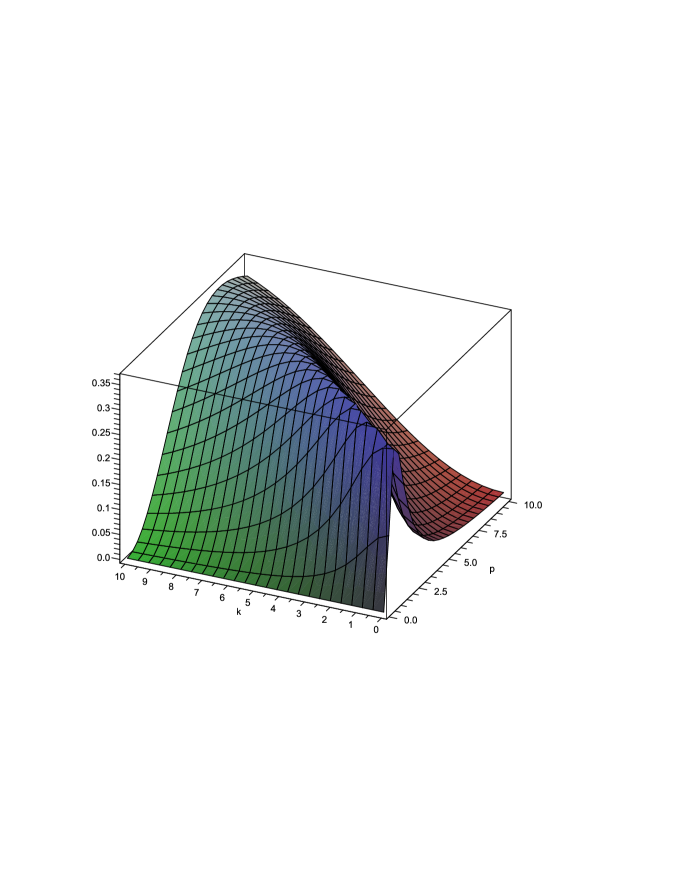
Figure 3: Plot of $P_{s1}$ against $\Pi$ and $K$ (in units of $\Gamma$)

There are a couple points here worth noting. First, we only extended the rate equations to include the $n=2$ dressed states, and yet the concurrence suddenly dropped to zero. In reality, the $n>2$ dressed states do get populated as well, so as far as the entanglement of the atoms are concerned we are actually overestimating the concurrence. This is because in reality only some fraction of that population resides in the $n=2$ states and the rest is somewhere in the $n>2$ dressed states. Therefore, this implies even less population in the $|\chi_{\pm}\rangle$ dressed states, and, as a consequence, less entanglement between the atoms. Second, we would expect that in the limit of a weak pump the $n=2$ dressed states would not get appreciably populated, so the entanglement between the atoms ought to be non-zero. However, our analysis indicates that any population at all in the $n=2$ dressed states disentangles the atoms. Lets take a numerical example to illustrate this peculiar point. For $\Pi=.447$ and $K=1$ (in units of $\Gamma)$ we get $P_{g}=0.97337$, $P_{s1}=0.02595$, $P_{s2}=0.00042$, and $P_{o^{\prime},2}=0.00026$. One would be tempted to neglect the $P_{s2}$ and $P_{o^{\prime}2}$ terms in the density matrix since they are two orders of magnitude smaller than $P_{s1}$. If we only keep the leading two terms then we get a concurrence of $C=.01$. However, if we were to keep all the terms in the density matrix we would get a concurrence of $C=0$. Although $P_{s2}$ and $P_{o^{\prime}2}$ were two orders of magnitude smaller, by keeping these terms in the density matrix we see there is no entanglement between the atoms. In principle, we can always extend the accuracy of our model by increasing the Rabi splitting of the dressed states. Therefore, the miniscule population in $n=2$ disentangling the atoms is indeed the case for the model we are considering. Because concurrence is not necessarily linear in the parameters of the density matrix, one cannot ignore terms even when they are several orders of magnitude smaller. In order to get a non-zero entanglement between the atoms we have to put more population in the $|\chi_{\pm}\rangle$ dressed states, and minimize the population transfer to the $n\geq 2$ dressed states. The only realistic option we have is to have cavity leakage rate that is nonlinear in the photon number Gaeta ; Stank since $\Gamma$ is a fixed parameter of the atoms and $\Pi$ is a pumping parameter that does not differentiate between the cavity field excitation number. If the mirror of the cavity demonstrates a strong enough nonlinearity between the one excitation and two excitation of the cavity field then one can obtain a non-zero concurrence between the two atoms.

Finally, we would like to offer a more intuitive justification for our use of the rate equations. Clearly, the way we construct the rate equations suggests that the populations of the dressed states depends only on the populations of the other dressed states and not the coherence between the dressed states. The downward transitions, spontaneous emission of the atoms and cavity decay, are incoherent processes, so they do not impart any coherence onto the system. The upward transition, the external pumping, also does not impart any coherence in the steady-state limit. When a photon impinges on an atom initially in the ground state inside a cavity, the system is put in a coherent superposition of the dressed states whose amplitudes oscillate with the associated Rabi frequency. However, when a decay process is introduced, the atom-cavity system can lose the photon and go back into the ground state. At this point they wait for the next pump photon to come and restart the Rabi oscillation. In effect, the quantum jump that is introduced randomizes the initial phase of the dressed states Rabi oscillation. We do not know when the photon was lost nor do we know when the new pump photon has arrived. Therefore, in the longtime limit, after many decay and pumping processes have taken place, we do not expect to have any coherence between the dressed states since we will have no information concerning the phase of the Rabi oscillation. For this reason we can use rate equations to describe our system.

II.2 Single Excitation in the Cavity

In the previous section we demonstrated that a pumping field cannot entangle the atoms in the steady-state inside the cavity under our model. In this section we will briefly exam what one might obtain for the entanglement between the atoms if one employs the weak field assumption and decides to only consider the $n=1$ dressed states. The model seems plausible in the limit of a weak pumping field, but we will show how the weak pumping assumption does not translate to only considering the $n=1$ dressed states.

If one were to consider only the $n=1$ dressed states then the rate equation governing the population distribution given by,

$$\begin{array}[]{l}\dot{P}_{g}=\Gamma(P_{+}+P_{-})+\frac{K}{2}(P_{+}+P_{-})-\Pi P_{g},\\ \dot{P}_{o}=0,\\ \dot{P}_{+}=-\Gamma P_{+}-\frac{K}{2}P_{+}+\frac{\Pi}{2}P_{g},\\ \dot{P}_{-}=-\Gamma P_{-}-\frac{K}{2}P_{-}+\frac{\Pi}{2}P_{g}.\\ \end{array}$$ (21)

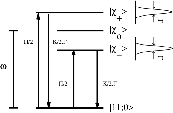
Figure 4: Schematic of the dressed state

Provided there is no population in $P_{o}$ at $t=0$, the steady-state solution of these equations is,

$$\begin{array}[]{l}P_{+}=P_{-}=N\frac{\Pi}{2},\\ P_{g}=N(\frac{K}{2}+\Gamma),\\ N=\frac{1}{\Gamma+\frac{K}{2}+\Pi}.\end{array}$$ (22)

The total density matrix (including the two atoms and the field) is given by,

$$\hat{\rho}=P_{g}|g\rangle\langle g|+P_{+}|\chi_{+}\rangle\langle\chi_{+}|+P_{-}|\chi_{-}\rangle\langle\chi_{-}|+P_{o}|\chi_{o}\rangle\langle\chi_{o}|.$$ (23)

Since we are only interested in the entanglement between the two atoms, we will trace out the field part of the density matrix to obtain the reduced density matrix for the two atoms. This is given by,

$$Tr_{field}(\hat{\rho})=\big{(}P_{g}+\frac{1}{2}(P_{+}+P_{-})\big{)}|11\rangle\langle 11|+\frac{1}{2}(P_{+}+P_{-})|\psi^{+}\rangle\langle\psi^{+}|+P_{o}|\psi^{-}\rangle\langle\psi^{-}|$$ (24)

where $|\psi^{+}\rangle=\frac{1}{\sqrt{2}}\big{(}|12\rangle+|21\rangle\big{)}$ and $|\psi^{-}\rangle=\frac{1}{\sqrt{2}}\big{(}|12\rangle-|21\rangle\big{)}$ are the two Bell states. Substituting our previous steady-state solution to the above equation yields,

$$\hat{\rho}_{atoms}=N\big{[}(\frac{\Pi+K}{2}+\Gamma)|11\rangle\langle 11|+\frac{\Pi}{2}|\psi^{+}\rangle\langle\psi^{+}|\big{]}.$$ (25)

The concurrence for this reduced density matrix is simply $C=N\frac{\Pi}{2}$. This model suggests that whenever the pump is on there is always some entanglement between the atoms inside the cavity. This result is contrary to the one we have obtained earlier. If we only consider the $n=1$ dressed states, then there is always some entanglement between the two atoms in the steady-state when the pump is on. However, we have shown earlier that, no matter how weak the pumping field, the two atoms do not get entangled in the steady-state. The discrepancy between the two results is due to the fact that concurrence is not a linear function of the density matrix. If concurrence were linearly related to the density matrix, then the weak field assumption would be valid, and the two atoms would indeed be entangled. But because concurrence is not a linear function of the density matrix (or, the wave function of the system), one cannot dismiss the $n\geq 2$ terms in the density matrix even when the population in those states are significantly smaller than the $n=1$ and $n=0$ dressed states. Therefore, the weak field assumption does not translate to just keeping the lowest order terms in the density matrix if one is interested in calculating the entanglement content of a system.

In our analysis we have assumed that the atoms were on resonance with the cavity field mode and the coupling constants of the atoms were the same. If the atoms had a different coupling constant $g_{i}$, or detuned from the cavity field by $\Delta_{i}$, this would result in the reduction of the entanglement between the atoms. The entanglement between the atoms here is due to the $|\psi^{+}\rangle$ in the $|\chi_{\pm}\rangle$ dressed states. Different coupling constants or detuning would turn the $|\psi^{+}\rangle$ into $\frac{1}{\sqrt{|\alpha|^{2}+|\beta|^{2}}}\big{(}\alpha|12\rangle+\beta|21\rangle\big{)}$ in the dressed states, and in general, $\alpha\neq\beta$. Because maximum entanglement is attained when $\alpha=\beta=\frac{1}{\sqrt{2}}$, the effect of differing $g_{i}$’s or $\Delta_{i}$’s would reduce the entanglement between the atoms. Therefore, the case we are considering is the case for maximum possible entanglement between the atoms.

III Model System: Two Open Two-level Atoms Inside a Cavity

So, is there a way to generate steady-state entanglement with pumping/leakage through the cavity and spontaneous emission? Indeed there is a way to generate entanglement under these conditions using two open two-level atoms. The system we consider, Fig.(5), is two open two-level atoms inside a cavity with spontaneous emission down to both ground states and the cavity being in resonance with only one transition of the open two-level atom.

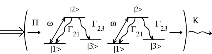
Figure 5: Two open two-level atoms inside a cavity

Since the pumping field does not interact with $|3\rangle$, the Hamiltonian of the closed system is the same as the two closed two-level system model, and therefore the dressed states are also the same. The only difference is that when we construct our rate equations we have the possibility of the atom to fall into the $|3\rangle$ state through spontaneous emission.

Now, if we were to start out in the $|11;0\rangle$ state as we did before then we will get no entanglement between the atoms since the $|33;n\rangle$ state is clearly separable, and we saw in the previous section that the population distribution in the dressed states yields a concurrence of zero. Here we will take advantage of the maximally entangled $|\chi_{o}\rangle$ and $|\phi_{o}^{n}\rangle$ states by setting the initial state of the two atoms to be a linear combination of the symmetric and antisymmetric states. Assuming we start out in the $|11;0\rangle$ state, we will apply a $\pi$-pulse to one of the atoms before we turn the pumping field on. This will take the $|11;0\rangle$ state to the $|12;0\rangle$ state. In terms of the dressed states this is expressed as,

$$|12;0\rangle=\frac{1}{2}(|\chi_{+}\rangle-|\chi_{-}\rangle)+\frac{1}{\sqrt{2}}|\chi_{o}\rangle.$$ (26)

If the atoms are left alone in free space in the $|12;0\rangle$ state then the state will decay down to,

$$\hat{\rho}_{freespace}=\frac{\Gamma_{21}}{\Gamma_{21}+\Gamma_{23}}|11;0\rangle\langle 11;0|+\frac{\Gamma_{23}}{\Gamma_{21}+\Gamma_{23}}|13;0\rangle\langle 13;0|$$ (27)

which is an unentangled mixed state of the system. In fact, in free space the dressed state picture offers no advantage since the Rabi splitting is so small that the line widths of the dressed states overlap, and consequently the dressed states don’t decay independently of each other. However, when the two atoms are placed in a cavity in which the Rabi splitting is larger than the line widths, the dressed states do not overlap. This gives rise to the dressed states $|\chi_{o}\rangle$ and $|\phi_{o}^{n}\rangle$ that do not couple to any of the other dressed states but themselves. Note that $|\chi_{o}\rangle$ and $|\phi_{o}^{n}\rangle$ both have the same concurrence, $C=1$, and that the reduced density matrix of both these states are the same, namely,

$$Tr_{field}(|\chi_{o}\rangle\langle\chi_{o}|)=Tr_{field}(|\phi_{o}^{n}\rangle\langle\phi_{o}^{n}|)=\frac{1}{2}(|12\rangle-|21\rangle)(\langle 12|-\langle 21)\equiv|\psi^{-}\rangle\langle\psi^{-}|.$$ (28)

The idea of starting out in the $|12;0\rangle$ state is to maintain the population in $|\chi_{o}\rangle$($|\phi_{o}^{n}\rangle$) component of the density matrix, and pumping the rest of the population out of the $|\chi_{\pm}\rangle$ and $|\phi_{\pm}^{n}\rangle$ states. Why do we want to pump the population out of the $|\chi_{\pm}\rangle$ states when it has a $C=\frac{1}{2}$? The entanglement content of $|\chi_{\pm}\rangle$ comes from the $|\psi^{+}\rangle$ Bell state component. Unfortunately, the incoherent mixture of different Bell state components degrade the entanglement, and in the worst case make the concurrence zero. The extreme case is,

$$\hat{\rho}_{atoms}=\frac{1}{2}(|\psi^{+}\rangle\langle\psi^{+}|+|\psi^{-}\rangle\langle\psi^{-}|)=\frac{1}{2}(|12\rangle\langle 12|+|21\rangle\langle 21|)$$ (29)

which is clearly a separable state. Therefore, to preserve the entanglement in the $|\chi_{o}\rangle$($|\phi_{o}^{n}\rangle$) state we want to minimize the population in the $|\chi_{\pm}\rangle$ and $|\phi_{\pm}^{n}\rangle$ states which contain a $|\psi^{+}\rangle$ component. The system we put forward does indeed pump the population out of the $|\chi_{\pm}\rangle$ and $|\phi_{\pm}^{n}\rangle$ states and puts the population in the $|33;n\rangle$ state. Once the two atoms prepared in the $|12;0\rangle$ state is put in the cavity the rate equations governing the population in the $|\chi_{\pm}\rangle$ and $|\phi_{\pm}^{n}\rangle$ are the same as the ones we have derived in the previous section except they will contain a decay term that would put the population in the $|33;n\rangle$ state. Since the pumping field is not in resonance with the $|3\rangle\leftrightarrow|2\rangle$ transition the population in the $|33;n\rangle$ state will not get pumped out. In the steady-state, the reduced density matrix of the atoms would then be,

$$\hat{\rho}_{atoms}=\frac{1}{2}|33\rangle\langle 33|+\frac{1}{2}|\psi^{-}\rangle\langle\psi^{-}|.$$ (30)

This is a three level state, so we cannot use Wootters’ concurrence to calculate the entanglement content, but a simple argument can convince us that this state is entangled with a Bell state content of one half. Let’s consider a very crude distillation protocol in which we project $\hat{\rho}_{atoms}$ onto the $|33\rangle$ state. Clearly, half the time we will detect the state to be in $|33\rangle$, but the other half of the time we will get a null result in our detector suggesting that the atoms are in $|\psi^{-}\rangle$ state. This means that we can obtain a $|\psi^{-}\rangle$ Bell state half of the time, and therefore the state contains at least a Bell state content of one half. In this case, we can go a step further and say because the mixture has half its population in the Bell state, one cannot distill more than a half a Bell state for this density matrix. Therefore, our distillation protocol is indeed optimum, and there is a Bell state content of one half in this state. Another point to note here is that the final state is independent of the pumping, leakage, and spontaneous decay parameters in the rate equations. These parameters only determine the time scale in which the atoms reach the steady-state, but not the final state.

Now we can ask ourselves what would happen if we started out in the $|12;0\rangle$ state for the two closed two-level atoms we have considered in the previous section. The steady-state reduced density matrix of the two closed two-level atoms in the cavity would be,

$$\hat{\rho}_{atoms}=\frac{1}{2}|\psi^{-}\rangle\langle\psi^{-}|+\frac{1}{2}\Big{(}P_{g}\hat{\rho}_{g}+P_{s1}\hat{\rho}_{s1}+P_{s2}\hat{\rho}_{s2}+P_{o^{\prime},2}\hat{\rho}_{o^{\prime},2}\Big{)}.$$ (31)

The concurrence of this density matrix is given by,

$$C_{atoms}=max\big{(}\frac{1}{2}-\frac{1}{4}(P_{s1}+P_{s2})-\frac{1}{4}\sqrt{(P_{s2}+2P_{o^{\prime},2})(2P_{o^{\prime},2}+P_{s2}+4P_{g}+2P_{s1})},0\big{)}.$$ (32)

This suggests that the concurrence of the closed two-level atoms can indeed be non-zero, and the concurrence is maximum ($C=\frac{1}{2}$) when all the population that is not in the $|\phi_{o}^{n}\rangle$ or $|\chi_{o}\rangle$ is in the $|11;0\rangle\langle 11;0|$ state. Therefore, the concurrence in this case is maximum when the cavity is not pumped at all. As we have noted before, the Bell state component that is generated through the pumping process is the $|\psi^{+}\rangle$ state, and the incoherent mixture of $|\psi^{+}\rangle$ and $|\psi^{-}\rangle$ degrades the entanglement between the atoms. Therefore, by pumping into the $|\psi^{+}\rangle$ state the concurrence is reduced. This is consistent with the above expression for the concurrence between the two atoms. It follows that the entanglement generated between the atoms in both the open and closed two-level system is due to the asymmetric initial state and the presence of the cavity. The pumping itself does not directly contribute to the entanglement. What the pumping does in the open two-level system is that the pumping field puts half the population in the $|33;n\rangle$ state of the system to maximize the entanglement between the atoms. The advantage of the open two-level atoms is that if one were to perform operations on the two-atoms in the $(|1\rangle,|2\rangle)$ subspace, then the $|3\rangle$ state would not interfere with the operation while in the case of the close two-level atoms one could not easily determine if the operation was performed on the entangled or the unentangled component of the density matrix.

IV Conclusion

We have shown that in our model for two atoms inside a cavity a pumping field cannot entangle two closed two-level atoms in the steady-state, but it is possible to have entanglement in the presence a pumping field for two open two-level atoms with a Bell state content of one half through optically pumping atomic population out of the decoherence-free subspace of the system. We assume a situation in which the vacuum Rabi splitting is larger than any of the decay parameters in the model, and we do not consider dipole-diploe interactions or motional effects in our calculation. The large Rabi splitting suggests the atoms and field can build up coherence before any decay process takes over. Our assumption allows us to treat the incoherent process of population transfer between the dressed state of the system with rate equations and account for the coherence between the atoms through the dressed states. This approach explicitly points out the states that contribute to the entanglement of the atoms (the $n=1$ dressed states and the anti-symmetric dressed states). Qualitatively, one can see that if there are $m$ atoms in the cavity then the dressed states associated with $n<m$ excitations are the states that contain some entanglement between the atoms. Because of the various types of non-equivalent entanglement for $m>2$ partition systems, there are no standard measures for entanglement and the analysis is beyond the scope of this paper. However, if one is only looking for a particular type of entanglement present in the system, then we believe that the dressed state picture we present offers a more direct way to see where the target states lie in the dressed state ladder.

References

- (1) Carl E. Wieman, David E. Pritchard, and David J. Wineland, Rev. Mod. Phys. 71, 2 (1999).
- (2) C. A. Sackett, D. Kielpinski, B. E. King, C. Langer, V. Meyer, C. J. Myatt, M. Rowe, Q. A. Turchette, W. M. Itano, D. J. Wineland, and C. Monroe, Nature 404, 256 (2000).
- (3) Arno Rauschenbeutel, Gilles Nogues, Stefano Osnaghi, Patrice Bertet, Michel Brune, Jean-Michel Raimond, Serge Haroche, Science 288, 2024 (2000).
- (4) Matthias Keller, Birgit Lange, Kazuhiro Hayasaka, Wolfgang Lange, and Herbert Walther, Nature 431, 1075 (2004).
- (5) J. McKeever, J. R. Buck, A. D. Boozer, A. Kuzmich, H.-C. N gerl, D. M. Stamper-Kurn, and H. J. Kimble, Phys. Rev. Lett. 90, 133602 (2003).
- (6) Jiannis Pachos and Herbert Walther, Phys. Rev. Lett. 89, 187903 (2002).
- (7) Yan-Qing Guo, He-Shan Song, Ling Zhou, and Xue-Xi Yi, Int. J. Theor. Phys. 45, 12 (2006).
- (8) Zhang Li-Hua and Cao Zhuo-Liang, Commun. Theor. Phys. 49, 3 (2008).
- (9) P. R. Rice, J. Gea-Banacloche, M. L. Terraciano, D. L. Freimund, and L. A. Orozco, Optics Express 14, 10 (2006).
- (10) M. B. Plenio, S. F. Huelga,A. Beige, and P. L. Knight, Phys. Rev. A 59, 3 (1999).
- (11) Claude Cohen-Tannoudji and Serge Reynaud, J. Phys. B. Molec. Phys. 10, 3 pg. 345(1977); Claude Cohen-Tannoudji and Serge Reynaud, J. Phys. B. Molec. Phys. 10, 3 pg. 365(1977).
- (12) C. R. Stroud, Jr., Phys. Rev. A 3, 1044 (1971).
- (13) William K. Wootters, Phys. Rev. Lett. 80, 10 (1998).
- (14) Robert W. Schirmer and Alexander L. Gaeta, J. Opt. Soc. Am. B 14, 11 (1997).
- (15) K. A. Stankov, Appl. Phys. B 45, 191-195 (1988).