Spectral population synthesis including massive binaries
Abstract
We have constructed a new code to produce synthetic spectra of stellar populations that includes massive binaries. We have tested this code against the broadband colours of unresolved young massive stellar clusters in nearby galaxies, the equivalent widths of the Red and Blue Wolf-Rayet bumps in star-forming SDSS galaxies and the UV and optical spectra of the star forming regions Tol-A and B in NGC5398. In each case we find a good agreement between our models and observations. We find that in general binary populations are bluer and have fewer red supergiants, and thus significantly less flux in the I-band and at longer wavelengths, than single star populations. Also we find that Wolf-Rayet stars occur over a wider range of ages up to years in a stellar population including binaries, increasing the UV flux and Wolf-Rayet spectral features at later times. In addition we find that nebula emission contributes significantly to these observed properties and must be considered when comparing stellar models with observations of unresolved stellar populations. We conclude that incorporation of massive stellar binaries can improve the agreement between observations and synthetic spectral synthesis codes, particularly for systems with young stellar populations.
keywords:
galaxies: starburst – galaxies: star clusters – galaxies: stellar content – binaries: general – stars: evolution – stars: Wolf-Rayet1 Introduction
While bright individual stars can be resolved by observations of local galaxies, for more compact or distant systems only the ensemble properties of an unresolved population can be measured. Through necessity, the analysis applied in these cases differs. For resolved populations it is possible to study each star in detail, and to compare number ratios of different stellar types. By contrast, in unresolved populations the relative contributions of different stellar types are estimated from the overall spectral energy distribution and from specific emission/absorption lines by using synthetic colours and spectra calculated from spectral population synthesis (SPS) codes. However SPS codes suffer from many uncertainties due to limited modelling of contributions from numerically small, but nonetheless important stellar sub-types, and due to different assumptions and techniques for balancing the contribution of different components in the population (Conroy, Gunn & White, 2008). Binary evolution, and in particular the effects of binary evolution on massive, short-lived but ultraviolet luminous stars such as the Wolf-Rayet population, has been neglected in existing SPS codes.
An understanding of the signatures of massive stars in unresolved young populations is essential for correctly interpreting the star formation history and environment of starburst regions both locally (see Schaerer & Vacca, 1998; Brinchmann, Kunth & Durret, 2008) and at high redshifts where starbursts are more prevalent, and data - both photometric and spectroscopic - sparser. At the highest redshifts, the predicted signatures of massive Population III stars (e.g. Schaerer, 2002) must be disentangled from those of massive stars at higher metallicities, and so the latter must first be well understood. In this paper we address the inclusion of binary evolution paths in spectral synthesis codes, and explore their effects on fitting of unresolved stellar spectra of star-forming galaxies.
Eldridge, Izzard & Tout (2008) demonstrated that the predicted properties of stellar populations including binary models matched those of resolved stellar populations better than single-star models. Independently Brinchmann, Kunth & Durret (2008) showed that the same binary models provide a good fit to the stellar populations of unresolved Wolf-Rayet galaxies in Sloan Digital Sky Survey (SDSS) data. Their analysis derived the relative numbers of O stars and Wolf-Rayet stars from the equivalent widths of certain spectral features in the optical regime, and compared this ratio with those modelled. A more direct comparison is possible: between the observed spectra and synthetic spectra derived from a model binary population.
Codes to create such synthetic spectra exist, the most widely-used being starburst99 (Leitherer et al., 1999). However few such codes take into consideration the full effect of binary evolution. Van Bever & Vanbeveren (1998) and Belkus et al. (2003) and references therein included binary evolution in a rapid population synthesis code. Their binary model was based on 1000 detailed stellar models, while Dionne & Robert (2006) adapted the same binary models to be included in starburst99. However since the single star and binary models came from different stellar evolution codes they modified the binary models to match with the single star evolutionary tracks in starburst99. We also note that Han et al. (2007) incorporated binary evolution of low-mass stars to explain the observed UV flux in some elliptical galaxies. However they have not extended this to higher mass binaries.
Our self-consistent approach uses full sets of detailed single stars and binary models from Eldridge, Izzard & Tout (2008). Both were created with one code, the Cambridge STARS code, with identical input physics. Also the evolution of our binary population is based on 3000 detailed models for each metallicity.
In addition our spectral synthesis code presented here incorporates theoretical rather than empirical stellar spectral libraries wherever possible in order to provide as complete a theoretical model as possible to compare to observational data. Therefore the only empirical results that go into our code are the equivalent widths of HeII lines for Of stars and a subset of WNL stars, the strength of convective overshooting, the mixing length for convection and the mass-loss rates for red supergiants and Wolf-Rayet stars.
Finally, given this theoretical bias, we account for nebular emission from the gas and dust surrounding our stellar population through use of the photoionization program Cloudy (Ferland et al., 1998). In combination with the purely synthetic stellar spectra, this leads to an accurate model of the total emission from stars, gas and dust in a model galaxy or star cluster.
The structure of this paper is as follows: In section 2 we detail the construction of our synthetic stellar spectra, and how we process this output with Cloudy. In section 3 we compare the broad-band magnitudes and colours predicted from our models to observed young massive clusters in nearby galaxies (section 3.1), to equivalent line widths for Wolf-Rayet features in unresolved SDSS galaxies (section 3.2), and to the observed UV and optical spectra of the Tol A & B regions discussed by Sidoli, Smith & Crowther (2006, section 3.3). Finally we discuss the implications and interpretation of our results and list our conclusions.
2 Synthetic spectra of stellar populations
Creating a synthetic spectra of a stellar population requires the combination of stellar evolution models, model stellar atmospheres and a nebular emission model. In this section we detail the source of these sets of models and how they are combined to produce a composite population spectrum.
2.1 Stellar evolution models
We use stellar models from the Cambridge STARS code (Eggleton, 1971; Eldridge, Izzard & Tout, 2008, and references therein), specifically those calculated in Eldridge, Izzard & Tout (2008). Their key feature is that there is not only a set of detailed single star models, but also an extensive set of detailed binary star models which are key to producing a realistic synthetic stellar population. We consider stellar models at five different metallicities: Z=0.001, 0.004, 0.008, 0.020 and 0.040 (where a metallicity of Z=0.020 is conventionally considered solar), with hydrogen mass fraction, , and helium mass fraction, . We use the method described in Eldridge, Izzard & Tout (2008) to model the primary and secondary stars in a binary and to account for mergers. The only difference in our current procedure is that at each timestep we now select a model atmosphere that best represents the model and combine these to form a composite spectrum for the population. Given that stellar evolution is non-linear and binary evolution is even less predictable, we do not interpolate between models with different masses and initial binary parameters, but rather weight each stellar model by a Salpeter initial mass function (IMF). We note that the results presented in Eldridge, Izzard & Tout (2008) are for continuous star formation. Here we consider the evolution of a single instantaneous burst with age, and do not consider multiple bursts of star formation. Features in the rest-UV are sensitive primarily to young stars so are relatively unaffected by older underlying stellar populations, while such an older stellar population will tend to boost the optical continuum, and hence reduce the strength of line emission features in this region.
2.1.1 Description of the binary models and population synthesis
While a full description of our details models can be found in Eldridge, Izzard & Tout (2008) we provide a brief overview. We have modified our stellar evolution code to model binary evolution. The details of our binary interaction algorithm are relatively simple compared to the scheme outlined in, for example, Hurley, Tout & Pols (2002). We make a number of assumptions in producing our code to keep it relatively simple. Our aim was to investigate the effect of enhanced mass loss due to binary interactions on stellar lifetimes and populations; therefore we concentrated on these aspects rather than incorporating additional physical processes, each of which would add more free parameters to our models and potentially associated uncertainties on those parameters or the mechanisms concerned. For example we do not include wind accretion, gravitational breaking or magnetic breaking. The processes are unlikely to be important in the evolution of massive binaries due to the short evolutionary timescales of massive stars. Processes that would have a more significant results on our binary population are that we employ a simple tidal model that assumes stellar rotation only becomes synchronous with the orbit during mass-transfer events and that all the orbits are circular throughout their evolution. Hurley, Tout & Pols (2002) and Stancliffe & Eldridge (2009) find that including accurate treatments of these do not provide new evolutionary paths, but do alter the initial separation at which different evolutionary paths occur. For example inclusion of an accurate tide model increases the maximum initial separation for a mass-transfer event to occur in a binary. This suggests we could be underestimating the number of binary interactions in our stellar models.
We also make assumptions in calculating our synthetic population to avoid calculating a large number of models. For example, we do not model accretion onto the secondary in the detailed code. We take the greater of the final mass of the secondary at the end of the primary code or its initial mass when we consider the evolution of the secondary. This avoids calculating 10 times more secondary models than primary models but possibly missed important effects of accretion on the evolution.
We always treat the primary as the initially more massive star and we only evolve one star at a time with our detailed code. Our models have initial separations that take values between to 4 in steps of 0.25 dex. The mass ratio takes values of , 0.3, 0.5, 0.7 and 0.9. The primary initial masses range from 5 to 120 M⊙, so the smallest mass star in our population is 0.5 M⊙. However we only include a star’s contribution to our synthetic spectrum if its mass is above 5 M⊙ at any point of its evolution. Because of this constraint, we do not attempt to model populations older than approximately 40 Myrs old.
When we evolve the primary in detail, it has a shorter evolutionary time-scale than the secondary which remains on the main sequence until after the primary completes its evolution and so we can determine the state of the secondary using the single stellar evolution equations of Hurley, Pols & Tout (2000). When we evolve the secondary in detail, we assume that its companion is the compact remnant of the primary (a white dwarf, neutron star or black hole) and treat this as a point mass. If we find that the binary systems experience a merger we use a very simple merger scheme in which, when the stars come into contact, all the mass of the secondary is accreted onto the primary. Then subsequent evolution occurs as a single star.
Our population synthesis calculations are built upon those described in Eldridge, Izzard & Tout (2008) with some improvements. The important point of evolution is what happens after the first supernova (SN) in a binary. If a star has a carbon/oxygen core mass greater than and the final mass of the star is greater than 2 M⊙ we assume it explodes in a SN. If a neutron star is formed, we determine the fate of the binary by using the work of Brandt & Podsiadlowski (1995) with the latest determination for the kick velocity distribution from observations by Hobbs et al. (2005). If the remnant is a black hole, we assume that it receives a similar kick. Because the masses of black holes are greater than neutron stars we use the kick distribution of Hobbs et al. (2005) to fix the momentum distribution. We calculate the resulting black hole kick velocity from .
For each primary model there are many possible outcomes after the first SN. The binary might be unbound or remain bound. In the latter case there are a range of different orbital separations possible, dependant on the strength and direction of the SN kick. To determine how important the different possible outcomes are we generate a random SN kick velocity and direction, calculate the effect on the binary, then repeat many times to estimate the relative importance of the outcomes. This process leaves us with the weights to apply to our secondary models when we include them in our synthetic population and spectra.
2.1.2 The effect of rotation
Modelling binary systems provides in general similar effects to including rotation in single star models. Both are very complex to implement and currently there are few codes that include both. To our knowledge only the code described by Cantiello et al. (2007) and de Mink et al. (2009) (and references there-in) does so, and is extremely computationally and human input intensive. Trying to separate out the effects of binaries and single-star rotation on stellar populations is difficult as both have similar effects, that is to produce more Wolf-Rayet stars at the expense of red-supergiants (Vázquez et al., 2007; Eldridge, Izzard & Tout, 2008)
Both can also increase the number of massive main-sequence stars observed. Rotation does this by increasing the amount of mixing during the main sequence and thus extending lifetimes and making stars of the same mass and luminosity have higher surface temperatures (Maeder & Meynet, 2005). For a detailed comparison of our single-star models to the Geneva rotation models see Eldridge & Vink (2006). Binaries can also increase the number of main-sequence stars, due to secondaries accreting material during binary interactions and becoming more massive. However there is evidence that in such processes rotation may be important (e.g. Cantiello et al., 2007; Stancliffe & Eldridge, 2009). The difference between the two processes however is that the enhancement by binaries can be delayed to much later times than rotation. In addition for rotation to have a significant effect all stars would need to have initial rotation velocities around .
We omit rotation from our models, probing instead the degree to which binarity alone can explain the observed features of stellar populations. Discrepancies between observation and our theoretical models may indicate the role played by rotation.
2.2 Model atmospheres
At each timestep, the properties of the stellar evolution model are used to select the most appropriate theoretical stellar atmosphere model from one of three sources.
Firstly, for stars with hydrogen envelopes and surface temperatures
25kK, we use the widely employed BaSeL V3.1 model atmosphere library
(Westera et al., 2002). Stars with higher surface temperatures are treated as
OB stars. For these we use the high-resolution versions of the models
of Smith, Norris & Crowther (2002)111Which can be found at
http://zuserver2.star.ucl.ac.uk/ljs/starburst/BM_models/. Both
libraries are arranged in a grid over effective temperature and
surface gravity. We interpolate within this grid linearly to obtain
appropriate spectra for our models.
The most important difference between this work and previous analyses is our use of the theoretical atmospheres of the Potsdam group (Hamann, Gräfener & Liermann, 2006) for Wolf-Rayet stars (defined as having surface hydrogen mass fraction and ). These are advanced atmosphere models that can be related directly to stellar evolution models. We use not only the publicly available models for WN stars but also a set of WC models from the same group that are preliminary results (W.-R. Hamann & A. Barniske, private communication). We have compared the atmosphere models to low resolution spectra produced by Smith, Norris & Crowther (2002) and find broadly similar results to those from these more detailed models. These represent an important step forwards to producing a solely theoretical synthetic population spectrum rather than one based on difficult to interpret empirical observations. These models are on a grid of transformed radius and effective temperature which we interpolate linearly between the values of our stellar models.
We use the Potsdam WR atmosphere models in the parameter space they cover when and ). We use the WNL models when . When we interpolate between the WNL models and the WNE models. We use the WNE models alone when .
To determine when to switch to WC models we use the variable where , and are the abundance by number of carbon, oxygen and helium respectively. When we begin to interpolate between the WNE and WC atmosphere models until . This value is chosen as it is the value of the composition of the atmosphere model. Above this value we use the WC atmosphere model alone.
This scheme omits a subset of stars that should be included as WR stars, those with and . For these stars no model WR star spectra exist, so we use the corresponding BaSeL or OB spectra but modified to include the line luminosities of the HeII line at 1640Å and the WR blue bump contributed by these stars. We use the empirical line luminosities given in Brinchmann, Pettini & Charlot (2008, based on Crowther & Hadfield, 2006) for WNL stars rather than the older values in Schaerer & Vacca (1998). We only apply this correction if the star has a luminosity above to prevent a large contribution to these features due to lower mass stars at late times. By using fixed line luminosities given in Table 1 at our assumed luminosity limit, 10 percent of the total stellar emission is in these lines. This proportion would be larger if we included these line luminosities for less luminous stars. In Eldridge, Izzard & Tout (2008) it was found that this luminosity limit was necessary to reproduce the observed ratio of the number of WC to WN stars. In Table 2 we show the mean line luminosities predicted for all WR stars in our synthetic population. We find that in general we predict slightly lower mean line luminosities than those derived from observations, but they are similar in magnitude. For the WNL stars this is because the Potsdam atmosphere models provide smaller line luminosities than suggested by Table 1. The WNE line luminosities calculated from the Potsdam atmosphere models do agree in general with the line luminosities in Table 1. The largest mismatch is for the blue WR bump line luminosity.
Table 2 lists the mean line luminosities at different metallicities. The Potsdam Wolf-Rayet atmosphere models only exist for solar metallicity. However it is possible to use them at other metallicities because the helium, carbon, nitrogen and oxygen composition of Wolf-Rayet stars is almost independent of initial metallicity and is determined by the core nuclear burning reactions. The slight changes that do occur are accounted for by the lower iron opacity in the evolution models, making the surface temperature and radius of the modelled stars greater and smaller respectively. This biases the population towards earlier Wolf-Rayet spectra at lower metallicities. However as Table 2 shows at the lowest metallicities we vastly overpredict the mean line luminosities by using these atmosphere models unaltered. Therefore we adapt the scheme of Brinchmann, Pettini & Charlot (2008) in that below one-fifth solar metallicity we use the reduced line luminosities for WNL stars and also reduce the line strengths of the HeII and WR blue bump in the Potsdam atmosphere models by a factor of a fifth as indicated from the observations of Crowther & Hadfield (2006). This leads to a closer match to the observed mean line luminosities. We were uncertain whether to use the reduced line strengths at a metallicity of or not. We calculated a third set of model spectra with the line luminosities at this metallicity reduced by an intermediate value of three fifths. In Table 2 we see that the resulting mean line luminosities are only slightly less than those at the higher metallicity of . It is more physical to expect a gradual reduction in line luminosities with metallicity rather than a sharp drop. Therefore in the rest of this paper we alter the line strengths at by three fifths in the Potsdam models and use the mean of the values listed in Table 1 for the WNL stars not covered by the Potsdam models.
The second empirical input into the stellar spectra is to take account of Of stars. For those we again use the method of Brinchmann, Pettini & Charlot (2008), enhancing the equivalent width of certain emission lines in the O star spectrum when the gravity of the O star is less than that of Of stars as described by Leitherer et al. (1999). As discussed by Brinchmann, Pettini & Charlot (2008), Of stars must be accounted for to create an accurate spectrum at low metallicity. These are the most luminous type of O star and have broad emission lines, but differ from Wolf-Rayet stars. Therefore when the surface temperature of a model is greater than 33kK and the gravity is less than , we supplement the HeII emission lines at 1640Å and 4686Å to produce line luminosities of and respectively.
| WNL | WNL | WNE | WNE | |
|---|---|---|---|---|
| Metallicity | He(II) | Blue Bump | He(II) | Blue Bump |
| 43 | 8.3 | 17 | 1.7 | |
| 247 | 31 | 84 | 8.4 |
| WNL | WNL | WNE | WNE | |
|---|---|---|---|---|
| Metallicity | He(II) | Blue Bump | He(II) | Blue Bump |
| Single | ||||
| 0.001* | 32 (8) | 3 (4) | 35 | 0.04 |
| 0.001 | 198 (103) | 26 (19) | 139 | 0.1 |
| 0.004* | 42 (20) | 5 (4) | 48 | 1 |
| 0.004** | 128 (70) | 16 (10) | 98 | 2 |
| 0.004 | 214 (121) | 28 (16) | 148 | 2 |
| 0.008 | 202 (105) | 26 (14) | 122 | 8 |
| 0.020 | 158 (100) | 22 (13) | 100 | 17 |
| Binary | ||||
| 0.001* | 48 (14) | 6 (3) | 28 | 0.1 |
| 0.001 | 218 (74) | 28 (9) | 102 | 0.4 |
| 0.004* | 46 (13) | 6 (2) | 26 | 0.6 |
| 0.004** | 148 (38) | 19 (5) | 58 | 1 |
| 0.004 | 206 (63) | 27 (8) | 89 | 2 |
| 0.008 | 182 (49) | 24 (6) | 67 | 4 |
| 0.020 | 145 (52) | 20 (8) | 58 | 7 |
2.3 Producing a total synthetic population spectrum
The procedure outlined above yields a synthetic spectrum appropriate to each timestep of a stellar evolution model.
To construct a synthetic spectrum for the population as a whole we combine the spectra for models of different initial mass, scaling the contribution of each by its bolometric luminosity and weighting by the timestep and initial mass function. Thus to scale the spectra for a specific population one has simply to select the required total initial mass and determine the star formation history. We use two sets of model: single stars and binary stars. Because we are using detailed binary models we can follow the effects of binary evolution at every timestep. This is particularly advantageous during mass-transfer events when the hydrogen envelope is being removed. We bin the spectra in time by with bins 0.1 dex wide. The youngest age we consider is 1 Myr.
When a spectrum is added into the total synthetic population we weight its contribution by a Salpeter IMF with . We calculate the total stellar mass but assuming minimum and maximum initial masses of 0.1 to . All the model populations presented below have an initial mass of . For the binary populations we use the same IMF to determine the mass of the primary star and set the parameters of the secondary as discussed in section 2.1.1. The total mass of primaries and secondaries is taken to be the same as for the single stars, that is .
The result of this process is a totally synthetic simulated spectrum for a young massive star population over any timescale and metallicity required, with any star formation history.
We note that shifting from the Salpeter IMF to the Kroupa IMF used by Eldridge, Izzard & Tout (2008) has no measurable effect on the He ii line. Varying the IMF by can alter the C iv EW by 10 percent but only at ages below 2Myrs. At older ages the effect is negligible. A larger effect is found on the WR features in the optical spectrum. We find that the optical WR features here can vary by up to 5 percent as we alter the number of low mass main sequence stars contributing to the optical continuum relative to the number of WR stars. Such small changes in the IMF also have little effect on the ratios given in Eldridge, Izzard & Tout (2008).
2.4 Taking account of nebular emission and other details
One final detail in our spectral synthesis is to include the contribution from nebular emission. In star-forming galaxies, interstellar gas is ionised by the stellar continuum emitted blueward of 912Å, and upon recombination it emits a nebular continuum. Neglecting this emission would lead to an incorrect estimate of the equivalent widths of emission lines and incorrect broad-band colours (Zackrisson, Bergvall & Leitet, 2008; Molla et al., 2009). We use the program Cloudy to produce a detailed model of the output spectrum from our stellar spectra. We give the details of the Cloudy models we use below. The model output is sensitive to the chosen inner radius and composition of the gas used in the code. The details of our illustrative nebular emission model are as follows:
-
•
metals (/0.02) linear
-
•
element scale factor hydrogen () linear
-
•
element scale factor helium () linear
-
•
hden 2 log constant density
-
•
covering factor 1.0 linear
-
•
filling factor 1.0 linear
-
•
sphere
-
•
radius 1.0 log parsec
-
•
iterate
-
•
set temperature floor 1000
-
•
stop temperature 100K
-
•
stop efrac -2
The details can be altered to reproduce a more accurate model spectrum however we only use this simple scheme here to demonstrate how the synthetic spectrum is affected by nebular emission in Section 3.1. We do not attempt to model the nebula emission lines when we compare our models to observed spectra in Section 3.3 below. To match the nebula emission lines requires altering the input of our Cloudy model and only tell us the composition of the nebula gas while in this paper we are primarily interested in the stellar emission. We also omit dust from our Cloudy models; we note that we are only concerned with young stellar populations and with the ratio between line emission and the continuum. Assuming a uniform dust geometry, these will be suppressed equally leaving the line equivalent widths unaffected. However as discussed by Charlot & Fall (2000) and Conroy, Gunn & White (2008) for galaxies made up of multiple stellar population the situation may be more complicated as the birth clouds may disperse on average after 10 million years and so older populations may be attenuated less by dust than younger populations and therefore dominate the observed spectrum.
The theoretical model spectra in their raw state represent a population in which all the stars are static, lying at precisely the same redshift or recession velocity, and makes no account for the velocity dispersion of stars within the observed galaxies. To account for broadening due to the velocity dispersion of stars within a typical star-bursting galaxy ( km s-1), we convolve our final spectra with a boxcar function of width 1Å. For strongly star-forming galaxies at higher redshifts a higher velocity dispersion might be appropriate.
3 Verification and local application
Any new model must be tested against observations. Here we compare our models to three different sets of observations on sites of star-formation expected to have WR stars present.
3.1 Unresolved young massive star clusters in nearby galaxies
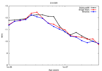
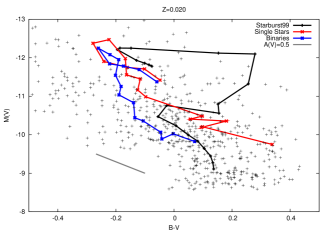
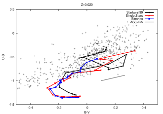
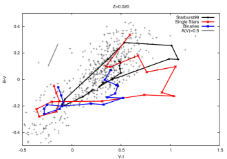
Before we compare our models to distant galaxies it is sensible to compare them to nearby unresolved stellar populations. Therefore we compare our models to a large set of observations of young massive star clusters compiled by Larsen & Richtler (1999). They observed a number of star clusters in nearby spiral galaxies with broad-band photometry. Since the host galaxies were spiral we assume the metallicity of the clusters is broadly solar and compare the observations to colours from our models for a cluster with a mass of . For comparison we have created a similar track from starburst99 with the same total stellar mass and initial mass distribution. This track was calculated using ‘Starburst99 for Windows’ (Leitherer & Chen, 2009) using the same IMF and total mass as for our models, the standard Geneva solar metallicity stellar evolution tracks, the Lejeune stellar atmosphere models and the remaining options at their default values. We plot the results in Figure 1. Our tracks are shorter than the starburst99 results as we terminate our simulations at 40 Myrs since we do not currently include stars with initial masses below which become important at times later than this.
From Figure 1 we see that the evolution of colours is broadly consistent between models and observations. However there are a number of important differences between the model tracks. These differences are primarily due to the different stellar models employed by starburst99 and the models presented here. Our model tracks tend to pass through regions of the diagram that contain more observed clusters although the observations have a large scatter, similar to the random error of the observations. In B-V the starburst99 models tend to have redder colours than our models at around 10 Myrs. However we see the greatest differences between the different model tracks in V-I. Our single star population tracks extend much further into the red than our binary models because binary models reduce the number of red supergiants and therefore reduce their contribution in the I band. However, the overproduction of red supergiants is a feature of all models containing only single stars (with the main difference being how those supergiants are characterised in the model population) and emphasises the need for binary population models.
Our binary models also tend to be bluer in B-V than our single star models, this is due to the increase in the number of main-sequence stars at late times due to secondaries accreting mass in binary interactions. We note that all the models plotted, those presented in this paper and similar models from starburst99, deviate from the locus of observed clusters in the B-V vs U-B colour plane at early times ( Myr), most likely due to variations in the metallicity of the clusters away from the Solar composition of our tracks. This deviation may also be due to relatively simple approximations for the strong nebular continuum contribution at these times. Models omitting this nebular contribution, while unphysical, can provide a better fit to the data in this region, suggesting that more detailed modelling of the nebular emission may be necessary.
There are a number of factors that we have not included in our model tracks presented here. For example we have not attempted to fit absorption from dust in the HII region Cloudy model. This is because the starburst99 model track does not include dust, only nebula continuum emission. In each of the panels we indicate the reddening direction for an of 0.5. We see that in some of the scatter of the observations could be explained by line of sight dust.
Given these caveats, we nonetheless find that binary populations have very different colours to a single star population at certain ages, and that the observational data at these points is often more consistent with the binary models with few sources showing V-I colours, for example, as extreme as those predicted for single star populations. To achieve this difference between the single and binary models, binaries with orbital separations between to must be included. Wider binaries do not interact so produce results little different from those from single stars. Tighter binaries tend to experience mergers and so, while evolving as binaries for some of their lives, they eventually become single stars.
3.2 Unresolved stellar populations from SDSS
Brinchmann, Kunth & Durret (2008) recently presented a study of a selection of SDSS galaxies showing evidence for ongoing massive star formation. They searched the SDSS DR6 archival spectra to identify those with Wolf-Rayet features in the optical. The two features used for identification are known as the blue and red Wolf-Rayet bumps at approximately 4700Å and 5800Å. These star-forming galaxies host massive stellar populations similar to those incorporated in our models, and hence provide a good experimental verification of the predictive power of our models. In order to construct an appropriate stellar population in our synthetic spectrum, we assume an instantaneous burst of star formation and consider its evolution with time222Note that this differs from our earlier work (Eldridge, Izzard & Tout, 2008), which considered continuous star formation.. We calculate the strength of Wolf-Rayet features both without and with a nebula emission model created with Cloudy as detailed in Section 2.4. Inclusion of nebular continuum emission leads to only a slight decrease in the maximum EW allowed by up to 10 percent.
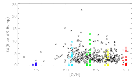
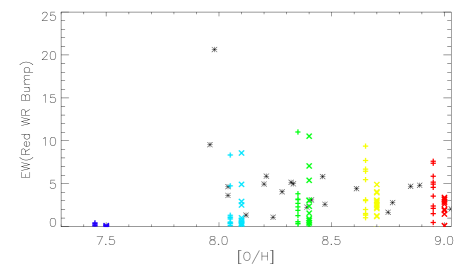
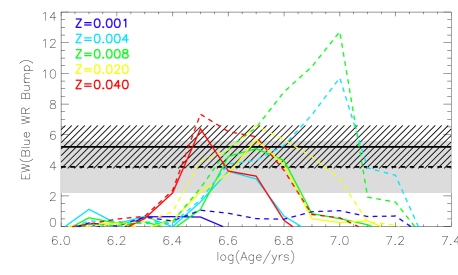
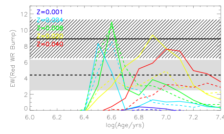
Here we calculate predicted values for the strength (equivalent width; EW) of Wolf Rayet features as defined by Brinchmann et al, removing the contribution of nebular lines to allow fair comparison with the data. As illustrated by Figures 2 and 3 in general our models reproduce the range of observed equivalent widths of both features with the exception of a few extreme cases.
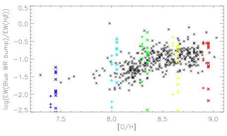
For a simple check of our nebula model, Figure 4 shows a comparison between the equivalent widths of the Blue WR bump to a nearby nebula emission line, H-. Comparing the ratio of these EWs will indicate whether we are estimating the strength of the nebula emission lines correctly relative to the stellar spectrum. We see that our model predictions of this ratio agree with the range of ratios from observed galaxies and previous estimates from the binary models of Van Bever & Vanbeveren (2003). Binary populations at metallicities below solar metallicity produce the highest ratio we discuss why this is below. We note our predicted ratios are a lower limit as the ratio we predict can be varied by changing the details of our Cloudy model, especially the covering factor. Decreasing this lets more ionising photons to escape and therefore decreases the nebula emission features such as the H- line luminosity without significantly affecting the blue WR bump EW which is determined by the stellar population. Thus the vertical spread has degeneracy between age and covering factor.
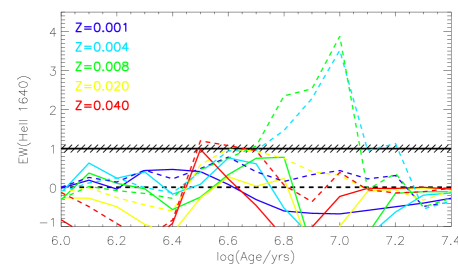
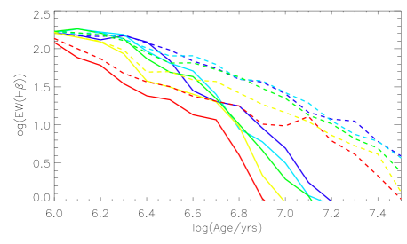
In Figure 5 we show the strength of the key Wolf-Rayet emission features in our model spectra as a function of the age of the stellar population and its metallicity. We see that the spread of values in Figures 2, 3 and 4 is due to a range of ages in the stellar population. Emission features peak at ages of a few million years for single stars and can be extended to much later times, up to 10 million years, by the inclusion of binaries. We note that similar diagrams with a nebula continuum component would reduce these observed EWs by a small amount. In Figure 6 we show how the strength of H- varies with age. We see that binary models exhibit H- to later ages. This is why at solar metallicity in Figure 4 at Solar metallicity single stars have a greater maximum ratio than binary stars, a smaller H- EW gives a larger ratio rather than great blue WR bump EW.
In Figure 5 there are large peaks in the strength of HeII and the blue WR bump at around 10 million years. These peaks are due to WNL stars formed from binary evolution. If these stars were in binaries they would be red supergiants. Their WNL phase has a long lifetime due to weak stellar winds at lower metallicities, so it takes longer for stellar winds and binary evolution to remove their hydrogen envelopes than at higher metallicity. Therefore their contribution to the composite spectrum is greater. Also as seen in Figure 6 the H- EW is small therefore artificially boosting the ratio of the two EW in Figure 4. If we only consider the ratio at ages less than years we do not achieve the highest ratios in Figure 4 and the ratio decreases with the same trend indicated by observations.
The reasons why such low metallicity systems with large ratios are not observed are related to the work of Charlot & Fall (2000) suggesting the gas in a massive cluster disperses by around 10 million years. With little gas surrounding the stars most ionising photons will escape producing little observation H- emission, effectively decreasing the covering factor. In the sample of SDSS galaxies we use only a few galaxies have H- EW less than 10Å. If the covering factor decreases with ages as suggested by the work of Charlot & Fall (2000), our predicted H- EW will drop below this value. Therefore it becomes less likely to observe the large ratios of blue WR bump EW to H- EW we predict in Figure 4.
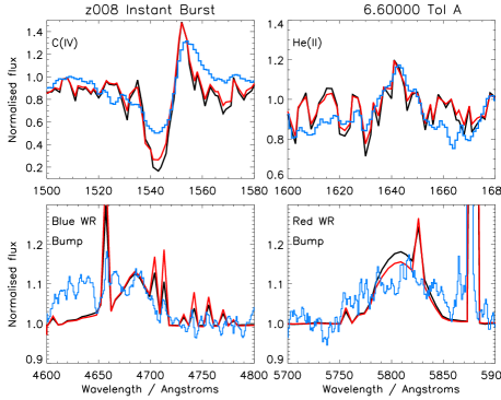
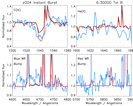
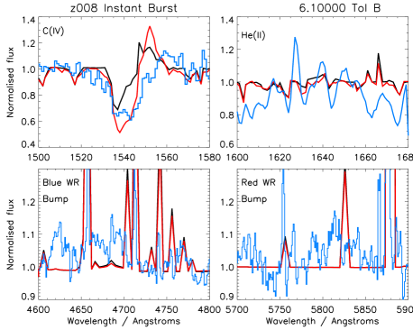
3.3 Comparison to the spectra of Tol A & B
A further comparison between our models and the integrated spectra of young stellar populations can be made using star forming regions with good spectral and photometric coverage. Sidoli, Smith & Crowther (2006) observed the massive stellar population in the giant HII region Tol89 in NGC5398. The published spectra of these regions span from the UV (useful for comparison to high redshift sources) to the optical (easily observed in more local galaxies). Sidoli, Smith & Crowther (2006) attempt to fit the observed Wolf-Rayet lines with a starburst99 model. They find that for the two knots of star formation, A & B, the ages are and Myrs respectively with an LMC-like metallicity, roughly two-fifths solar, preferred.
We attempt to fit the same spectra with our models. To do this we first measure the equivalent widths of the ultraviolet HeII 1640Å emission line and the Red and Blue Wolf-Rayet bumps in an identical manner on both the observed and model spectra. The HeII EW is calculated by normalising the spectra using the continuum points identified by Rix et al. (2004) and estimating the EW over the wavelength range 1635 to 1650Å. We calculate EWs for the WR bumps as in Section 3.2 but studying the spectrum to remove any (relatively narrow) nebula lines. The UV spectrum of Tol A is a stack of the spectra from 4 individual knots of star formation. We find one of these knots, A4 as identified by Sidoli, Smith & Crowther (2006) has a very narrow nebula emission of HeII at 1640Å. This dominates the EW of the A4 knot and has an equivalent width of 0.2Å in the Tol A stack. Nebula HeII emission indicates a very hard ionising radiation field in this cluster. It has been suggested such lines indicate the presence of population III stars (Schaerer, 2003). However in this case the hard ionising field is more likely to come from some other source given the relatively high metallicity and zero redshift. For example that knot is old enough that there could be an accreting black hole or neutron star present producing harder radiation. We have not yet attempted to include such emission in our models yet. Therefore we have calculated the EW of the HeII line of Tol A ignoring the A4 knot.
We plot our model line strengths against age in Figure 5 compared to the observed EW of features in the Tol A & B regions. We find that single star and binary models are both able to reproduce the observed EW in these features simultaneously at around years. We also show how show how the H- EW varies with age in Figure 6. While we find that the EW broadly agrees with those observed for Tol A & B we do not use them to derive the ages of the stellar population.
The best fit metallicity is an LMC-like metallicity of . The age of Tol A is constrained to be from and years. At ages outside this range the stellar features are too weak to agree with the observed values, or for the binary models, too strong. For Tol B the age is constrained to be less than years.
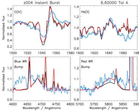
To verify the best fit ages and metallicities we show a more detailed comparison between these models and the observed spectra for Tol A and B in Figures 7 and 8 respectively, considering the three key WR diagnostic features and also the ultraviolet CIV absorption/emission feature at 1550Å, which is sensitive to the presence of massive stars and in particular winds driven from O-stars. For Tol A, we find reasonable visual fits between and years at both SMC () and LMC metallicities. The CIV line requires younger ages for the system than the WR features provide. For Tol B we find any model with negligible HeII emission provides a reasonable fit to the data. However models with ages of years and older tend to overpredict the CIV emission line relative the observed spectrum. Also for the blue and red bumps there are no distinctive broad emission lines and the spectrum is dominated by narrow emission lines. This again suggests a young population.
Our derived ages, both from matching the spectra by eye and from the line equivalent widths, are 4 Myrs for Tol A and Myrs for Tol B. These agree with the ages of Sidoli, Smith & Crowther (2006). However our ages are on the young side of the ages they derived.
By eye the model agreement is good, especially in light of the general models employed, which are not fine-tuned to any great degree. The line profiles and strengths of ultraviolet spectral features are generally less well fit than the optical features. There are several ways in which our models might be fine tuned to fit the observational data in this case. Firstly, it may be possible to refine our model for nebular continuum contribution to the integrated spectrum. At present, we consider a basic model as discussed above and parameters could be adjusted to gain a better fit for this star-forming region. Secondly, it may be possible to include the effects of material external to the system in addition to gas and dust local to the star-forming region which is modelled using Cloudy. Thirdly, we only use a sparse grid of O-star models rather than a dense grid of atmospheres and it may be possible to improve upon this in future (Rix et al., 2004). Fourthly, we have assumed an instantaneous burst. A better fit might be achieved by allowing multiple star formation episodes with slightly different ages. Fifthly we have not considered the effects of stellar rotation on the evolution or the spectra. This will have two effects on our results. It would extend the main-sequence life-time and would also rotationally broaden the CIV line further, particularly if the stars rotate at velocities above . This would potentially improve the fit between models and observed data. We speculate that study of the CIV profile could potentially give a way to evaluate the importance of rotation versus binarity in stellar populations. Finally, some WNL stars have CIV in emission. We have not included any such CIV emission in the WNL stars that are not represented by the Potsdam model atmospheres. Including an empirical correction for such emission in these models may broaden the emission component of the CIV line and simultaneously decrease the absorption component. However we do not choose to introduce arbitrary line emission here.
4 Discussion and Conclusions
In this paper we set out to describe the construction of model stellar populations incorporating massive stars and massive stellar binaries, and then the synthesis of spectra for this population. We have compared our model spectra to observations of comparable unresolved stellar populations and found agreement is fair over a large range of wavelengths, from the UV to the near infra-red.
In general our population synthesis including binary models predict that such systems have less emission at long wavelengths around the I band. This is because binary interactions remove the hydrogen envelope of some red supergiants to form Wolf-Rayet stars. These WR stars then lead to more blue colours in B-V and V-I broad-band colours and a larger UV flux. The latter increases the timespan over which nebula emission is important to the evolution of stellar populations from 6 Myrs to 20 Myrs. Another binary effect is that it is more likely that strong WR emission lines are observed since binary interactions tend to spread WR emission features over a longer timespan. For single stars the WR stars all exist over a short timespan so WR features are only present for a short period of time. This suggests that ages derived from Wolf-Rayet features to date may have been systematically underestimated.
It may be somewhat surprising that by including binary evolution we find no great difference from predictions from starburst99, a code based on single-star evolution alone. However the stellar evolution models used in the starburst99 model present in Section 3.1 are nearly two decades old (Schaller et al., 1992). The important difference between these models and those used here is that the mass-loss rates have substantially decreased for OB-stars and WR stars. Therefore with incorrect single-star mass-loss rates the older models reproduce the observed stellar population. Our model binary population therefore should broadly agree with this older code, but now we model the same magnitude of mass-loss as a combination of lower single-star mass-loss rates enhanced for some stars by binary interactions which is a physically reasonable model.
We demonstrate that our code produces a good fit to the observational data of local stellar populations in which massive stars are important. However, further refinements are possible and additional verification data on local star-forming regions would be welcome. Nonetheless, the stellar models and synthesis code presented here may now be used as a tool to study stellar populations in a range of different observational domains and to derive their physical parameters, as demonstrated by their application to extragalactic star-forming regions Tol A and B.
Acknowledgements
The authors would like to thank the referee Jarle Brinchmann for his very helpful and constructive comments. The authors also thank Malcolm Bremer, Max Pettini, Paul Crowther, Stephen Smartt, Nate Bastian and Norbert Langer for useful discussions. ERS acknowledges postdoctoral research support from the UK Science and Technology Facilities Council (STFC). JJE began this work when he was supported by the award “Understanding the lives of massive stars from birth to supernovae” made under the European Heads of Research Councils and European Science Foundation EURYI Awards scheme which is supported by funds from the Participating Organisations of EURYI and the EC Sixth Framework Programme. JJE also acknowledges support from the UK Science and Technology Facilities Council (STFC) under the rolling theory grant for the Institute of Astronomy.
References
- Belkus et al. (2003) Belkus H., Van Bever J., Vanbeveren D., van Rensbergen W., 2003, A&A, 400, 429
- Brandt & Podsiadlowski (1995) Brandt N., Podsiadlowski P., 1995, MNRAS, 274, 461B
- Brinchmann, Pettini & Charlot (2008) Brinchmann J., Pettini M., Charlot S., 2008, MNRAS, 385, 769B
- Brinchmann, Kunth & Durret (2008) Brinchmann J., Kunth D., Durret F., 2008, A&A, 485, 657B
- Cantiello et al. (2007) Cantiello M., Yoon S.-C., Langer N., Livio M., 2007, A&A, 465L, 29C
- Charlot & Fall (2000) Charlot S., Fall S.M., 2000, ApJ, 539, 718
- Conroy, Gunn & White (2008) Conroy C., Gunn J.E., White M., 2009, ApJ, 699, 486
- Crowther & Hadfield (2006) Crowther P. A., Hadfield L. J., 2006, A&A, 449, 711
- de Mink et al. (2009) de Mink S. E., Cantiello M., Langer N., Pols O. R., Brott I., Yoon S.-Ch., 2009, A&A, 497 243
- Dionne & Robert (2006) Dionne D., Robert C., 2006, ApJ, 641, 252
- Eggleton (1971) Eggleton P.P., 1971, MNRAS, 151, 351
- Eldridge et al. (2006) Eldridge J.J., Genet F., Daigne F., Mochkovitch R., 2006, MNRAS, 367, 186E
- Eldridge & Vink (2006) Eldridge J.J., Vink J.S., 2006, A&A, 452, 295
- Eldridge, Mattila & Smartt (2007) Eldridge J. J., Mattila S., Smartt S.J., 2007, MNRAS, 376L, 52E
- Eldridge, Izzard & Tout (2008) Eldridge J.J., Izzard R.G., Tout C.A., 2008, MNRAS, 384, 1109
- Ferland et al. (1998) Ferland G.J., Korista K.T., Verner D.A., Ferguson J.W., Kingdon J.B., Verner E.M., 1998, PASP, 110, 761
- Hamann, Gräfener & Liermann (2006) Hamann W.-R., Gräfener G., Liermann A., 2006, A&A, 457, 1015H
- Han et al. (2007) Han Z., Podsiadlowski Ph., Lynas-Gray A.E., 2007, MNRAS, 380, 1098
- Hobbs et al. (2005) Hobbs G., Lorimer D.R., Lyne A.G., Kramer M., 2005, MNRAS, 360, 974H
- Hurley, Pols & Tout (2000) Hurley J.R., Pols C.A., Tout O.R., 2000, MNRAS, 315, 543H
- Hurley, Tout & Pols (2002) Hurley J.R., Tout C.A., Pols O.R. 2002, MNRAS, 329, 897
- Kroupa, Tout & Gilmore (1993) Kroupa P., Tout C.A., Gilmore G., 1993, MNRAS, 262, 545
- Larsen & Richtler (1999) Larsen S.S., Richtler T., 1999, A&A, 345, 59
- Leitherer et al. (1999) Leitherer C., et al., 1999, ApJS, 123, 3
- Leitherer & Chen (2009) Leitherer C., Chen J., 2009, NewA, 14, 356L
- Maeder & Meynet (2005) Meynet G., Maeder A., 2005, A&A, 429, 581
- Molla et al. (2009) Molla M., Garcia-Vargas M.L., Bressan A., 2009, MNRAS in press
- Rix et al. (2004) Rix S. A., Pettini M., Leitherer C., Bresolin F., Kudritzki R.-P., Steidel C. C., 2004,
- Schaerer & Vacca (1998) Schaerer D., Vacca W.D., 1998, ApJ, 497, 618
- Schaerer (2002) Schaerer D., 2002, A&A, 382, 28
- Schaller et al. (1992) Schaller G., Schaerer D., Meynet G., Maeder A., 1992, A&AS, 96, 269S
- Schaerer (2003) Schaerer D., 2003, A&A, 397, 527
- Sidoli, Smith & Crowther (2006) Sidoli F., Smith L.J., Crowther P.A., 2006, MNRAS, 370, 799S
- Smith, Norris & Crowther (2002) Smith L.J., Norris R.P.F., Crowther P.A., 2002, MNRAS, 337, 1309S
- Stancliffe & Eldridge (2009) Stancliffe R. J., Eldridge J. J., 2009, MNRAS, 396, 1699
- Van Bever & Vanbeveren (1998) van Bever J., Vanbeveren D., 1998, A&A, 334, 21V
- Van Bever & Vanbeveren (2003) van Bever J., Vanbeveren D., 2003, A&A, 400, 63V
- Vázquez et al. (2007) V zquez G.A., Leitherer C., Schaerer D., Meynet G., Maeder A., 2007, ApJ, 663, 995V
- Westera et al. (2002) Westera P., Lejeune T., Buser R., Cuisinier F., Bruzual G., 2002, A&A, 381, 524W
- Zackrisson, Bergvall & Leitet (2008) Zackrisson E., Bergvall N., Leitet E., 2008, ApJ, 676L, 9