Distinct scalings for mean first-passage time of random walks on scale-free networks with the same degree sequence

Abstract

In general, the power-law degree distribution has profound influence on various dynamical processes defined on scale-free networks. In this paper, we will show that power-law degree distribution alone does not suffice to characterize the behavior of trapping problem on scale-free networks, which is an integral major theme of interest for random walks in the presence of an immobile perfect absorber. In order to achieve this goal, we study random walks on a family of one-parameter (denoted by $q$) scale-free networks with identical degree sequence for the full range of parameter $q$, in which a trap is located at a fixed site. We obtain analytically or numerically the mean first-passage time (MFPT) for the trapping issue. In the limit of large network order (number of nodes), for the whole class of networks, the MFPT increases asymptotically as a power-law function of network order with the exponent obviously different for different parameter $q$, which suggests that power-law degree distribution itself is not sufficient to characterize the scaling behavior of MFPT for random walks, at least trapping problem, performed on scale-free networks.

I Introduction

As a fundamental stochastic process, random walks have received considerable attention from the scientific society, since they found a wide range of distinct applications in various theoretical and applied fields, such as physics, chemistry, biology, computer science, among others Sp1964 ; We1994 ; Hu1996 . Among a plethora of interesting issues of random walks, trapping is an integral major one, which plays an important role in an increasing number of disciplines. The so-called trapping issue that was first introduced in Mo69 , is a random-walk problem, where a trap is positioned at a fixed location, absorbing all particles that visit it. The highly desirable quantity closed related to the trapping issue is the first-passage time (FPT), also called trapping time (TT). The FPT for a given site (node, vertex) is the time spent by the walker starting from the site to hit the trap node for the first time. The average of first-passage times over all nodes is referred to as the mean first-passage time (MFPT), or mean trapping time (MTT), which is frequently used to measure the efficiency of the trapping problem.

One of the most important questions in the research of trapping is determining its efficiency, namely, showing the dependence relation of MFPT on the size of the system where the random walks are performed. Previous studies have provided the answers to the corresponding problems in some particular graphs with simple structure, such as regular lattices Mo69 , Sierpinski fractals KaBa02PRE ; KaBa02IJBC , T-fractal Ag08 , and so forth. However, recent empirical studies AlBa02 ; DoMe02 ; Ne03 uncovered that many (perhaps most) real networks are scale-free characterized by a power-law degree distribution BaAl99 , which cannot be described by above simple graphs. Thus, it appears quite natural and important to explore the trapping issue on scale-free networks. In recent work ZhQiZhXiGu09 ; ZhGuXiQiZh09 ; ZhZhXiChLiGu09 , we have shown that scale-free property may substantially improve the efficiency of the trapping problem: the MFPT behaves linearly or sublinearly with the order (number of nodes) of the scale-free networks, which is in sharp contrast to the superlinear scaling obtained for above-mentioned simple graphs Mo69 ; KaBa02PRE ; KaBa02IJBC ; Ag08 . It was speculated that the high efficiency of trapping on scale-free networks is attributed to their power-law property. Although scale-free feature can strongly affect the various dynamics occurring on networks, it was shown that the scale-free structure itself does not suffice to characterize some dynamical processes on networks, e.g., synchronization AtBiJo06 ; HaSwSc06 , disease spreading EgKl02 ; ZhZhZoCh08 , and the like. Thus far, it is still unknown whether the power-law degree distribution is sufficient to characterize the behavior of trapping problem on scale-free networks.

In this paper, we study the trapping problem on the a class of scale-free networks with the same degree sequence, which are dominated by a tunable parameter $q$ ZhZhZoChGu09 . We determine separately the explicit formulas of the mean first-passage time for the two limiting cases of $q=1$ and $q=0$. We show that in both cases the MFPT increases as a power-law function of the network order, with the exponent less than 1 for $q=1$ and equal to 1 for $q=0$. We also study numerically the MFPT for the case of $0<q<1$, finding that it is also a power-law function of network order with the exponent $\theta(q)$ depending on parameter $q$. We demonstrate that in the full range of $0\leq q\leq 1$, $\theta(q)$ is a decreasing function of $q$, which belongs to the interval $\left[\frac{\ln 3}{\ln 4},1\right]$. Our findings indicate that the power-law degree distribution by itself is not sufficient to characterize the trapping process taking place on scale-free networks.

II The scale-free networks with identical degree sequence

Figure 1: Iterative method of the network construction. Each edge is replaced by either of the connected clusters on the right-hand side of arrows with a certain probability, where black squares represent new nodes.

The networks in question are built iteratively ZhZhZoChGu09 , see Fig. 1. We represent by $H_{n}$ ($n\geq 0$) the networks after $n$ iterations (the number of iterations is also called generation hereafter). Then the networks are constructed as follows. For $n=0$, the initial network $H_{0}$ consists of two nodes connected to each other by an edge (a link). For $n\geq 1$, $H_{n}$ is obtained from $H_{n-1}$. That is to say, to obtain $H_{n}$, one can replace each link existing in $H_{n-1}$ either by a connected cluster of links on the top right of Fig. 1 with probability $q$, or by the connected cluster on the bottom right with complementary probability $1-q$. Repeat the growth process $n$ times, with the graphs obtained in the limit $n\to\infty$. In Figs. 2 and 3, we present the growing processes of two special networks corresponding to $q=0$ and $q=1$, respectively.

Figure 2: (Color online) Illustration of the first several iterations of the network for a particular case $q=1$.

Let $L(n)$ be the number of nodes created at generation $n$, and $E_{n}$ the total number of all edges present at generation $n$. By construction, we have $E_{n}=4\,E_{n-1}$. Considering the initial condition $E_{0}=2$, it leads to $E_{n}=4^{n}$. Since each existing edge at a given generation will create two new nodes in at the next generation, then, at each generation $n_{i}$ ($n_{i}\geq 1$) the number of newly introduced nodes is $L(n_{i})=2E_{n_{i}-1}=2\times 4^{n_{i}-1}$. Thus, at generation $n$ the network order is

$$V_{n}=\sum_{n_{i}=0}^{n}L(n_{i})=\frac{2}{3}(4^{n}+2)\,.$$ (1)

Let $k_{i}(n)$ be the degree of a node $i$ at generation $n$, which was created at generation $n_{i}$ ($n_{i}\geq 0$). Then,

$$k_{i}(n)=2^{n-n_{i}+1}\,.$$ (2)

From Eq. (2), it is obvious that after each new iteration the degree of a node doubles, i.e.,

$$k_{i}(n)=2\,k_{i}(n-1)\,.$$ (3)

Figure 3: Sketch of the iteration process of the network for the limiting case of $q=0$.

The networks considered exhibit some interesting topological properties. Their nodes have same degree sequence (thus the same degree distribution), independent of the value of parameter $q$. Concretely, the networks have a power-law degree distribution with the exponent $\gamma=3$ ZhZhZoChGu09 . On the other hand, since there is no triangle in the whole class of the networks, the clustering coefficient is zero. Although the degree distribution and clustering coefficient do not depend on the parameter $q$, other structural characteristics are closely related to $q$. For example, for $q=1$, the network is reduced to the (2, 2)-flower introduced in RoHaAv07 . In this case, it is a small world, its average path length (APL), defined as the mean of shortest distances between all pairs of nodes, grows logarithmically with the network order ZhZhZoChGu09 ; at the same time, it is a non-fractal network SoHaMa05 ; SoHaMa06 . While for $q=0$, it is exactly the hierarchical lattice that was proposed by Berker and Ostlund BeOs79 and was extensively studied by many authors KaGr81 ; GrKa82 ; HiBe06 ; ZhZhZo07 ; RoAv07 ; ArBe09 . For this case, the network is not small-world with the APL increasing as a square power of the network order HiBe06 ; ZhZhZo07 ; moreover, it is fractal with the fractal dimension $d_{B}=2$. When $q$ increases from 0 to 1, the networks undergo a transition from fractal to non-fractal scalings, and exhibit a crossover from ‘large’ to small worlds at the same time ZhZhZoChGu09 ; these similar phenomena are also observed in a family of treelike networks ZhZhChGu08 .

The peculiar topological features make the networks unique within the category of scale-free networks, since these particular structures strongly affect the dynamical processes defined on the networks. For instance, different thresholds of bond percolation were recently observed in the networks, which implies that power-law degree distribution alone does not suffice to characterize the percolation threshold on scale-free networks under bond percolation ZhZhZoChGu09 ; RoAv07 . In what follows, we will study random walks with a single immobile trap on the networks. We will show that the degree distribution is not sufficient to determine the scalings for MFPT of trapping process occurring on the networks under consideration.

III Random walks with a fixed trap

In this section, we study the so-called simple discrete-time random walks of a particle on network $H_{n}$. At each time step, the particle (walker) jumps from its current location to one of its neighbors with equal probability. In particular, we focus on the trapping problem, i.e., a special issue for random walks with a trap positioned at a given node. To this end, we first we distinguish different nodes in $H_{n}$, by labeling them in the following way. The two nodes in $H_{0}$ have labels 1 and 2. For each new generation, we only label the new nodes created at this generation, while we keep the labels of all pre-existing nodes unchanged. In other words, we label sequentially new nodes as $M+1,M+2,\ldots,M+\Delta M$, where $M$ is the number of the old nodes and $\Delta M$ the number of newly-created nodes. In this way, every node is labeled by a unique integer, at generation $n$ all nodes are labeled from 1 to $V_{n}=\frac{2}{3}(4^{n}+2)$. Figures 4 and 5 show how the nodes are labeled for two special cases of $q=1$ and $q=0$.

Figure 4: labels of all nodes of ${H}_{3}$ in the case of $q=1$.

Figure 5: labels of all nodes of ${H}_{3}$ for the particular case of $q=0$.

We place the trap at node 1, denoted by $i_{T}$. At each time step, the particle, starting from any node except the trap $i_{T}$, moves uniformly to any of its nearest neighbors. It should be mentioned that, due to the symmetry, the trap can be also situated at nodes 2, 3, or 4, which has not any effect on MFPT. The special selection we made for the trap allows to address the issue conveniently. Particularly, this makes it possible to analytically compute the MFPT for the two deterministic networks corresponding to $q=1$ and $q=0$ (details will be discussed below), because of their special structures and the convenience of identifying the trap $i_{T}$ since the first generation.

As mentioned above, one of the most important quantity characterizing such a trapping problem is the FPT defined as the expected time a walker takes, starting from a source node, to first reach the trap node. The significance firstly originates from the fact that the first encounter properties are relevant to those in a plethora of real situations CoBeTeVoKl07 , including transport, disease spreading, target search, and so on. On the other hand, many other quantities can be expressed in terms of FPTs, and more information about the dynamics of random walks can be extracted from the analysis of FPTs Re01 . Finally, the average of first-passage times, i.e., mean first-passage time (MFPT), measures the efficiency of the trapping process: the smaller the MFPT, the higher the efficiency, and vice versa. In the following, we will determine the exact solutions to MFPT for some limiting cases, as well as the dependence relation of MFPT on the network order.

Let $T_{i}^{(n)}$ be the FPT for a walker initially placed at node $i$ to first reach the trap $i_{T}$ in $H_{n}$. This quantity can be expressed in terms of mean residence time (MRT) BaKl98 ; ZhZhXiChLiGu09 , which is defined to be the mean time that a random walker spends at a given node prior to being absorbed by the trap. Actually, the MRT is the mean number of visitations of a given node by the walker before trapping occurs.

It is known that the trapping problem studied can be described by a Markov chain KeSn76 , whose fundamental matrix is the inverse of matrix $\mathbf{B}_{n}$ that is a variant of the normalized Laplacian matrix Ch97 $\mathbf{L}_{n}$ for $H_{n}$, and can be obtained from $\mathbf{L}_{n}$ with all entries in the first row and column (corresponding to the trap node) setting to zeros. The entry $(b_{n}^{-1})_{ij}$ of the fundamental matrix $(\mathbf{B}_{n})^{-1}$ expresses the mean number of visitations of node $j$ by the particle, starting from node $i$, before it is eventually trapped. Thus, we have

$$T_{i}^{(n)}=\sum_{j=2}^{V_{n}}(b_{n}^{-1})_{ij}\,.$$ (4)

Then, the mean first-passage time, $\langle T\rangle_{n}$, which is the average of $T_{i}^{(n)}$ over all initial nodes distributed uniformly over nodes in $H_{n}$ other than the trap, is given by

$$\langle T\rangle_{n}=\frac{1}{V_{n}-1}\sum_{i=2}^{V_{n}}T_{i}^{(n)}=\frac{1}{V_{n}-1}\sum_{i=2}^{V_{n}}\sum_{j=2}^{V_{n}}(b_{n}^{-1})_{ij}\,.$$ (5)

Equation (5) shows that the problem of determining $\langle T\rangle_{n}$ is reduced to computing the sum of all elements of the fundamental matrix $(\mathbf{B}_{n})^{-1}$. Although the expression of Eq. (5) seems compact, the complexity of inverting $\mathbf{L}_{n}$ is O($V_{n}^{3}$). Since the network order increases exponentially with $n$, Eq. (5) becomes intractable for large $n$. Thus, restricted by time and computer memory, one can obtain $\langle T\rangle_{n}$ through direct calculation from Eq. (5) only for the first iterations. It would be satisfactory if good alternative computation methods could be proposed to get around this problem. What is encouraging is that the particular construction of the networks and the special choice of the trap location allow to calculate analytically MFPT to obtain a closed-form formula, at least for the two special cases of $q=1$ and $q=0$. The computation details will be provided in the following text.

III.1 Case of $q=1$

We first establish the scaling relation governing the evolution for $T_{i}^{(n)}$ with generation $n$. In Table 1, we list the numerical values of $T_{i}^{(n)}$ for some nodes up to $n=6$. From the numerical values, we can observe that for a given node $i$, the relation $T_{i}^{(n+1)}=3\,T_{i}^{(n)}$ holds. That is to say, upon growth of the network from generation $n$ to generation $n+1$, the trapping time to first arrive at the trap increases by a factor $3$. This is a basic characteristic of random walks on $H_{n}$ when $q=1$, which can be established from the arguments below HaBe87 ; KaRe89 ; Bobe05 .

Table 1: Numerical results of the trapping time $T_{i}^{(n)}$ for a random walker starting from node $i$ on the network $H_{n}$ for various $n$ in the case of $q=1$. All the values are obtained through the direct calculation from Eq. (4).

$n\backslash i$	2,3	4	5,6	7,8	9,10	11,12	13,14	15,16	17,18	19,20	21,22	23,24	25,26	27,28	29-32	33-36	37-40	41-44
1	$3$	$4$
2	$9$	$12$	$5$	$8$	$12$	$13$
3	$27$	$36$	$15$	$24$	$36$	$39$	$7$	$12$	$20$	$23$	$27$	$28$	$11$	$20$	$32$	$35$	$39$	$40$
4	$81$	$108$	$45$	$72$	$108$	$117$	$21$	$36$	$60$	$69$	$81$	$84$	$33$	$60$	$96$	$105$	$117$	$120$
5	$243$	$324$	$135$	$216$	$324$	$351$	$63$	$108$	$180$	$207$	$243$	$252$	$99$	$180$	$288$	$315$	$351$	$360$
6	$729$	$972$	$405$	$648$	$972$	$1053$	$189$	$324$	$540$	$621$	$729$	$756$	$297$	$540$	$864$	$945$	$1053$	$1080$

Consider an arbitrary node $i$ in $H_{n}$ of the $q=1$ case, after $n$ generation evolution. From Eq. (3), we know that upon growth of the network to generation $n+1$, the degree, $k_{i}$, of node $i$ doubles, namely, it increases from $k_{i}$ to $2\,k_{i}$. Among these $2\,k_{i}$ neighbors, one half are old neighbors, while the other half are new nodes created at generation $n+1$, each of which has two connections, attached to node $i$ and another simultaneously emerging new node. We now examine the standard random walk in $H_{n+1}$: Let $X$ be the FPT for a particle going from node $i$ to any of its $k_{i}$ old neighbors; let $Y$ be the FPT for going from any of the $k_{i}$ new neighbors of $i$ to one of the $k_{i}$ old neighbors; and let $Z$ represent the FPT for starting from any of new neighbors (added to the network at generation $n+1$) of an old neighbor of $i$ to this old neighbor. Then we can establish the following backward equations:

$$\left\{\begin{array}[]{ccc}X&=&\frac{1}{2}+\frac{1}{2}(1+Y)\,,\\ Y&=&\frac{1}{2}(1+X)+\frac{1}{2}(1+Z)\,,\\ Z&=&\frac{1}{2}+\frac{1}{2}(1+Y)\,.\end{array}\right.$$ (9)

Equation (9) has a solution $X=3$. Thus, upon the growth of the network from generation $n$ to generation $n+1$, the first-passage time from any node $i$ to any node $j$ (both $i$ and $j$ belong to $H_{n}$) increases by a factor of 3. That is to say, $T_{i}^{(n+1)}=3\,T_{i}^{(n)}$, which will be useful for the derivation of the exact formula for the MFPT below.

After obtaining the scaling of first-passage time for old nodes, we now derive the analytical rigorous expression for the MFPT $\langle T\rangle_{n}$. Before proceeding further, we first introduce the notations that will be used in the rest of this section. Let $\Delta_{n}$ denote the set of nodes in $H_{n}$, and let $\overline{\Delta}_{n}$ stand for the set of those nodes entering the network at generation $n$. For the convenience of computation, we define the following quantities for $1\leq m\leq n$:

$$T_{m,{\rm tot}}^{(n)}=\sum_{i\in\Delta_{m}}T_{i}^{(n)},$$ (10)

and

$$\overline{T}_{m,{\rm tot}}^{(n)}=\sum_{i\in\overline{\Delta}_{m}}T_{i}^{(n)}.$$ (11)

By definition, it follows that $\Delta_{n}=\overline{\Delta}_{n}\cup\Delta_{n-1}$. Thus, we have

$$T_{n,{\rm tot}}^{(n)}=T_{n-1,{\rm tot}}^{(n)}+\overline{T}_{n,{\rm tot}}^{(n)}=3\,T_{n-1,{\rm tot}}^{(n-1)}+\overline{T}_{n,{\rm tot}}^{(n)}\,,$$ (12)

where the relation of $T_{i}^{(n+1)}=3\,T_{i}^{(n)}$ has been made use of. Hence, in order to determine $\overline{T}_{n,{\rm tot}}^{(n)}$, we should first find the quantity $\overline{T}_{n,{\rm tot}}^{(n)}$ that can be obtained as follows.

Figure 6: (Color online) Illustration showing the relation of the mean transmit times for two new nodes and two old nodes connected by an edge generating the new nodes.

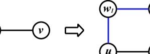
By construction, at a given generation, for each edge connecting two nodes $u$ and $v$ (see Fig. 6), it will generate two new nodes (say $w_{1}$ and $w_{2}$) in the next generation, and the mean transmit times for the two new nodes obey the following relations:

$$\left\{\begin{array}[]{ccc}T(w_{1})&=&\frac{1}{2}(1+T(w_{2}))+\frac{1}{2}\left(1+T(u)\right)\,,\\ T(w_{2})&=&\frac{1}{2}(1+T(w_{1}))+\frac{1}{2}\left(1+T(v)\right)\,.\end{array}\right.$$ (15)

Hence, we have

$$T(w_{1})+T(w_{2})=4+T(u)+T(v)\,.$$ (16)

Summing Eq. (16) over all the $E_{n}$ old edges pre-existing at the generation $n$, we obtain

$$\overline{T}_{n+1,{\rm tot}}^{(n+1)} = 4\,E_{n}+\sum_{i\in\Delta_{n}}\left(k_{i}(n)\times T_{i}^{(n)}\right)$$ (17)

$$= 4^{n+1}+2\,\overline{T}_{n,{\rm tot}}^{(n+1)}+2^{2}\,\overline{T}_{n-1,{\rm tot}}^{(n+1)}+\ldots$$

$$+2^{n}\,\overline{T}_{1,{\rm tot}}^{(n+1)}+2^{n}\,\overline{T}_{0,{\rm tot}}^{(n+1)}\,.$$

For example, in $H_{2}$ (see Fig. 4), $\overline{T}_{2,{\rm tot}}^{(2)}$ can be expressed as

$$\overline{T}_{2,{\rm tot}}^{(2)} = \left(T_{5}^{(2)}+T_{6}^{(2)}\right)+\left(T_{7}^{(2)}+T_{8}^{(2)}\right)$$ (18)

$${}+\left(T_{9}^{(2)}+T_{10}^{(2)}\right)+\left(T_{11}^{(2)}+T_{12}^{(2)}\right)$$

$$= \left(4+T_{1}^{(2)}+T_{2}^{(2)}\right)+\left(4+T_{2}^{(2)}+T_{3}^{(2)}\right)$$

$$+\left(4+T_{3}^{(2)}+T_{4}^{(2)}\right)+\left(4+T_{4}^{(2)}+T_{1}^{(2)}\right)$$

$$= 4\,E_{1}+2\left(T_{1}^{(2)}+T_{2}^{(2)}+T_{3}^{(2)}+T_{4}^{(2)}\right)$$

$$= 16+2\,\overline{T}_{1,{\rm tot}}^{(2)}+2\,\overline{T}_{0,{\rm tot}}^{(2)}\,.$$

Again, for instance, in $H_{3}$ (see Fig. 4), $\overline{T}_{3,{\rm tot}}^{(3)}$ can be written as

$$\overline{T}_{3,{\rm tot}}^{(3)}=64+2\,\overline{T}_{2,{\rm tot}}^{(3)}+4\,\overline{T}_{1,{\rm tot}}^{(3)}+4\,\overline{T}_{0,{\rm tot}}^{(3)}\,.$$ (19)

Now, we can determine $\overline{T}_{n,{\rm tot}}^{(n)}$ through a recurrence relation, which can be obtained easily. From Eq. (17), it is not difficult to write out $\overline{T}_{n+2,{\rm tot}}^{(n+2)}$ as

$$\overline{T}_{n+2,{\rm tot}}^{(n+2)}=4^{n+2} + 2\,\overline{T}_{n+1,{\rm tot}}^{(n+2)}+2^{2}\,\overline{T}_{n,{\rm tot}}^{(n+2)}+\ldots$$ (20)

$$+ 2^{n+1}\,\overline{T}_{1,{\rm tot}}^{(n+2)}+2^{n+1}\,\overline{T}_{0,{\rm tot}}^{(n+2)}\,.$$

Equation (20) minus Eq. (17) times 6 and applying the relation of $T_{i}^{(n+2)}=3\,T_{i}^{(n+1)}$, one gets the following recurrence relation

$$\overline{T}_{n+2,{\rm tot}}^{(n+2)}=12\,\overline{T}_{n+1,{\rm tot}}^{(n+1)}-2\times 4^{n+1}\,.$$ (21)

Using $\overline{T}_{1,{\rm tot}}^{(1)}=7$, Eq. (21) is solved inductively

$$\overline{T}_{n,{\rm tot}}^{(n)}=4^{n-1}+6\times 12^{n-1}\,.$$ (22)

Inserting Eq. (22) into Eq. (12) leads to

$$T_{n,{\rm tot}}^{(n)}=3\,T_{n-1,{\rm tot}}^{(n-1)}+4^{n-1}+6\times 12^{n-1}\,.$$ (23)

Considering the initial condition $T_{1,{\rm tot}}^{(1)}=10$, Eq. (23) is resolved by induction to obtain

$$T_{n,{\rm tot}}^{(n)}=\frac{2}{3}\times 12^{n}+4^{n}-2\times 3^{n-1}\,.$$ (24)

Substituting Eq. (24) into Eq. (5), we obtain the closed-form expression for the MFPT for the trapping problem on $H_{n}$ of the $q=1$ case as follows:

$$\langle T\rangle_{n}=\frac{1}{V_{n}-1}T_{n,{\rm tot}}^{(n)}=\frac{1}{2\times 4^{n}+1}(2\times 12^{n}+3\times 4^{n}-2\times 3^{n})\,.$$ (25)

Below we will show how to express $\langle T\rangle_{n}$ in terms of network order $V_{n}$, with the aim of obtaining the relation between these two quantities. Recalling Eq. (1), we have $4^{n}=\frac{3}{2}V_{n}-2$ and $n=\log_{4}\big{(}\frac{3}{2}V_{n}-2\big{)}$. Thus, Eq. (25) can be rewritten as

$$\langle T\rangle_{n}=\frac{V_{n}-2}{V_{n}-1}\left(\frac{3}{2}V_{n}-2\right)^{\frac{\ln 3}{\ln 4}}+\frac{3V_{n}-4}{2(V_{n}-1)}.$$ (26)

For large network, i.e., $V_{n}\rightarrow\infty$,

$$\langle T\rangle_{n}\sim(V_{n})^{\ln 3/\ln 4}\,,$$ (27)

with the exponent less than 1. Thus, in large network the MFPT grows sublinearly with network order.

Table 2: The trapping time $T_{i}^{(n)}$ for a random walker starting from node $i$ on the network $H_{n}$ for various $n$ in the case of $q=0$. All the values are calculated straightforwardly from Eq. (4).

$n\backslash i$	2	3,4	5-8	9-12	13-20	21-28	29-36	37-44
1	$4$	$3$
2	$16$	$12$	$7$	$15$
3	$64$	$48$	$28$	$60$	$15$	$39$	$55$	$63$
4	$256$	$192$	$112$	$240$	$60$	$156$	$220$	$252$
5	$1024$	$768$	$448$	$960$	$240$	$624$	$880$	$1008$
6	$4096$	$3072$	$1792$	$3840$	$960$	$2496$	$3520$	$4032$

III.2 Case of $q=0$

Analogous to the case of $q=1$, before deriving the general formula for $\langle T\rangle_{n}$ for the limiting case of $q=0$, we first establish the scaling relation dominating $T_{i}^{(n)}$ evolving with generation $n$. To attain this goal, we examine the numerical values of $T_{i}^{(n)}$ for some nodes up to $n=6$, which can be obtained straightforwardly via equation (4). From the numerical results listed in Table 2, one can easily observe that for a given node $i$, its MFPT changes with the generation as $T_{i}^{(n+1)}=4\,T_{i}^{(n)}$, which can be supported by the following argument.

Consider a node $i$ in the $n$th generation of network $H_{n}$ for a particular case of $q=0$. In the generation $n+1$, its degree $k_{i}$ doubles by growing from $k_{i}$ to $2\,k_{i}$. Moreover, different from that of the $q=1$ case, all the $2\,k_{i}$ neighbors of node $i$ are new nodes created at generation $n+1$. We now examine the random walks taking place in $H_{n+1}$: Let $X$ be the FPT originating at node $i$ to any of its $k_{i}$ old neighbors, i.e., those nodes directly connected to $i$ at iteration $n$; and let $Y$ denote FPT for going from any of the $2\,k_{i}$ new neighbors of $i$ to one of its $k_{i}$ old neighbors. Then the following relations hold:

$$\left\{\begin{array}[]{ccc}X&=&1+Y\\ Y&=&\frac{1}{2}+\frac{1}{2}(1+X)\,.\end{array}\right.$$ (30)

Equation (30) has a solution $X=4$ found by eliminating $Y$, which means that for any pair of nodes $i$ and $j$ in $H_{n}$, the FPT from $i$ to $j$ increases by a factor of 4 during the growth of the network from generation $n$ to generation $n+1$. The relation $T_{i}^{(n+1)}=4\,T_{i}^{(n)}$ is a basic feature for random walks on the network of the $q=0$ case, which will be applied to the derivation of the exact formula for $\langle T\rangle_{n}$.

Having obtaining the evolution relation of trapping time for old nodes when the network grows, we continue to derive the analytical rigorous expression for the MFPT. In what follows, we will use the same notations as those for the $q=1$ case defined above. Similar to the $q=1$ case, it is easy to get the following equation:

$$T_{n,{\rm tot}}^{(n)}=T_{n-1,{\rm tot}}^{(n)}+\overline{T}_{n,{\rm tot}}^{(n)}=4\,T_{n-1,{\rm tot}}^{(n-1)}+\overline{T}_{n,{\rm tot}}^{(n)}\,.$$ (31)

Figure 7: (Color online) Illustration showing the relation of the first passage times for two new nodes and two old nodes connected at last generation by an edge creating the new nodes.

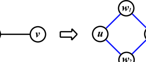
Therefore, to determine $T_{n,{\rm tot}}^{(n)}$, we need to find $\overline{T}_{n,{\rm tot}}^{(n)}$ first, which can be obtained as follows. Notice that for any given edge attaching two nodes $u$ and $v$ (see Fig. 7) in $H_{n}$, it will generate two new nodes ($w_{1}$ and $w_{2}$) in $H_{n+1}$, and the FPTs for the two new nodes are equal to each other obeying the following equation:

$$T(w_{1})=T(w_{2})=1+\frac{1}{2}\left(T(u)+T(v)\right)\,,$$ (32)

which yields to

$$T(w_{1})+T(w_{2})=2+T(u)+T(v)\,.$$ (33)

Summing Eq. (33) over all $E_{n}$ old edges belonging to $H_{n}$, we have

$$\overline{T}_{n+1,{\rm tot}}^{(n+1)} = 2\,E_{n}+\sum_{i\in\Delta_{n}}\left(k_{i}(n)\times T_{i}^{(n)}\right)$$ (34)

$$= 2\times 4^{n}+2\,\overline{T}_{n,{\rm tot}}^{(n+1)}+2^{2}\,\overline{T}_{n-1,{\rm tot}}^{(n+1)}+\ldots$$

$$+2^{n}\,\overline{T}_{1,{\rm tot}}^{(n+1)}+2^{n}\,\overline{T}_{0,{\rm tot}}^{(n+1)}\,,$$

from which we can derive the following recursive relation:

$$\overline{T}_{n+2,{\rm tot}}^{(n+2)}=16\,\overline{T}_{n+1,{\rm tot}}^{(n+1)}-2\times 4^{n+1}\,.$$ (35)

Using the initial condition $\overline{T}_{1,{\rm tot}}^{(1)}=6$, Eq. (35) is solved inductively to get

$$\overline{T}_{n,{\rm tot}}^{(n)}=\frac{4^{n}}{6}+\frac{4^{2n}}{3}\,.$$ (36)

Plugging Eq. (36) into Eq. (31), we have

$$T_{n,{\rm tot}}^{(n)}=4\,T_{n-1,{\rm tot}}^{(n-1)}+\frac{4^{n}}{6}+\frac{4^{2n}}{3}\,.$$ (37)

Combining with the initial condition $T_{1,{\rm tot}}^{(1)}=10$, one can solve Eq. (37) by induction to obtain

$$T_{n,{\rm tot}}^{(n)}=\frac{4^{n}}{18}(8\times 4^{n}+3n+10)\,.$$ (38)

Inserting Eq. (38) into Eq. (5), we obtain the rigorous solution for the MFPT for the trapping issue performed on $H_{n}$ of the $q=0$ case:

$$\langle T\rangle_{n}=\frac{1}{V_{n}-1}T_{n,{\rm tot}}^{(n)}=\frac{4^{n}}{6(2\times 4^{n}+1)}(8\times 4^{n}+3n+10)\,.$$ (39)

As in the case of $q=1$, we can recast $\langle T\rangle_{n}$ as a function of the network order:

$$\langle T\rangle_{n}=\frac{3V_{n}-4}{36(V_{n}-1)}\left[12V_{n}+\frac{3\,\ln\left(\frac{3}{2}V_{n}-2\right)}{2\,\ln 2}-6\right],$$ (40)

from which it is easy to see that for large network (i.e., $V_{n}\rightarrow\infty$), we have the following expression:

$$\langle T\rangle_{n}\approx V_{n}\,.$$ (41)

Thus, the MFPT grows linearly with increasing order of network, which is in sharp contrast to the sublinear scaling for the $q=1$ case shown above.

Figure 8: (Color online) Mean first-passage time $\langle T\rangle_{n}$ as a function of the iteration $n$ on a semilogarithmic scale for two case of $q=1$ and $q=0$. The filled symbols are the numerical results obtained by direct calculation from Eq. (5), while the empty symbols correspond to the exact values from Eqs. (25) and (39). The analytical and numerical values are consistent with each other.

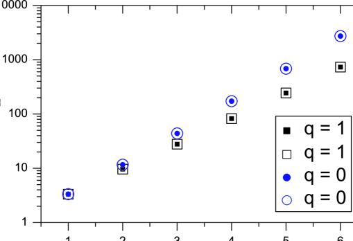
In order to confirm the analytical expressions provided by Eqs. (25) and (39), we have compared the exact solutions for the MFPT with numerical values given by Eq. (5), see Fig. 8. For all $1\leq n\leq 6$, the analytical values obtained from Eqs. (25) and (39) show complete agreement with their corresponding numerical results. This agreement is an independent test of our theoretical formulas.

III.3 Case of $0<q<1$

We have obtained the explicit expressions for MFPT of random walks with a trap on the networks for two limiting cases of $q=1$ and $q=0$, and shown that for the corresponding cases the MFPT grows sublinearly or linearly with the network order. But for the case of $0<q<1$, there are some difficulties in obtaining a closed formula for $\langle T\rangle_{n}$ as for the two special cases of $q=1$ and $q=0$, since for $q=1$ and $q=0$, the networks are deterministic and self-similar, which allows one derive the the analytic solutions for $\langle T\rangle_{n}$; while for $0<q<1$, the networks are stochastic, which makes it impossible to write a recursive relation for the evolution of the first-passage time.

Figure 9: (Color online) Mean first-passage time $\langle T\rangle_{n}$ versus the network order $V_{n}$ on a log-log scale for various $n$ and $q$. The solid lines serve as guides to the eye.

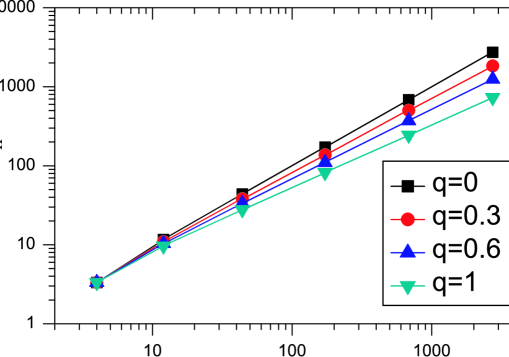
In order to obtain the dependence relation of MFPT with the network order for $0<q<1$, we have performed extensive numerical simulations for various networks with different iteration $n$ ($1\leq n\leq 6$) and $q$ between $0$ and $1$. Figure 9 illustrates the variation of MFPT with network order $V_{n}$, showing that for all $0\leq q\leq 1$, the MFPT grows as a power-law function of $V_{n}$ with the exponent $\theta(q)$ changing with $q$: When $q$ increases from 0 to 1, the exponent $\theta(q)$ decreases from 1 to $\frac{\ln 3}{\ln 4}$.

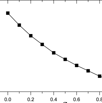
From Fig. 9 we also know that the efficiency of trapping process is closely related to parameter $q$: the larger the parameter $q$, the higher of the efficiency of the trapping problem. To show this concretely, we performed numerical calculation for network $H_{6}$ with order $2732$ for different $q$. For each fraction $q$ ($0<q<1$), all results are obtained by applying Eq. (5) to an ensemble of 100 network realizations. In Fig. 10, we plot the MFPT, $\langle T\rangle_{6}$, as a function of $q$. It is easily observed that when $q$ increases from 0 to 1, the MFPT decreases monotonically with $q$.

Figure 10: Dependence relation of MFPT on parameter $q$.

IV Conclusions

In summary, we have investigated the trapping issue on a family of scale-free networks with identical degree sequence thus the same degree distribution, which is controlled by a parameter $q$ ($0\leq q\leq 1$). We computed analytically or numerically the mean first-passage time (MFPT) for the trapping problem on the networks for various $q$. The obtained results show that for all $q$, the MFPT grows as a power-law function of network order with the exponent $\theta(q)$ dependent on $q$: when the parameter $q$ grows from 0 to 1, the exponent $\theta(q)$ decreases from 1 to $\frac{\ln 3}{\ln 4}$, which indicates that power-law degree distribution alone is not enough to characterize the trapping problem performed on scale-free networks. Therefore, when one makes general statements about the behavior of trapping issue on scale-free networks, care should be needed.

Acknowledgment

We thank Xing Li and Yichao Zhang for their assistance. This research was supported by the National Basic Research Program of China under Grant No. 2007CB310806; the National Natural Science Foundation of China under Grants No. 60704044, No. 60873040, and No. 60873070; the Shanghai Leading Academic Discipline Project No. B114, and the Program for New Century Excellent Talents in University of China (Grant No. NCET-06-0376). W L Xie also acknowledges the support provided by Hui-Chun Chin and Tsung-Dao Lee Chinese Undergraduate Research Endowment (CURE).

References

- (1) F. Spitzer, Principles of Random Walk (Van Nostrand, Princeton, New Jersey, 1964).
- (2) G. H. Weiss, Aspects and Applications of the Random Walk (North Holland, Amsterdam, 1994).
- (3) B. D. Hughes, Random Walks and Random Environments: Random Walks (Clarendon Press, Oxford, 1996), Vol. 1.
- (4) E. W. Montroll, J. Math. Phys. 10, 753 (1969).
- (5) J. J. Kozak and V. Balakrishnan, Phys. Rev. E 65, 021105 (2002).
- (6) J. J. Kozak and V. Balakrishnan, Int. J. Bifurcation Chaos Appl. Sci. Eng. 12, 2379 (2002).
- (7) E. Agliari, Phys. Rev. E 77, 011128 (2008).
- (8) R. Albert and A.-L. Barabási, Rev. Mod. Phys. 74, 47 (2002).
- (9) S.N. Dorogovtsev and J.F.F. Mendes, Adv. Phys. 51, 1079 (2002).
- (10) M. E. J. Newman, SIAM Rev. 45, 167 (2003).
- (11) A.-L. Barabási and R. Albert, Science 286, 509 (1999).
- (12) Z. Z. Zhang, Y. Qi, S. G. Zhou, W. L. Xie, and J. H. Guan, Phys. Rev. E 79, 021127 (2009).
- (13) Z. Z. Zhang, J. H. Guan, W. L. Xie, Y. Qi, and S. G. Zhou, EPL, 86, 10006 (2009).
- (14) Z. Z. Zhang, S. G. Zhou, W. L. Xie, L. C. Chen, Y. Lin, and J. H. Guan, Phys. Rev. E 79, 061113 (2009).
- (15) F. M. Atay, T. Biyikoğlu, and J. Jost, IEEE Trans. Circuits Syst., I: Fundam. Theory Appl. 53, 92 (2006).
- (16) A. Hagberg, P. J. Swart, and D. A. Schult, Phys. Rev. E 74, 056116 (2006).
- (17) V. M. Eguíluz and K. Klemm, Phys. Rev. Lett. 89, 108701 (2002).
- (18) Z. Z. Zhang, S. G. Zhou, T. Zou, and G. S. Chen, J. Stat. Mech.: Theory Exp. (2008), P09008.
- (19) Z. Z. Zhang, S.G. Zhou, T. Zou, L. C. Chen, and J. H. Guan, Phys. Rev. E 79, 031110 (2009).
- (20) H. D. Rozenfeld, S. Havlin, and D. ben-Avraham, New J. Phys. 9, 175 (2007).
- (21) C. Song, S. Havlin, H. A. Makse, Nature 433, 392 (2005).
- (22) C. Song, S. Havlin, H. A. Makse, Nature Phys. 2, 275 (2006).
- (23) A. N. Berker and S. Ostlund, J. Phys. C 12, 4961 (1979).
- (24) M. Kaufman and R.B. Griffiths, Phys. Rev. B 24, 496 (1981).
- (25) R.B. Griffiths and M. Kaufman, Phys. Rev. B 26, 5022 (1982).
- (26) M. Hinczewski and A. N. Berker, Phys. Rev. E 73, 066126 (2006).
- (27) Z. Z. Zhang, S. G. Zhou, and T. Zou, Eur. Phys. J. B 56, 259 (2007).
- (28) H. D. Rozenfeld and D. ben-Avraham, Phys. Rev. E 75, 061102 (2007).
- (29) N. Aral and A. N. Berker, Phys. Rev. B 79, 014434 (2009).
- (30) Z. Z. Zhang, S. G. Zhou, L. C. Chen, and J. H. Guan, Eur. Phys. J. B 64, 277 (2008).
- (31) S. Condamin, O. Bénichou, V. Tejedor, R. Voituriez, and J. Klafter, Nature (London) 450, 77 (2007).
- (32) S. Redner, A Guide to First-Passage Processes (Cambridge University Press, Cambridge, 2001).
- (33) A. Bar-Haim and J. Klafter, J. Chem. Phys. 109, 5187 (1998).
- (34) J. G. Kemeny and J. L. Snell, Finite Markov Chains (Springer, New York, 1976).
- (35) F. R. K. Chung. Spectral Graph Theory, Am. Math. Soc., Providence, RI, 1997).
- (36) S. Havlin and D. ben-Avraham, Adv. Phys. 36, 695 (1987).
- (37) B. Kahng and D. Redner, J. Phys. A: Math. Gen. 22, 887 (1989).
- (38) E. M. Bollt, D. ben-Avraham, New J. Phys. 7, 26 (2005).